A Machine Learning Approach to Extract Rock Mass Discontinuity Orientation and Spacing, from Laser Scanner Point Clouds

Abstract

This study wants to give a contribution to the semi-automatic evaluation of rock mass discontinuities, orientation and spacing, as important parameters used in Engineering. In complex and inaccessible study areas, a traditional geological survey is hard to conduct, therefore, remote sensing techniques have proven to be a very useful tool for discontinuity analysis. However, critical expert judgment is necessary to make reliable analyses. For this reason, the open-source Python tool named DCS (Discontinuities Classification and Spacing) was developed to manage point cloud data. The tool is written in Python and is based on semi-supervised clustering. By this approach the users can: (a) estimate the number of discontinuity sets (here referred to as “clusters”) using the Error Sum of Squares (SSE) method and the K-means algorithm; (b) evaluate step by step the quality of the classification visualizing the stereonet and the scatterplot of dip vs. dip direction from the clustering; (c) supervise the clustering procedure through a manual initialization of centroids; (d) calculate the normal spacing. In contrast to other algorithms available in the literature, the DCS method does not require complex parameters as inputs for the classification and permits the users to supervise the procedure at each step. The DCS approach was tested on the steep coastal cliff of Ancona town (Italy), called the Cardeto–Passetto cliff, which is characterized by a complex fracturing and is largely affected by rockfall phenomena. The results of discontinuity orientation were validated with the field survey and compared with the ones of the FACETS plug-in of CloudCompare. In addition, the algorithm was tested and validated on regular surfaces of an anthropic wall located at the bottom of the cliff. Eventually, a kinematic analysis of rock slope stability was performed, discussing the advantages and limitations of the methods considered and making fundamental considerations on their use.

1. Introduction

In rock mass characterization, a good understanding of the discontinuity network within a rock mass, such as joints and bedding planes, is essential to control failure mechanisms. To this aim, the description of discontinuity properties such as spacing, persistence, roughness, weathering, infilling, etc. is important for engineering design [1,2] and can be performed in the field using standardized methods, such as scanline surveys [3,4] or more recently, the use of remote sensing techniques such as Laser Scanning coupled with a semi-automated discontinuity analysis [5,6,7]. Although the measure of discontinuity orientation based on the geological compass is the most accepted, large errors may be introduced due to sampling difficulties caused by the inaccessibility of the site, representativeness of the data, and considerable safety risks due to unstable slopes [8]. The data collection based on point cloud analysis has both advantages and disadvantages in rock slope engineering [6,7]. The main advantage is that the laser scanning surveys can be carried out rapidly and at a distance that allows for safe surveying and permits obtaining a rapid and consistent discontinuity properties database of inaccessible spots [7]. However, limitations and biases related to the surface coverage and orientation of the laser beam must be considered [9,10,11].

A discrete number of algorithms are available in the literature for discontinuity extraction, such as Split-FX [7], COLTOP [12] and PlaneDetect [13], and from the 3D point cloud, e.g., FACETS [14], RANSAC [15] SMRTool [16], in addition to several others working on point clouds for rock mass characterization [17,18,19,20,21,22,23,24,25,26,27,28,29,30]. Within these approaches, it is possible to discriminate between the ones working with raw point clouds and the ones in which the surfaces are derived. Creating planar surfaces from point clouds leads, at first, to a simplification and often to an erroneous interpretation of the original data. Moreover, the quality of the results obtained with this method is strictly related to the parameters used for the classification and to the criteria used to group the acquired points. Instead, working with raw point clouds has the advantage of maintaining the original resolution without any resample and avoiding polygonal surfaces derived from the triangular interpolation [22]. However, one disadvantage is that of having longer computation time, especially when processing very large areas.

Our approach works exclusively on the point cloud, operating a classification based on the Error Sum of Squares (SSE) method and K-means algorithm, aimed to derive the proper number of discontinuity sets to be used (hereinafter referred to as “clusters”). The code is available at: https://github.com/vrai-group/geospacing, (accessed on 1 May 2022). The end-users can estimate the number of clusters with automatic or manual initialization of centroids. End users can also manually specify the exact number of clusters by also providing initial values for centroids. Then, it is possible to evaluate step by step the results of the cluster classification by visualizing the stereographic projections.

After discontinuity identification and classification, it is possible to analyze discontinuity spacing. To this aim, a discrete number of algorithms and approaches already exist: (a) the ones working similarly to the fieldwork approach using profile sections or virtual scanlines [31,32] or analyzing two-dimensional fracture trace information [8]; (b) the ones analyzing spacing using 3D spatial relations [22,31,32,33]. Our approach belongs to the method of analyzing spacing using 3D spatial relations. The normal set spacing is calculated as the average of normal distances between individual discontinuities within a discontinuity set, as reported by [34]. Finally, the results obtained were compared with those derived from the traditional geomechanical survey to make considerations on the kinematic stability analysis carried out according to Markland’s test [35]. The main aim of this paper is to propose a straightforward semi-supervised procedure for calculating discontinuity mean set orientation and spacing, starting from the 3D point cloud, and to discuss the advantages and disadvantages of this method, comparing it with the field data and with the FACETS algorithm.

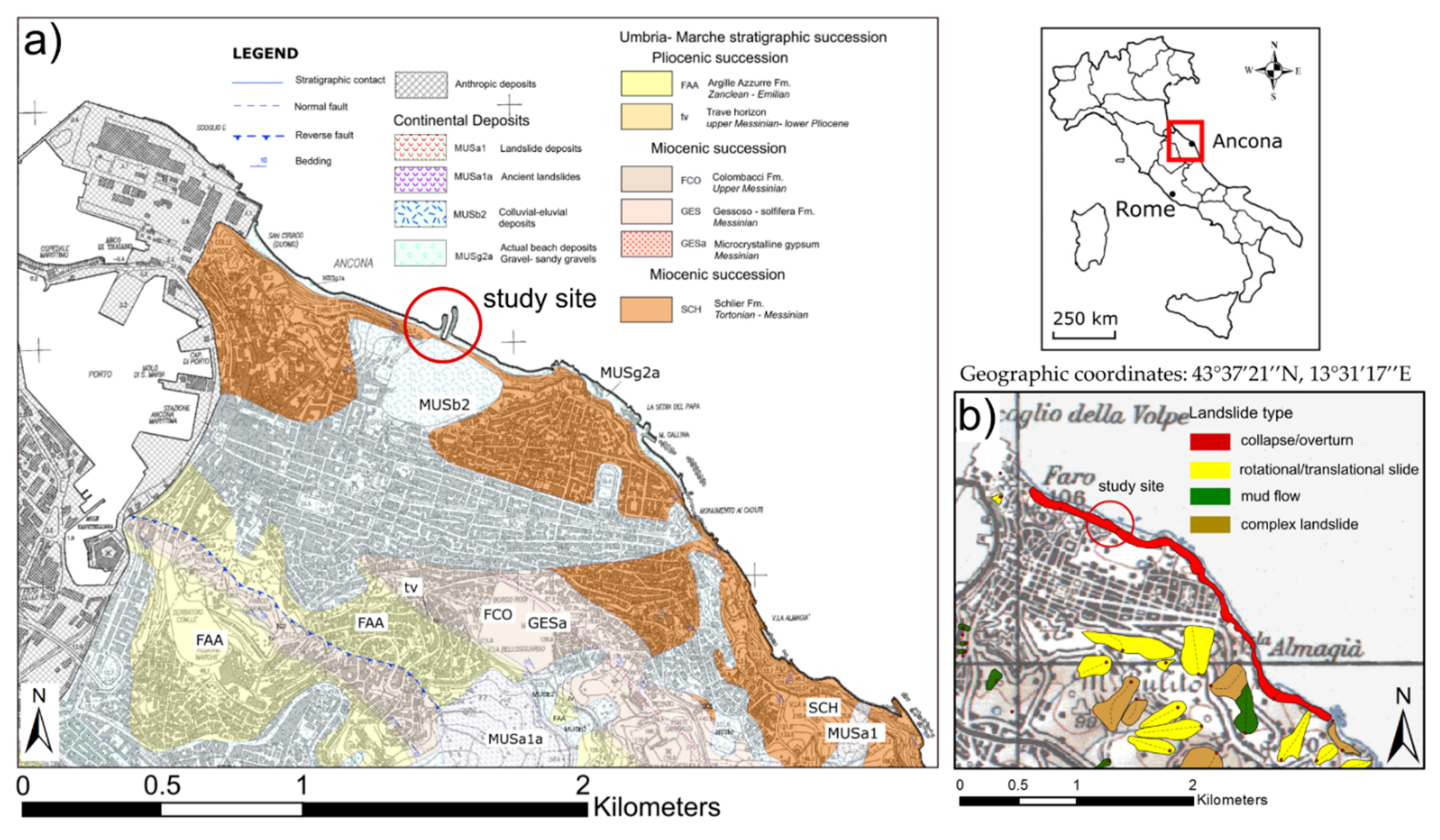
2. Geological Framework of the Area

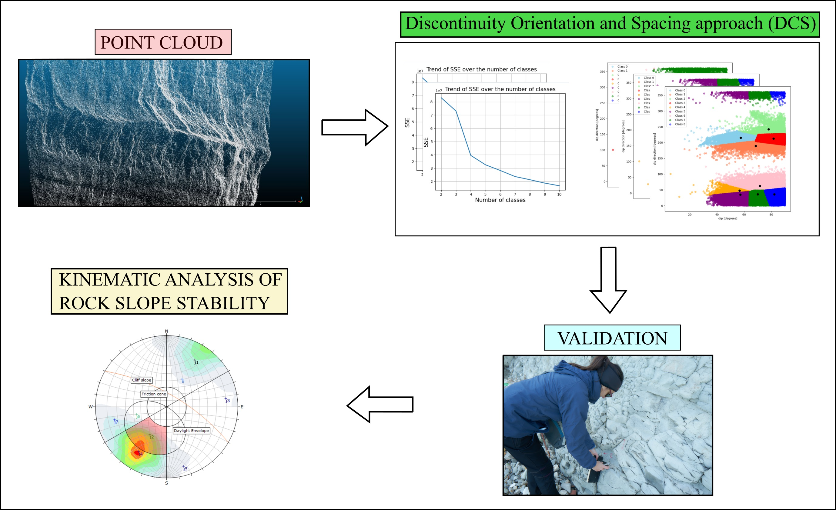
The coastline of Ancona town (Marche Region, Central Italy) is characterized by steep active cliffs with an average height of over 60–80 m, whose morphology is strictly related to the lithological and structural characteristics of the incompetent Neogene marly formations of the Umbria–Marche stratigraphic sequence. From a geological point of view, the early–mid-Miocene represents the beginning of the Alpine–Himalayan orogenesis. Synorogenic siliciclastic foredeep oriented NW-SE were filled by marly flysch and thick sandy deposits, as the orogenic front advanced eastward, accompanying extensive folding and thrusting [36]. The coastal cliffs of the Ancona and Mt. Conero riviera are the results of the easternmost part of the Umbria–Marche basin, where pelagic limestones and marls continued to sediment until the Late Miocene [37,38]. During the late Burdigalian–early Messinian time [39,40], an important extensional tectonic event affected the Apennines. During this event, which was probably connected with the flexure of the Adriatic foreland lithosphere, pre-thrusting NW-SE striking normal faults developed, and they were reactivated as back thrust faults during the compression phase, in which the Mt. Conero anticline developed. The high geo-structural complexity of the area, coupled with the steep morphology of the cliffs directly overhanging the sea and their poor geomechanical characteristics make the whole coastal area (9 km long) between the promontory of the Mt. Conero and the port of Ancona an active high coast [41,42]. As reported by several studies [42,43,44,45,46,47,48,49], all the coastal area is characterized by rock falls, collapses–overturn, detrital roto-translational slumps, and rock translational slumps.

In detail, the Cardeto–Passetto sea cliff is characterized by 60–70 m high outcrops of the marly–clayey lithologies of the Schlier Formation (Lower Messinian–Burdigalian) (Figure 1) made up of alternances of marlstones and calcareous marlstones with varying percentages (35–80%). In the geological formation, the calcium carbonate content decreases from the bottom to the top. The choice of this area was driven by several factors: (a) the need to improve the know-how of the area, especially from a stability standpoint; (b) the presence of both planar and rugged surfaces; (c) the irregular block shapes within the rock mass. As reported by previous studies [50,51], rock slope instabilities mostly occur in the calcareous–marly portion of the Schlier geological formation, while mudflows are frequent where the rock matrix has a predominantly clayey–marly composition. The thick debris covering the outcrops at the bottom of the cliff (Figure 1) is the main cause of the inaccessibility of the site for a traditional geological survey.

3. Methodology

3.1. Traditional Geomechanical Survey

To validate the machine learning approach proposed in this paper, two traditional geomechanical surveys were conducted at the base of the sea cliff where only rock outcrops are present (light blue stars in Figure 2), by performing 10–12 m one-dimensional (1D) scan lines oriented perpendicular to each other. Orthogonal scanlines allow for measuring all the sets of discontinuities present more accurately. The term “discontinuity”, as reported by [53], refers to all the geological features of the rock mass that share the common characteristics of low shear strength, negligible tensile strength and high fluid conductivity compared to the surrounded rock materials. The term “discontinuity” includes bedding planes, faults, fissures, fractures, joints, veins, stylolites, etc., avoiding any inferences concerning their geological origins. All the discontinuity measurements were corrected through the Terzaghi approach [54] and grouped into discontinuity sets by observing pole concentration using a contour plot. The stereographic projections were made using the Rocscience Dips software [55]. Is important to note that, although the scanline survey was carried out in different locations than the laser scanner survey, at this scale of observation, the orientation of the discontinuity surfaces is considered constant from a geological point of view. As far as the spacing is concerned, it can undergo variations linked to the hardness variation of the lithologies which constitute the Schlier geological formation. However, by examining a large area with the laser scanner, the value of the spacing is averaged and is therefore comparable with that derived from the classical geomechanical survey.

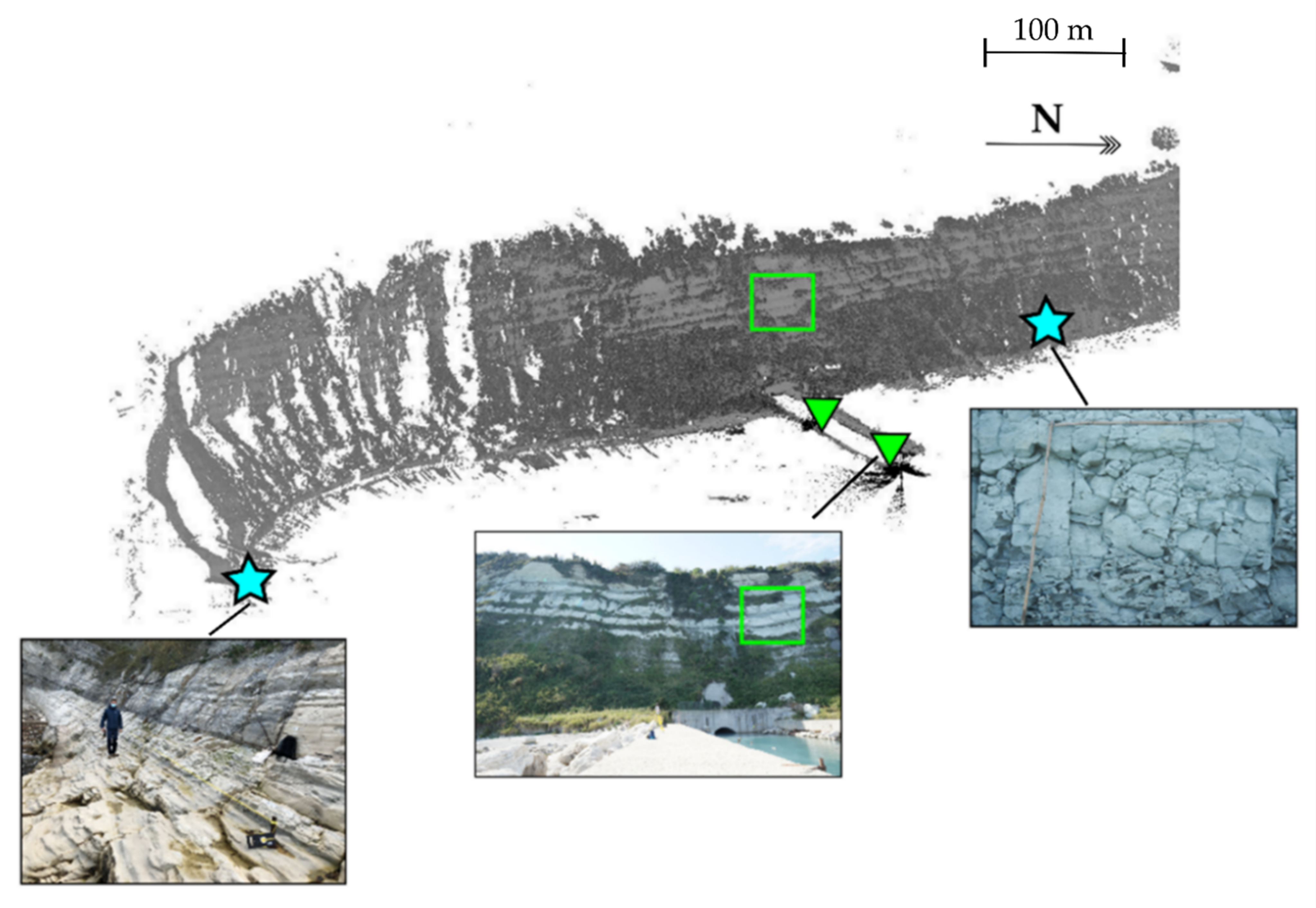
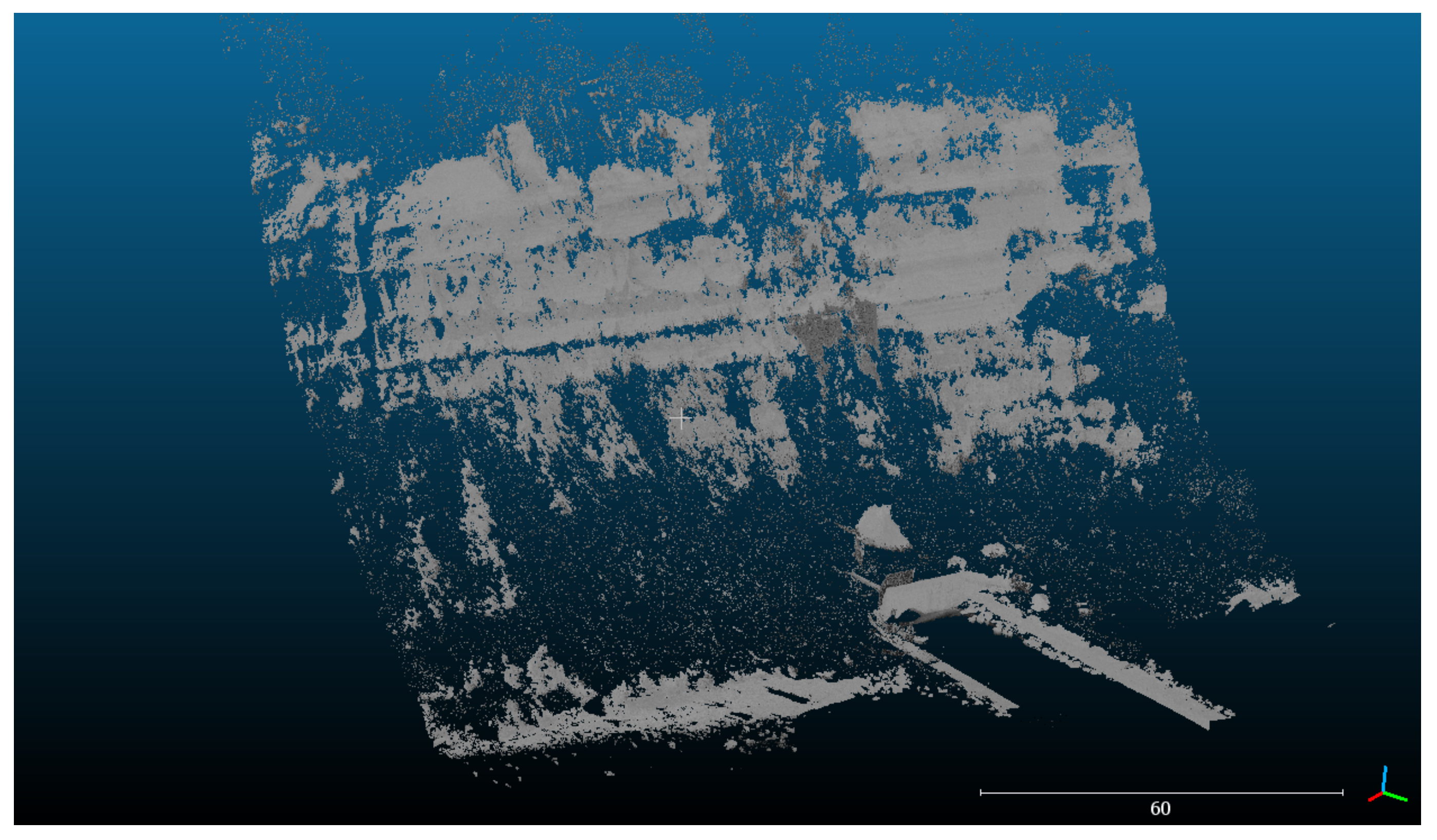
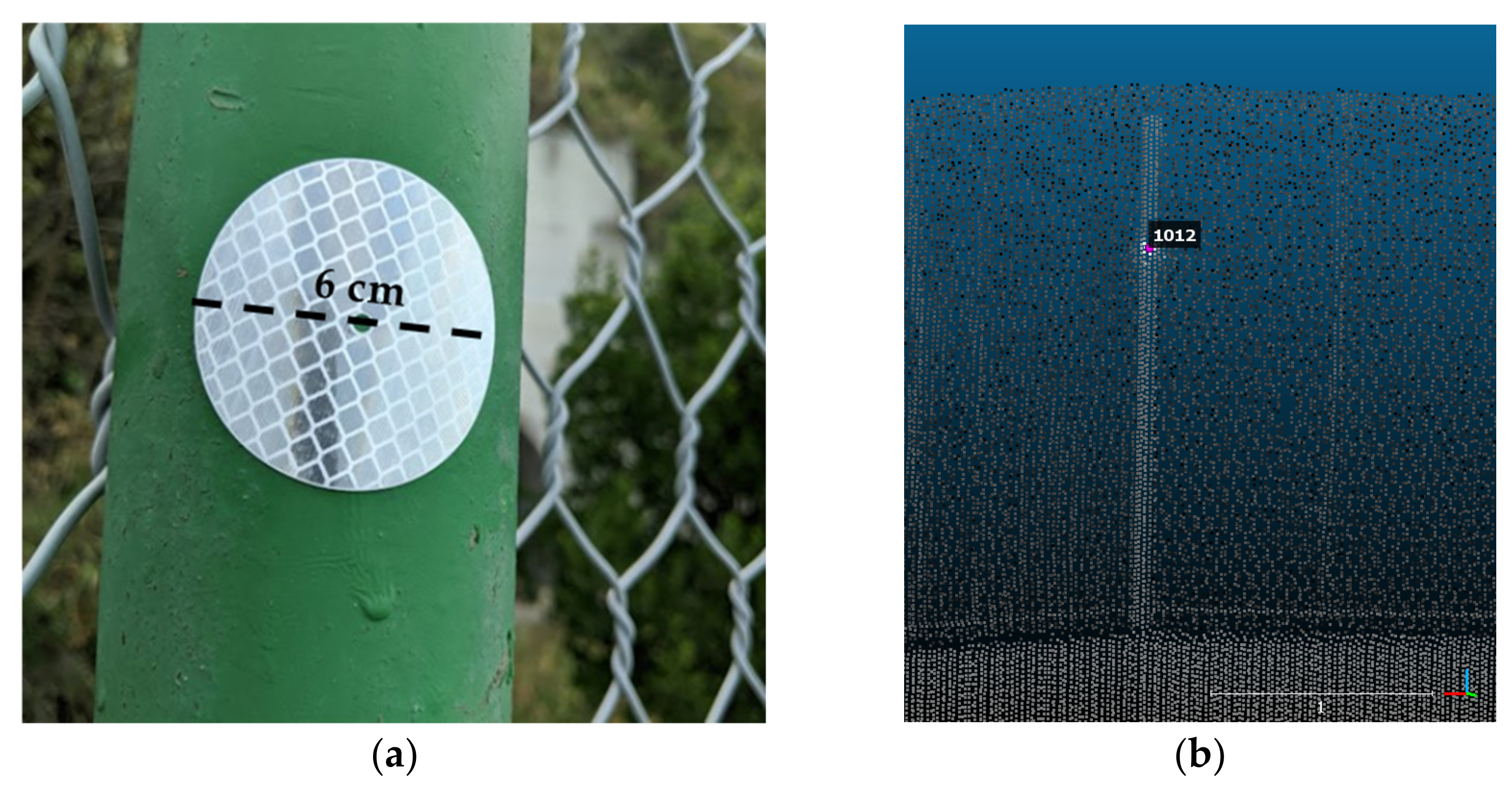
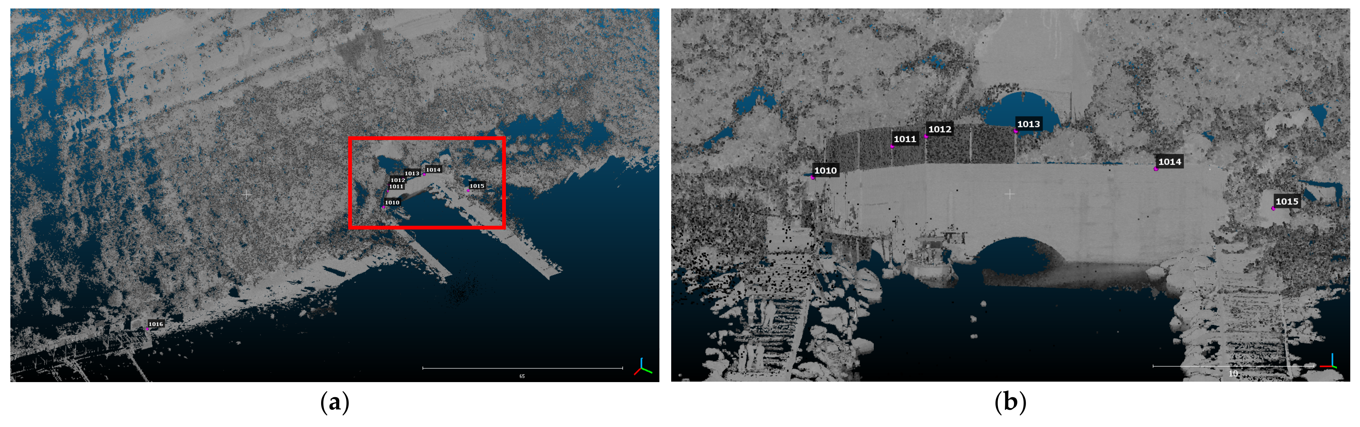
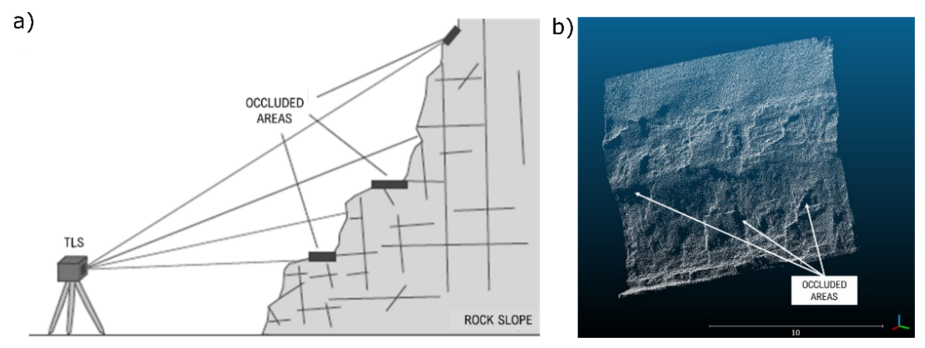
3.2. Terrestrial Laser Scanner Data Acquisition

In addition to the traditional geological fieldwork, a geomatic survey was carried out using a Terrestrial Laser Scanner (TLS) to obtain a three-dimensional (3D) model of the rock face. The TLS was positioned on a pier in front of the rock face of interest (green triangles in Figure 2), at a distance of approximately 100 m, to have a greater acquisition and reduce orientation bias in both the horizontal and vertical planes. The TLS RIEGL VZ-400i was able to acquire a dense, georeferenced point cloud consisting of 30 million points, each with the following information: position (X, Y, Z), color (RGB), and reflectance (i). During the scanning setup phase, the photography data were also set regarding exposure time and aperture to connect the images to the point cloud.

The images were appropriately calibrated according to the light conditions and the proximity of the object of investigation. In the end, a detailed scan of the targets was performed, which allowed the scanner to locate and record 7 installed reflectors (Figure 3). The choice of the instrument had good technical characteristics that largely satisfy the detail requirements such as: (a) the possibility of selecting the area to be surveyed by manually identifying it through the instrument’s control monitor; (b) the ability to reduce the shadow zones due to vegetation; (c) the 800 m operating range (100kHz laser pulse); (d) the high acquisition speed of 240 lines/s (vertical scan) [56]; (e) the high metric performance, which is confirmed by the high level of accuracy achieved in georeferencing the targets through the topographic survey carried out (Figure 4,

Table 1. TLS point cloud alignment information.

Final RMS [m]	0.0164765
Transformation matrix	0.999	0.043	0.000	−61.794
	−0.043	0.999	0.000	113.865
	−0.000	−0.000	1.000	47.718
	0.000	0.000	0.000	1.000
Scale [m]	0.999695

).

To achieve greater completeness in the definition of the surfaces in the 3D model of the cliff, it would have been necessary to perform other scans from different viewpoints. Unfortunately, there are no other suitable points to satisfy this need because, in the area, only one pier is available as a suitable place to place the laser scanner. This was the main cause of occlusion. Based on this, some portions of the rock wall are oriented in the opposite direction from that of the laser beam, which causes blind zones in the point cloud, which can partially affect the results of the discontinuity characterization [57]. The tested area has an extension of 25 m × 13 m. The data acquired via TLS were then processed using Cloud Compare software. The same software allows for a cleaning operation that removes the vegetation. Thanks to the CANUPO plug-in, a supervised classification is possible to discriminate between the vegetation and the rock faces (Figure 5c). The classifier was obtained automatically with a linear SVM (Support Vector Machine) [58]. Through a statistical representation, based on the number of scales used to train the classifier, a plane of maximal separability (boundary) divides the points into the two classification components. The more scales you set, the more discriminative the result might be, but also the longer the computations. The overall balanced accuracy is 97%. Through the stratigram obtained, it is possible to identify the points that are close to the threshold values or that have not been well classified in the two categories (representing the residual component) (Figure 6). The latter will partly influence the subsequent procedure of discontinuity classification, but due to the results obtained through the traditional geomechanical survey, these will be easily identified and discarded. Figure 7 shows the result of a filtered point cloud of a rock surface after the removal of vegetation coverage.

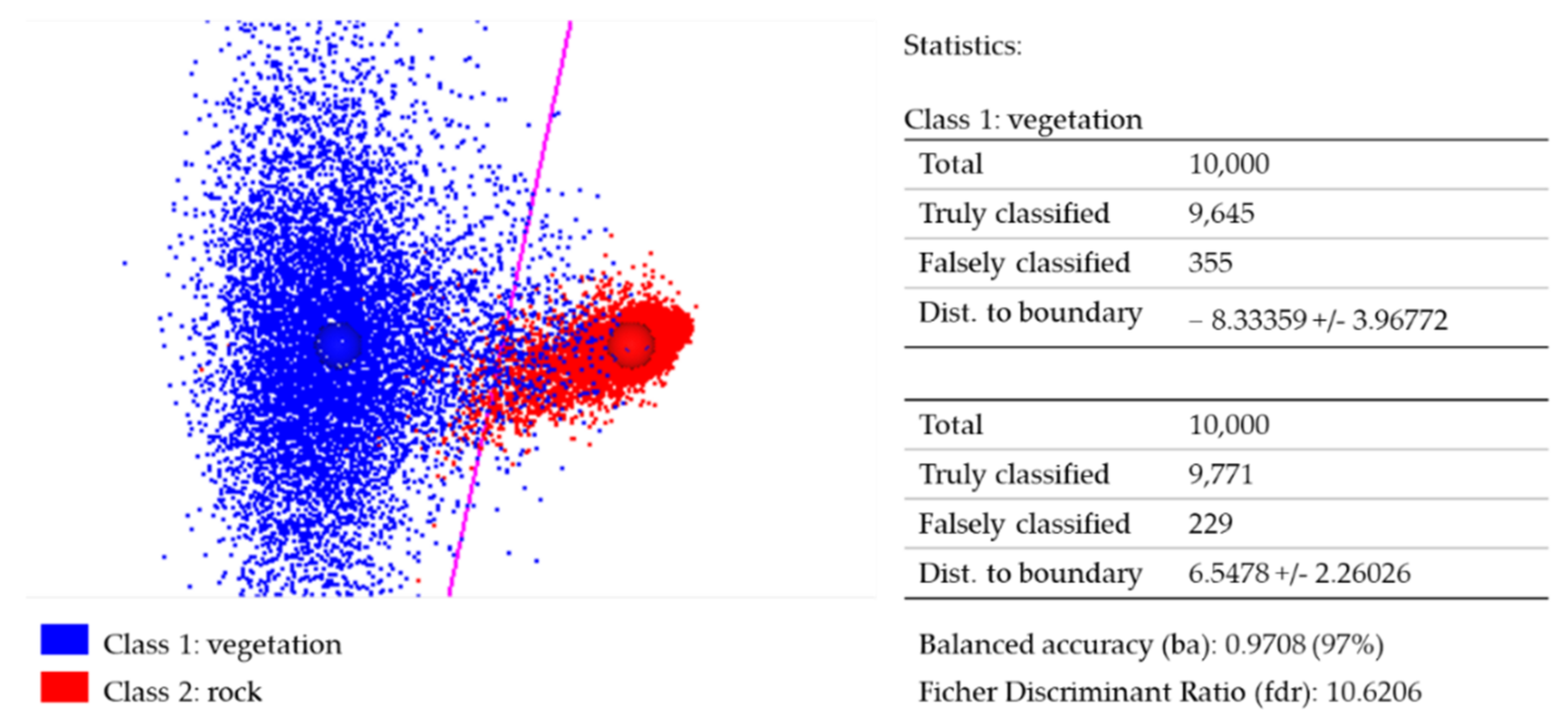
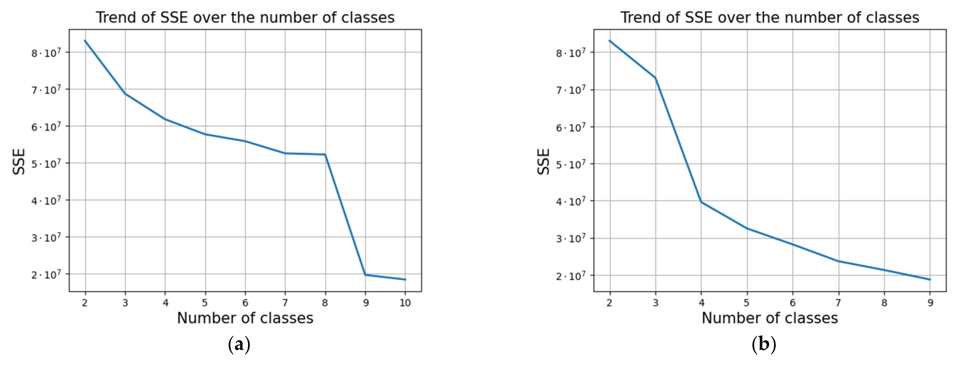
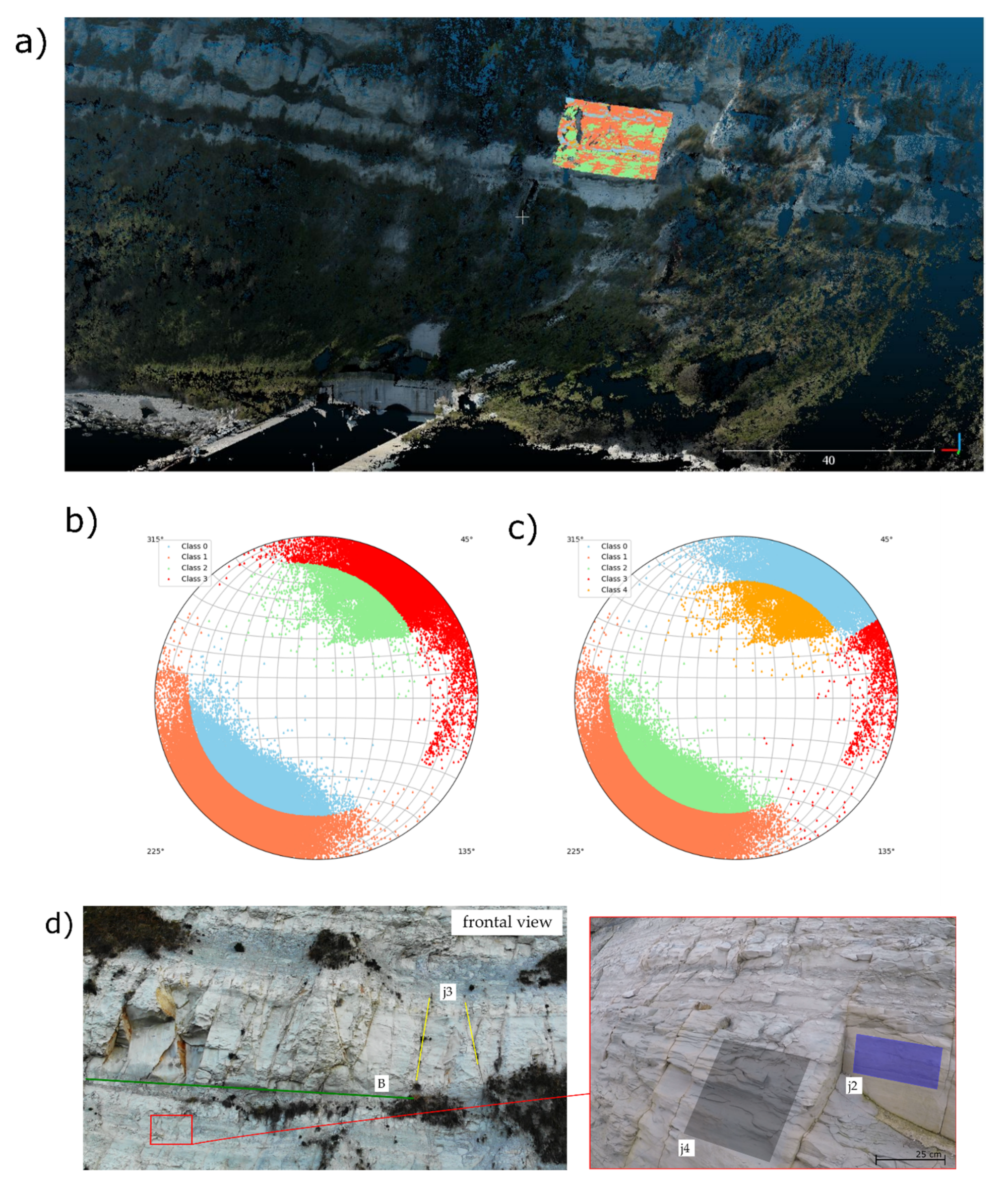
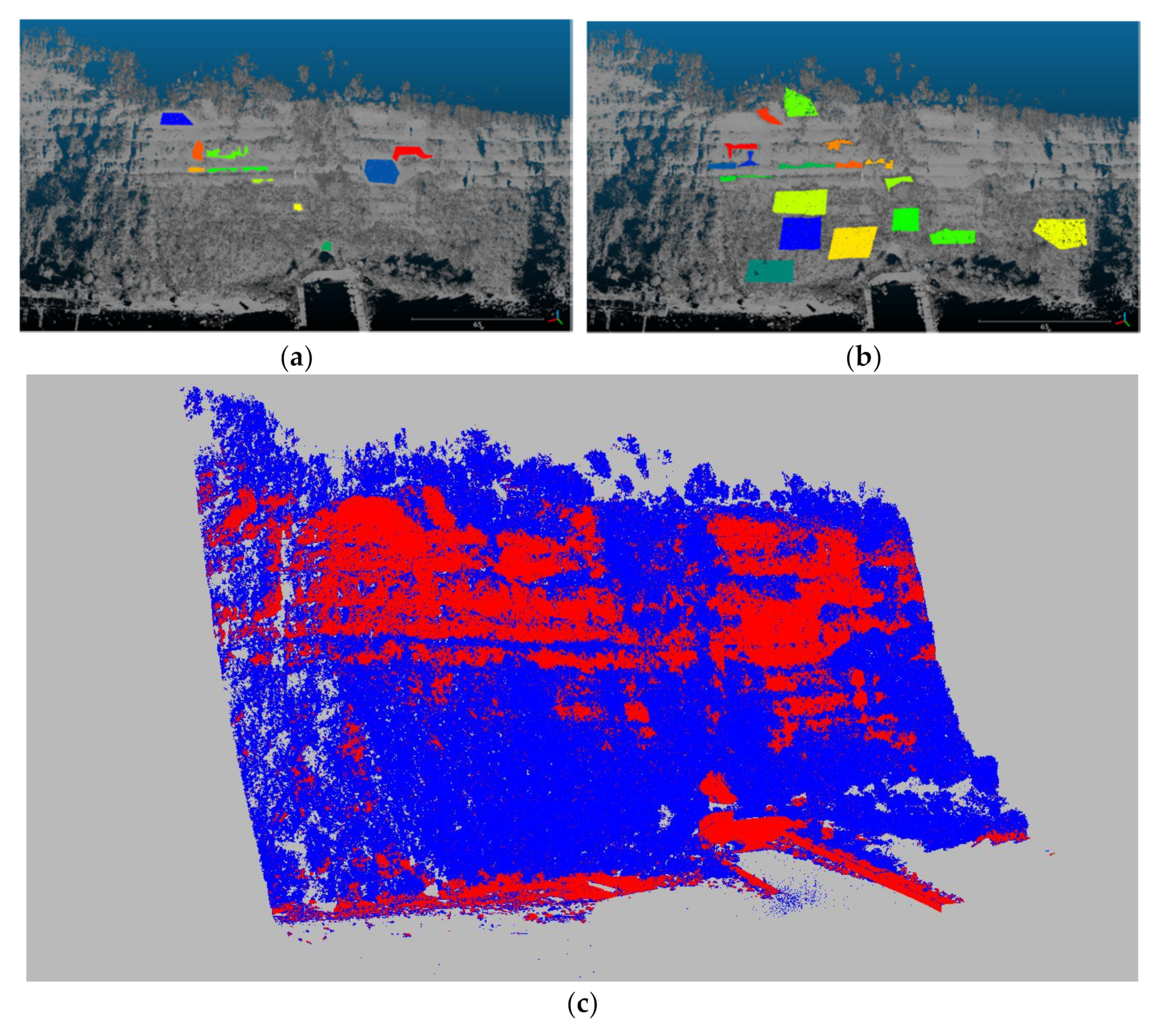
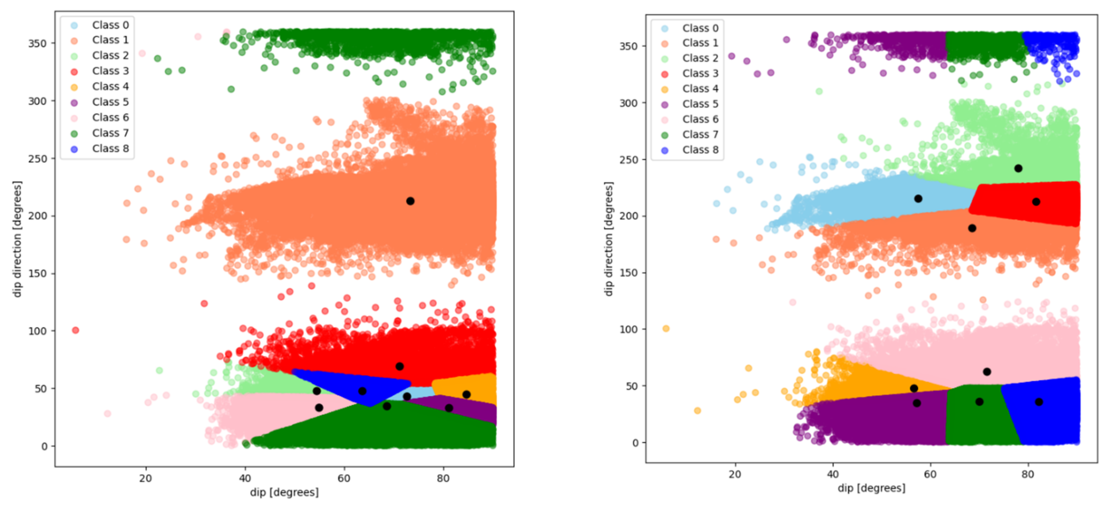
3.3. Extraction of Discontinuity Orientation and Their Classification in Clusters

The first stage of our processing pipeline is represented by the calculation of dip and dip direction starting from the data set. The point cloud was pre-processed using the Cloud Compare software to generate the normal vectors for each point, then, the normal vectors are used to calculate the dip and dip direction.

The sets of dip and dip direction are used to perform clustering using the K-means algorithm, aimed at group points with similar dip and dip directions. We used a custom distance to cluster data instead of a classical L2-norm. When we evaluate the distance between two angles, ${\theta }_1$ and ${\theta }_2$, it is necessary to consider the following expression:

$$d\left({\theta }_1,{\theta }_2\right)=\min \left(2\pi -\left|{\theta }_1-{\theta }_2\right|,\left|{\theta }_1-{\theta }_2\right|\right)$$

Then, the distances between pairs of dip and dip direction values were evaluated using the following formula:

$$distf\left({\alpha }_1,{\alpha }_2,{\beta }_1,{\beta }_2\right)=\sqrt{dist{\left({\alpha }_1,{\alpha }_2\right)}^2+dist{\left({\beta }_1,{\beta }_2\right)}^2}$$

where α and β are dip and dip direction values related to different points. This kind of formulation enables the clustering of angles that are close, avoiding issues of simple L2-norm that could lead to wrong results (e.g., the classical distance between two values as 2π – ε and ε leads to 2π – 2ε; the real distance is instead 2ε.

The number of clusters was estimated using the Error Sum of Squares (SSE) method that evaluates the sum of the squared distance between the centroid and each member of the cluster [45]. In this way, it is possible to derive the proper number of clusters for the data under test. A key point of our procedure regards the possibility for the users to supervise the procedure once the algorithm has classified the point cloud. In such a case, semi-supervised learning is built on the output of the unsupervised learning process. Especially when dealing with a high-resolution point cloud, the density of points with a certain value of dip and dip direction can influence the clustering result. In this way, areas of low density can be classified by the algorithm as part of another cluster, although the dip and dip direction values are considerably different. This aspect can be very important from a slope stability point of view, since less common surfaces may produce failures. On this premise, starting from values collected in situ regarding dip and dip direction (values derived from direct measurements or direct observation), it is possible to replace random centroid initialization with a manual ones.

The results of the DCS approach were compared to the FACETS/Fracture detection plug-in of Cloud Compare [14]. It is important to remark that, in contrast to the approach proposed in this study, which is based on a classification of the point cloud, the kd-tree algorithm of FACETS starts from the normal vector of the point and then merges the adjacent cells into facets [14]. The facets must share a common dip and dip direction specified by the max angle parameter and if their distance along their common normal vector is smaller than the max distance that has been set. After that, facets are aggregated into polygons, progressively, according to a planarity threshold. Taking into account the residual noise left by the vegetation removal process, families with a number of facets less than 3% over the total were not considered.

3.4. Spacing Calculation

The spacing of discontinuities is defined as the distance measured perpendicularly between two discontinuity planes belonging to the same set [53], and it is calculated by averaging the modal spacing of values measured for discontinuities of the same set. The spacing is an important parameter in rock mass characterization because it determines the block size, which is relevant to the mechanical behavior of rock masses. In the field, spacing is determined from the scanline survey, choosing a length of the tape that is sufficiently representative of the frequency of discontinuities (at least three meters). As reported by De Vallejo [53], the general rule is that the measurement length should be ten times higher than spacing.

However, in the point cloud, once the clustering is performed it is possible to calculate the normal spacing for each cluster. In particular, the spacing requires a point decimation that is performed by evaluating the distance among points using the mean normal vector for that class. The distance is evaluated using points and a normal vector (mean normal one for the chosen class) according to the following formula:

$$d\left(N,P_2,P_1\right)=\frac{\overrightarrow{N} ·\left(\overrightarrow{P_2}-\overrightarrow{P_1}\right)}{\left|\overrightarrow{N}\right|}$$

where N is the normal, $P_2$ is a given (3d) point and $P_1$ is a reference point.

Points that are inside a given threshold T are merged and this enormously reduces the amount of data to process. The threshold can be chosen by the users. Starting from the decimated points, it is possible to calculate the spacing. For each class, we apply the following procedure. We select a point $P$ that we use as a reference; then for each pair $\left(P,P_j\right)$ with $j=1,\dots ,N_i$ with $N_i$ equals the number of a point belonging to a class $i$, we calculate the distances using the normal vector equation considering N as the average of all normal vectors of points that belongs to the considered class. The distances are then sorted, and a gradient operator (first derivative) is then applied.

We applied a filter to reduce the noise on the gradient values; the filter excludes points that are too close. This situation, if not managed, could lead to a wrong evaluation of spacing. Values are then processed and it is possible to derive basic statistics as the minimum, average, and standard deviations that could be correlated with data collected in situ.

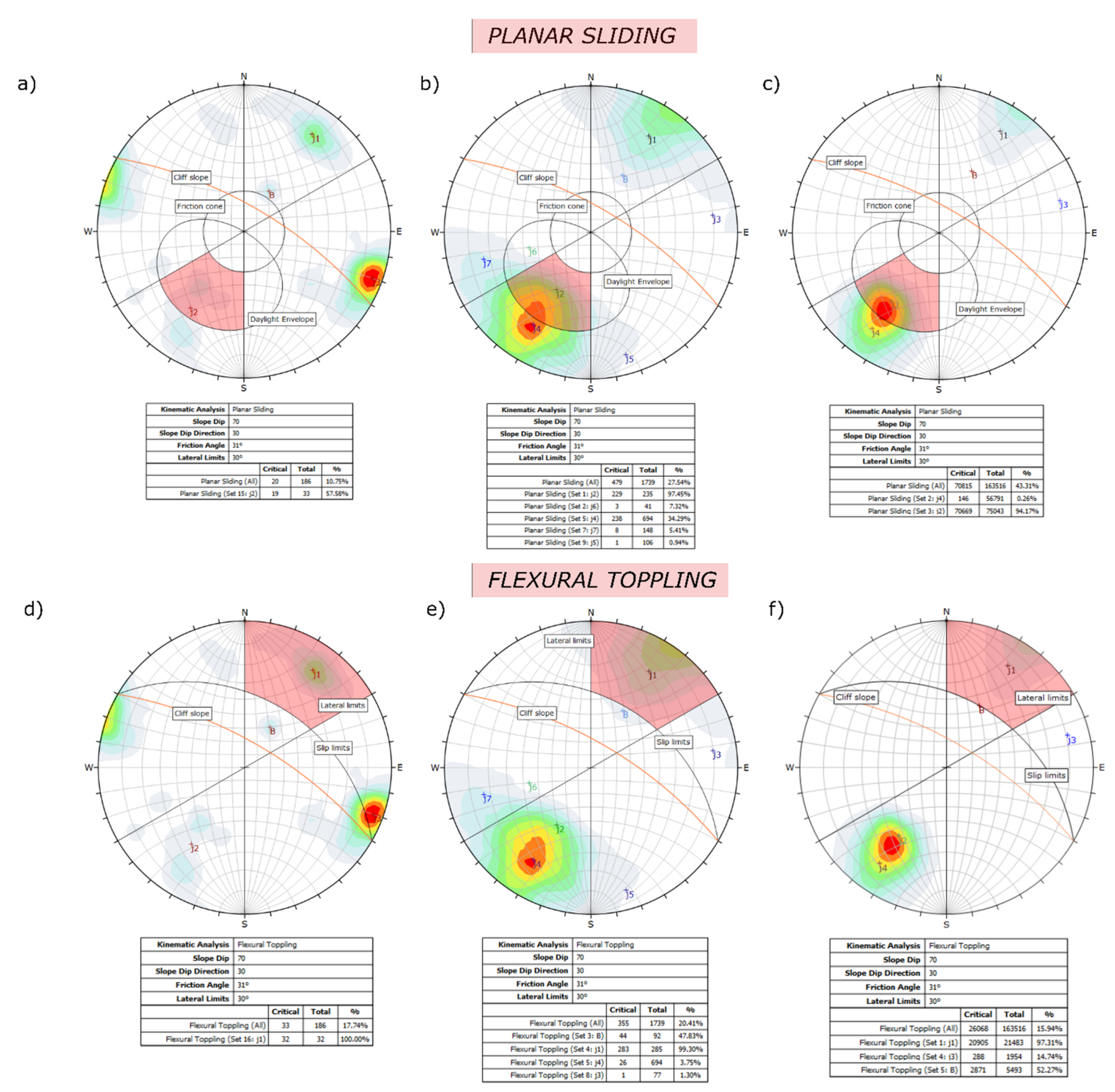
3.5. Kinematic Analysis of Slope Failure

When dealing with geomechanical data of rock slopes, one of the most important applications is kinematic analysis. The kinematic analysis is the first step in rock stability assessment and involves the interpretation of spatial relations of the geological discontinuities concerning the rock slope to determine the potential for the various kinematics, such as planar sliding, and wedge or toppling sliding [57,59]. For the Cardeto–Passetto cliff, a kinematic analysis of planar failure and toppling failure was conducted using the Rocscience DIPS v. 7.0 program [55], with the aim to identify the main slope kinematics of this area and to compare the results with the TLS survey. The analysis, called Markland’s test [35], follows the procedure described in [55], plotting and analyzing the orientation pattern on stereonet, and calculating the probability of any failure mode considering the relationship between the geometry of the slope and the friction angle. Discontinuity data were plotted on equal-area projections (Lambert–Schmidt equatorial nets).

In rock mechanics, few types of friction angles or discontinuities such as peak, residual, and basic friction angles of discontinuities are considered. They can be estimated from the triaxial test, uniaxial compressive test, direct shear test and tilt testing. In this framework, the peak friction angle acting on sliding planes is a common input in estimating the mode of failure, and it is used to represent the friction cone trace [60]. In this study, the friction circle was drawn assuming a value of 31°, based on the laboratory geotechnical test results obtained by [47], which correspond to the peak friction angle of the Schlier geological formation sampled in the same area. Fracture poles falling both outside the friction circle and inside the daylight envelope are susceptible to planar sliding. Flexural toppling failure occurs where the discontinuities dip steeply away from the slope, striking parallel or sub-parallel to it. The stability of the blocks is strictly conditioned by the shear strength of the discontinuity. Based on [61], the key elements of flexural toppling kinematical analysis are the slope plane, the slip limit plane (based on the slope angle and the friction angle), and the lateral limits.

4. Results

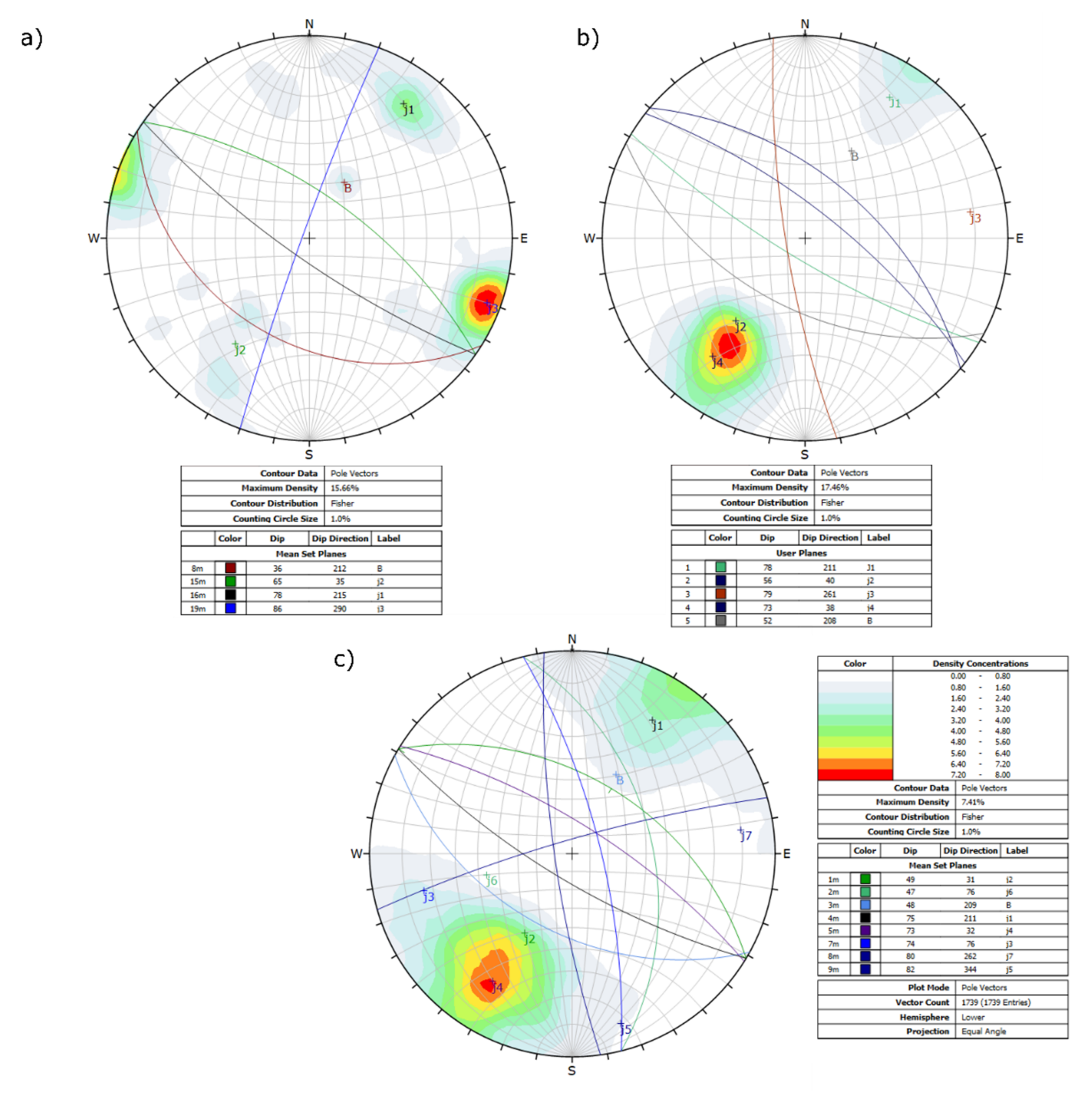
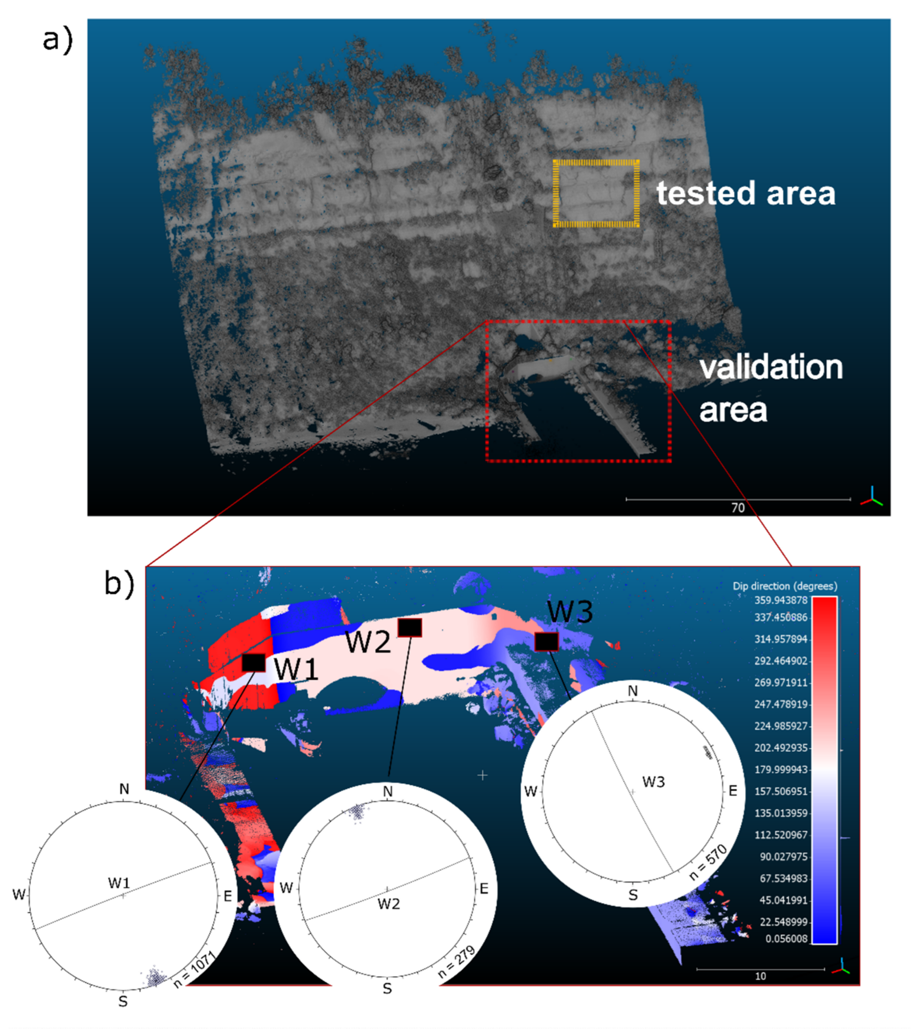
4.1. Identification of Discontinuity Sets in the Tested Area

The results of the DCS approach were compared with the field measurements and the results of the FACETS algorithm. In the first step of the DCS approach, the optimal number of clusters was defined using the SSE method (Figure 8). Using automatic initialization of centroids, the algorithm could generate a set of clusters that do not correspond with the on-site measurements (see Figure A1 left) leading to over-clustered areas and also a wrong number of classes. Using manual initialization user controls, the starting values and the SSE method puts in evidence that four classes are representative of our study area (see Figure A1 right). In order to supervise this step of discontinuity classification is important to consider the expert fieldwork observations, which should guide the appropriate evaluation of the number of clusters. After the evaluation of the criterion, it is possible to select the number of classes that will be used to perform the clustering using the K-means algorithm. In our case, based on what was observed in the field, the more appropriate number of clusters (including the bedding) is four, matching the SSE method with the manual initialization of centroids.

The K-means algorithm considers a set of features in the dip and dip directions. In Figure 9a, an overview of the photogrammetric images is reported, together with the classified point cloud. The colors of Figure 9a refer to the stereonet in Figure 9c. Figure 9b shows the stereonet of the results of K-means applied to our data set considering K = 4.

Starting from the results of the unsupervised clustering (Figure 9b) with K = 4, it is possible to re-classify cluster 3 (red poles) into two different clusters, respectively, the light blue and red poles of Figure 9c. This can be performed by running the clustering on a specific cluster again and selecting K = 2. The accuracy of the orientation estimation by DCS was compared with that of the FACETS plug-in of Cloud Compare and with the field results (

Table 2. Dip direction and dip angles of the poles of each identified discontinuity set. The relating number of points over the total number of points is reported in percentage.

Cluster ID	Field Survey Orientation (F)	DCS Algorithm		FACETS Orientation
	DA/DD [°]	DA/DD [°]	Δmc	(DA/DD) [°]	Δmc	ΔDSC-F
j1	76/203	78/211	2/−8	75/211	1/−8	−3/0
j2	66/36	73/38	−7/2	73/32	−7/4	0/6
j3	80/290	79/261	1/29	79/262	1/28	0/−1
j4	n.d./n.d.	56/40	n.d./n.d.	49/31	n.d./n.d.	7/9
Bedding (B)	36/212	52/208	n.d./n.d.	48/209	−12/3	4/−1
j5	n.d./n.d.	n.d./n.d.	n.d./n.d.	73/344	n.d./n.d.	n.d./n.d.
j6	n.d./n.d.	n.d./n.d.	n.d./n.d.	47/76	n.d./n.d.	n.d./n.d.
j7	n.d./n.d.	n.d./n.d.	n.d./n.d.	74/76	n.d./n.d.	n.d./n.d.
RMSE	n.a	9.01/15.2		7.0/14.8		19.8/14.7

Where n.a. = not available; n.d. = not detected; DA = dip angle; DD = dip direction; Δmc = difference between measured and calculated dip and dip direction. ΔDCS-F = difference between dip/dip direction calculated by DCS and FACETS.

). Pictures showing the discontinuity sets derived by the DCS approach are reported in Figure 9d. In addition, the orientation of all the sampled point normal vectors are plotted on the stereographic projection (lower hemisphere), together with mean set planes and a contour plot, the fieldwork results (Figure 10a), the DCS results (Figure 10b) and FACETS results (Figure 10c). With regards to the Cloud Compare FACETS plug-in, a combination of parameters such as maximum angle, maximum relative distance, minimum points per facet and maximum edge length are required. The parameter setting is not straightforward and thus, many iterations were made in order to test their influence on the classification results (not shown). With FACETS, twelve clusters were identified, a higher number with respect to the DCS approach and the field results. However, after discarding the clusters with a number of polygons less than 2% over the total, eight clusters were considered for analysis. Comparing the RMSE values in Table 2, the DCS method provides similar results with respect to FACETS, which displays similar RMSE values. Considering the Root Mean Squared Error value (RMSE = 9.01/15.2), a good correspondence between field data and the DCS results is shown. The greatest dip direction discrepancy between the DCS and field data is obtained for cluster j3, with Δmc = 29 (Table 2). However, the same behavior is evidenced by comparing the FACETS results with the field results for the same cluster (cluster j3 displays ΔDCS-FACETS = −1). Moreover, it is important to highlight that the discontinuity sets j2 and j4 are identified as statistically different sets by the DCS algorithm, although the difference in the dip direction/dip and dip angle values is negligible from a geological point of view. This is the reason why j4 has no field correspondence in Table 2. In this case, our approach permits users to manage the procedure and to group redundant clusters, such as j2 and j4, and then calculate the spacing. With regards to the dip value, the greatest difference between DCS and the field results is for the bedding, with Δmc = −12. As well as for cluster j3, the FACETS results for the bedding are close to the ones of FACETS.

4.2. Validation of the Algorithm for the Clusters Determination

To validate the procedure for classifying the point cloud into clusters, three portions of the retaining wall located at the base of the tested area were examined (Figure 11). Three portions of the wall characterized by different dip directive values were selected and compared with the field measurement made with the geologist’s compass. The stereonets of the classified clusters are reported in Figure 11b. As expected, three different clusters were identified by the algorithm and excellent correspondence exists between them and the field measurements.

4.3. Spacing Calculation

The mean normal spacing computed for each cluster is reported in

Table 3. Descriptive statistics of the calculated spacing values (expressed in meters) for each discontinuity set.

Set ID	j1	j2	j3	j4	B
Max	0.23	0.67	1.94	0.14	1.04
Mean	0.07	0.34	0.18	0.04	0.13
st. dev.	0.06	0.27	0.32	0.03	0.21
n points
Field value	0.06	0.30	0.10	-	0.17
Δmc	0.01	0.04	0.08	-	0.04

, together with standard deviation and minimum values. The results of the K-means are consistent with the field survey for all the clusters, with a maximum difference between DCS and field data of 0.08 for cluster j3.

4.4. Kinematic Analysis of Rock Slope Failure

With the aim to test the influence of the discontinuity orientation determination on the feasibility of planar and toppling failure, a kinematic analysis was set up using the DIPS software. In the stereographic projections (Figure 12), the following elements are respectively reported: the polar friction cone, the slope plane, the planar friction cone, the daylight envelope, and the lateral limit. In general, there is a significantly high risk of both toppling and planar sliding failure, considering the very steep slope of the cliff (>70°). Cluster j2 results in a high-risk planar sliding failure, with 57.88% of risk derived from the fieldwork analysis. Although the DCS approach subsamples the poles of planes located in the SW sector of the stereonet (Figure 12b) into two different clusters called j2 and j4, which share similar DA/DD values, 97.37% of the risk associated with planar sliding is related to j2. With regards to the kinematic analysis made using the FACETS classification results (Figure 12f) as the input, more than 97% of the risk associated with planar sliding is accommodated to cluster j2, while cluster j4 displays around 24% of the risk. Considering 30° of lateral limit, a risk of less than 8% is associated with the oversampled clusters such as j3, j5, and j6. For the flexural toppling, a very high risk is evidenced by all the approaches for cluster j1 (Figure 12d–f). Based on the field results (Figure 12d), the bedding planes are not associated with flexural toppling while from the point cloud processing through DCS and FACETS, more than 47% of the bedding planes B (the most inclined) are subjected to flexural toppling kinematics. An interesting aspect driven by the DCS clustering is that cluster j3 is subjected to 14.74% of toppling risk. The toppling kinematics is not evidenced by the FACETS analysis and by the field analysis.

5. Discussion

The proposed method proved useful in determining rock discontinuity mean set values and the mean normal spacing for each discontinuity set through a semi-automatic classification of TLS point clouds. Those parameters are particularly important in rock mechanics because they influence the block volume and are the input for the kinematic test of rock slope failure. As reported by [16], the analysis performed using point clouds provides more clusters within the same area. This fact is also evidenced in this study, comparing the orientation results of DCS with that of the CloudCompare FACETS plug-in. As evidenced by Table 2 and Figure 9c, FACETS classifies the point cloud in 12 clusters, which was reduced to eight when discarding those clusters with less than 3% of facets over the total. Although there are some clusters with very similar results between DCS and FACETS, many of them are redundant. The first important difference between FACETS and the DCS approach is that the former relies on a kd-tree to recursively divide the cloud into planar patches [14] that need to be re-organized in clusters based on their orientation and relative distance, while the latter works exclusively on the original point cloud. The advantage of working on a raw point cloud is it maintains all the original information, avoiding simplification due to the creation of surfaces from the point cloud such as using the FACETS algorithm. In addition, although a very large data set is used, the Python algorithm processing times are about 5–10 s. This shows that it is still possible to work on the entire data set without slowing down the computation too much.

Compared with the FACETS plug-in of CloudCompare, the DCS approach (Discontinuity Classification and Spacing) is straightforward. In fact, the Cloud Compare plug-in requires defining parameters such as maximum angle, maximum relative distance, minimum points per facet, and maximum edge length, making the analysis not immediate.

Another aspect to highlight is the importance of validating the point cloud classification with fieldwork, which is essential and fundamental to guide any machine learning procedure. In fact, the example of the case study proposed here indicates how the high density of points with similar orientations can impact the clustering results (Figure 10). With the SSE method, it was possible to identify an optimal number of clusters. Pure automatic clustering with random initialization of centroids could lead to over-clustered areas reducing the matching with in situ measurements. Manual initialization of centroids embeds the knowledge of experts, generating clusters with higher adherence to the ground truth. In our case, we evaluated that four or five classes are representative of our data set. However, as shown in Figure 9a, the cluster (red poles) can be subsequently divided into two clusters. As demonstrated, the users can supervise the procedure by running the algorithm again on this specific cluster to segment it into two new clusters. For this reason, the classification can be considered semi-supervised.

It is essential to stress that although this case study is far from simple and thus the proposed methodology is applied to a non-ideal case, the results obtained applying our methodology are promising. In fact, the Schlier geological formation outcropping in the Cardeto–Passetto sea cliff is characterized by both planar and rugged surfaces, with irregular block shapes within the rock mass (Figure 13). Moreover, within the same cluster, the sub-vertical discontinuities are frequently characterized by the dip direction change from one quadrant to its opposite. This is the case of cluster j3, in which the shift in dip direction derived by the field survey is not clearly evidenced by the DCS approach results (Figure 10a,b). From the field analysis, the highest density belongs to the planes striking N-NE to S-SW and dipping towards the W. On the contrary, using the DCS algorithm, the highest density of planes dipping towards the E is observed. This fact could be probably attributed to the fieldwork acquisition and the representativeness of the data acquired by it. In fact, with the laser scanner, more than 163,000 points are examined, a number that is several orders of magnitude more than that of the field survey (less than 200). In accord with [38], during fieldwork, several small fractures were not identified, were inaccessible, or considered as random isolated discontinuities, affecting the mean set orientation, as evidenced for cluster j3 in Table 2. Considering the high complexity of the cliff morphology due to a fracture mechanism that creates anastomosing planar features often characterized by curved surfaces (Figure 13), the DCS algorithm permits us to visualize and evaluate the more appropriate number of clusters in the first stages of the classification and thus, to supervise the procedure. This characteristic of the DCS approach makes it easy to use and, unlike other algorithms such as FACETS, does not require multiple input parameters. For these reasons, the authors emphasize that, especially in such complex morphological situations, a preliminary analysis of the optimal number of clusters coupled with an expert fieldwork acquisition is essential.

Another fact that deserves to be discussed regards the bedding identification from the point cloud. The bedding planes identified in the field have lower values of dip with respect to the DCS and FACETS classification results (Table 2, Figure 10b,c). We can attribute this failure in classification to the unfavorable orientation of the bedding planes concerning the laser scanner line of sight and the presence of eroded surfaces close to the bedding (Figure 14). Due to the ability of our method to manage the number of classes and later display the results, an option to solve this problem could be to supervise the procedure through a manual setting of the centroid value (mean cluster value) related to the bedding. In this way, the algorithm adjusts the classification based on this value.

With all these considerations, and in accord with [49], we emphasize that the choice of clustering algorithm plays a crucial role in segmenting the discontinuity and can cause misleading interpretation of the kinematic analyses. In this regard, the authors recommend treating the interpretation of laser scanner data with caution, accompanying the data processing with a robust and experienced geo-structural–geomechanical survey, especially in the presence of the high fracturing of rock masses.

Finally, we remark on the importance of acquiring representative data of inaccessible rock slopes, which is essential to a proper evaluation of the kinematics of failure. The suggestion we propose to the scientific community is to always consider the field data in close proximity to the laser scanner survey location (ground reference data should be taken in safe locations to ensure the safety of human operators) and to establish a reference/baseline to support the initialization of our algorithm (initial values for centroids). Although some discrepancies in the determination of mean values for each family were presented and discussed, an excellent match was obtained between the kinematic analyses performed by taking the field data and the data derived from the DCS and FACETS algorithms as the input. In this regard, kinematic test results evidence the magnitude of the cliff slope to both sliding and toppling failure, and thus, in terms of management, it is strictly necessary to implement risk mitigation measures in the area.

6. Conclusions

The method presented in this paper is useful to determine mean set planes and discontinuity spacing starting from a TLS point cloud. Using our approach, the end-users can semi-automatically estimate the number of clusters on data using the SSE approach. This criterion can be used to determine the optimal value of representative classes using the K-means algorithm. The main advantages of this method, are that: (a) it is written in Python and is therefore freely accessible at https://github.com/vrai-group/geospacing (Accessed on 1 May 2022); (b) the user can visualize the results by stereographic projections and manage the number of clusters and their initialization at each stage, before calculating the normal spacing for each cluster whilst also viewing the scatter plot of dip and dip direction. Based on the considerations made about the methodology, it is essential to remark that a field analysis conducted with experience in rock mass classification is required. As already reported by [19], the issues emerging from this case study indicate that a proper background in rock mechanics is essential to interpreting results from TLS analysis. Moreover, accurate programming of the TLS survey is essential to avoid both occlusion and orientation bias [43]. In any case, a pre-processing of the point cloud must be performed to remove vegetation that causes irregular point geometries. The results obtained here should be integrated with other properties of the rock, such as the tension cracks, the geological strength index, the trace length, persistence, aperture, etc., which are not considered here.

This work can be considered the first attempt to quantify the risk percentage of slope failure of the Ancona town cliff, in which many human activities and a well-developed urban fabric are present. Future investigations will consist of a multi-temporal monitoring system by applying aerial or Terrestrial Laser Scanner surveys to assess the cliff’s degree of retreat.

The methodology can be applied to both aerial and/or Terrestrial Laser Scanner data and is useful not only for geomechanics and slope stability but also for structural geology and hydrogeology studies, in which the rock discontinuity network is an important parameter to be evaluated.

References

1. Bieniawski, Z.T. Engineering Classification of Jointed Rock Masses. Civ. Eng. Siviele Ing. 1973, 1973, 335–343. [Google Scholar]
2. Priest, S.D.; Hudson, J.A. Discontinuity Spacings in Rock. Int. J. Rock Mech. Min. Sci. Geomech. 1976, 13, 135–148. [Google Scholar] [CrossRef]
3. Priest, S.D.; Hudson, J.A. Estimation of Discontinuity Spacing and Trace Length Using Scanline Surveys. Int. J. Rock Mech. Min. Sci. Geomech. 1981, 18, 183–197. [Google Scholar] [CrossRef]
4. Priest, S.D. Discontinuity Analysis for Rock Engineering; Springer Science & Business Media: Berlin/Heidelberg, Germany, 1993; ISBN 0-412-47600-2. [Google Scholar]
5. Kemeny, J.; Donovan, J. Rock Mass Characterisation Using LIDAR and Automated Point Cloud Processing. Ground Eng. 2005, 38, 26–29. [Google Scholar]
6. Monte, J.M. Rock Mass Characterization Using Laser Scanning and Digital Imaging Data Collection Techniques. Master’s Thesis, The University of Arizona, Arizona, CA, USA, 2004. [Google Scholar]
7. Slob, S.; van Knapen, B.; Hack, R.; Turner, K.; Kemeny, J. Method for Automated Discontinuity Analysis of Rock Slopes with Three-Dimensional Laser Scanning. Transp. Res. Rec. J. Transp. Res. Board 2005, 1913, 187–194. [Google Scholar] [CrossRef]
8. Kemeny, J.; Post, R. Estimating Three-Dimensional Rock Discontinuity Orientation from Digital Images of Fracture Traces. Comput. Geosci. 2003, 29, 65–77. [Google Scholar] [CrossRef]
9. Sturzenegger, M.; Yan, M.; Stead, D.; Elmo, D. Application and Limitations of Ground-Based Laser Scanning in Rock Slope Characterization. In Rock Mechanics: Meeting Society’s Challenges and Demands; Eberhardt, E., Stead, D., Morrison, T., Eds.; CRC Press: London, UK, 2007; pp. 29–36. ISBN 978-0-415-44401-9. [Google Scholar]
10. Abellán, A.; Oppikofer, T.; Jaboyedoff, M.; Rosser, N.J.; Lim, M.; Lato, M.J. Terrestrial Laser Scanning of Rock Slope Instabilities. Earth Surf. Process. Landf. 2014, 39, 80–97. [Google Scholar] [CrossRef]
11. Menegoni, N.; Giordan, D.; Perotti, C.; Tannant, D.D. Detection and Geometric Characterization of Rock Mass Discontinuities Using a 3D High-Resolution Digital Outcrop Model Generated from RPAS Imagery–Ormea Rock Slope, Italy. Eng. Geol. 2019, 252, 145–163. [Google Scholar] [CrossRef]
12. Jaboyedoff, M.; Metzger, R.; Oppikofer, T.; Couture, R.; Derron, M.-H.; Locat, J.; Turmel, D. New Insight Techniques to Analyze Rock-Slope Relief Using DEM and 3Dimaging Cloud Points: COLTOP-3D Software. In Proceedings of the 1st Canada-US Rock Mechanics Symposium, OnePetro, Vancouver, BC, Canada, 27–31 May 2007. [Google Scholar]
13. Lato, M.J.; Vöge, M. Automated Mapping of Rock Discontinuities in 3D Lidar and Photogrammetry Models. Int. J. Rock Mech. Min. Sci. 2012, 54, 150–158. [Google Scholar] [CrossRef]
14. Dewez, T.J.B.; Girardeau-Montaut, D.; Allanic, C.; Rohmer, J. Facets: A Cloudcompare Plugin to Extract Geological Planes from Unstructured 3d Point Clouds. ISPRS Int. Arch. Photogramm. Remote Sens. Spat. Inf. Sci. 2016, XLI-B5, 799–804. [Google Scholar] [CrossRef] [Green Version]
15. Schnabel, R.; Wahl, R.; Klein, R. Efficient RANSAC for Point-cloud Shape Detection. In The Computer Graphics Forum; Blackwell Publishing Ltd: Oxford, UK, 2007; Volume 26, pp. 214–226. [Google Scholar]
16. Riquelme, A.; Tomás, R.; Cano, M.; Abellán, A. Using Open-Source Software for Extracting Geomechanical Parameters of a Rock Mass from 3D Point Clouds: Discontinuity Set Extractor and SMRtool. In Proceedings of the ISRM International Symposium—EUROCK, Cappadocia, Turkey, 29–31 August 2016; Volume 2, pp. 1091–1096. [Google Scholar]
17. Loiotine, L.; Liso, I.S.; Parise, M.; Andriani, G.F. Optimization of geostructural surveys in rock mass stability analyses using remote sensing techniques. Ital. J. Eng. Geol. Environ. 2019, 1, 73–78. [Google Scholar] [CrossRef]
18. Riquelme, A.; Cano, M.; Tomás, R.; Abellán, A. Identification of Rock Slope Discontinuity Sets from Laser Scanner and Photogrammetric Point Clouds: A Comparative Analysis. Procedia Eng. 2017, 191, 838–845. [Google Scholar] [CrossRef]
19. Li, X.; Chen, Z.; Chen, J.; Zhu, H. Automatic Characterization of Rock Mass Discontinuities Using 3D Point Clouds. Eng. Geol. 2019, 259, 105131. [Google Scholar] [CrossRef]
20. Riquelme, A.; Araújo, N.; Cano, M.; Pastor, J.L.; Tomás, R.; Miranda, T. Identification of Persistent Discontinuities on a Granitic Rock Mass Through 3D Datasets and Traditional Fieldwork: A Comparative Analysis. Inf. Technol. Geo Eng. 2020, 25, 868–878. [Google Scholar]
21. Chen, N.; Cai, X.; Li, S.; Zhang, X.; Jiang, Q. Automatic Extraction of Rock Mass Discontinuity Based on 3d Laser Scanning. Q. J. Eng. Geol. Hydrogeol. 2020, 54, qjegh2020-054. [Google Scholar] [CrossRef]
22. Gigli, G.; Casagli, N. Semi-Automatic Extraction of Rock Mass Structural Data from High Resolution LIDAR Point Clouds. Int. J. Rock Mech. Min. Sci. 2011, 48, 187–198. [Google Scholar] [CrossRef]
23. Kong, D.; Wu, F.; Saroglou, C. Automatic Identification and Characterization of Discontinuities in Rock Masses from 3D Point Clouds. Eng. Geol. 2020, 265, 105442. [Google Scholar] [CrossRef]
24. Pontoglio, E.; Colucci, E.; Lingua, A.; Maschio, P.; Migliazza, M.R.; Scavia, C. Uav and close-range photogrammetry to support geo-mechanical analysis in safety road management: The “vallone d’elva” road. Int. Arch. Photogramm. Remote Sens. Spat. Inf. Sci. 2020, XLIII-B2-2020, 1159–1166. [Google Scholar] [CrossRef]
25. Battulwar, R.; Zare-Naghadehi, M.; Emami, E.; Sattarvand, J. A State-of-the-Art Review of Automated Extraction of Rock Mass Discontinuity Characteristics Using Three-Dimensional Surface Models. J. Rock Mech. Geotech. Eng. 2021, 13, 920–936. [Google Scholar] [CrossRef]
26. Monsalve, J.J.; Pfreundschuh, A.; Soni, A.; Ripepi, N. Automated Discontinuity Extraction Software Versus Manual Virtual Discontinuity Mapping: Performance Evaluation in Rock Mass Characterization and Rockfall Hazard Identification. Min. Metall. Explor. 2021, 38, 1383–1394. [Google Scholar] [CrossRef]
27. Riquelme, A.; Tomás, R.; Cano, M.; Pastor, J.L.; Jordá-Bordehore, L. Extraction of Discontinuity Sets of Rocky Slopes Using IPhone-12 Derived 3DPC and Comparison to TLS and SfM Datasets. IOP Conf. Ser. Earth Environ. Sci. 2021, 833, 12056. [Google Scholar] [CrossRef]
28. Migliazza, M.; Carriero, M.T.; Lingua, A.; Pontoglio, E.; Scavia, C. Rock Mass Characterization by UAV and Close-Range Photogrammetry: A Multiscale Approach Applied along the Vallone Dell’Elva Road (Italy). Geosciences 2021, 11, 436. [Google Scholar] [CrossRef]
29. Gomes, R.K.; de Oliveira, L.P.; Gonzaga, L., Jr.; Tognoli, F.M.; Veronez, M.R.; de Souza, M.K. An Algorithm for Automatic Detection and Orientation Estimation of Planar Structures in LiDAR-Scanned Outcrops. Comput. Geosci. 2016, 90, 170–178. [Google Scholar] [CrossRef]
30. Ferrero, A.M.; Forlani, G.; Roncella, R.; Voyat, H.I. Advanced Geostructural Survey Methods Applied to Rock Mass Characterization. Rock Mech. Rock Eng. 2009, 42, 631–665. [Google Scholar] [CrossRef]
31. Oppikofer, T.; Jaboyedoff, M.; Blikra, L.; Derron, M.-H.; Metzger, R. Characterization and Monitoring of the Åknes Rockslide Using Terrestrial Laser Scanning. Nat. Hazards Earth Syst. Sci. 2009, 9, 1003–1019. [Google Scholar] [CrossRef] [Green Version]
32. Slob, S. Automated Rock Mass Characterisation Using 3-D Terrestrial Laser Scanning; Wöhrmann Print Service: Zutphen, The Netherlands, 2010. [Google Scholar]
33. Riquelme, A.J.; Abellán, A.; Tomás, R. Discontinuity Spacing Analysis in Rock Masses Using 3D Point Clouds. Eng. Geol. 2015, 195, 185–195. [Google Scholar] [CrossRef] [Green Version]
34. Palmstrom, A. In Situ Characterization of Rocks; Measurement And Characterization Of Rock Mass Jointing; A. A. Balkema Publishers: Rotterdam, Netherlands, 2001; pp. 49–97. [Google Scholar]
35. Admassu, Yonathan User’s Guide DipAnalyst 2.0 for Windows 2012. Available online: https://d32ogoqmya1dw8.cloudfront.net/files/getsi/teaching_materials/high-rez-topo/kinematic_analysis_manual_using.pdf (accessed on 1 May 2022).
36. Dypvik, H.; Burchell, M.; Claeys, P. Cratering in Marine Environments and on Ice; Springer Science&Business Media: Berlin/Heidelberg, Germany, 2004. [Google Scholar]
37. Montanari, A.; Coccioni, R.; Odin, G.S. Miocene Stratigraphy: An Integrated Approach; Elsevier: Amsterdam, The Netherlands, 1997; ISBN 0-08-053657-3. [Google Scholar]
38. Montanari, A.; Koeberl, C. Impact Stratigraphy: The Italian Record; Springer Science & Business Media: Berlin/Heidelberg, Germany, 2002; p. 93. ISBN 3-540-66368-1. [Google Scholar]
39. Deiana, G.; Cello, G.; Chiocchini, M.; Galdenzi, S.; Mazzoli, S.; Pistolesi, E.; Potetti, M.; Romano, A.; Turco, E.; Principi, M. Tectonic Evolution of the External Zones of the Umbria-Marche Apennines in the Monte San Vicino-Cingoli Area. Boll. Della Soc. Geol. Ital. 2002, 121, 229–238. [Google Scholar]
40. Mazzoli, S.; Deiana, G.; Galdenzi, S.; Cello, G. Miocene Fault-Controlled Sedimentation and Thrust Propagation in the Previously Faulted External Zones of the Umbria-Marche Apennines, Italy. Stephan Mueller Spec. Publ. Ser. 2002, 1, 195–209. [Google Scholar] [CrossRef]
41. Vannoli, P.; Basili, R.; Valensise, G. New Geomorphic Evidence for Anticlinal Growth Driven by Blind-Thrust Faulting along the Northern Marche Coastal Belt (Central Italy). J. Seismol. 2004, 8, 297–312. [Google Scholar] [CrossRef]
42. Aringoli, D.; Gentili, B.; Materazzi, M.; Pambianchi, G.; Farabollini, P. Il ruolo della gravità nell’evoluzione geomorfologica di un’area di falesia: Il caso del Monte Conero (Mare Adriatico, Italia centrale). Studi Costieri. 2014, 22, 19–32. [Google Scholar]
43. APAT. Rapporto Sulle Frane in Italia: Il Progetto IFFI: Metodologia, Risultati e Rapporti Regionali; Agenzia Per La Protezione Dell’ambiente E Per I Servizi Tecnici (APAT): Roma, Italy, 2007; ISBN 88-448-0310-0. [Google Scholar]
44. Cancelli, A.; Marabini, F.; Pellegrini, M.; Tonnetti, G. Incidenza Delle Frane Sull’evoluzione Della Costa Adriatica Da Pesaro a Vasto. Mem. Della Soc. Geol. Ital. 1984, 27, 555–568. [Google Scholar]
45. Casagli, N.; Garzonio, C.A.; Nanni, T. Geomechanical Characterization and Slope Instability of the Marly Sea Cliffs of Ancona, Italy. In Proceedings of the International Symposium, Athens, Greece, 20–23 September 1993; pp. 1093–1100. [Google Scholar]
46. Iadanza, C.; Trigila, A.; Vittori, E.; Serva, L. Landslides in Coastal Areas of Italy. Geol. Soc. Lond. Spec. Publ. 2009, 322, 121–141. [Google Scholar] [CrossRef]
47. Fruzzetti, V.M.E.; Segato, D.; Ruggeri, P.; Vita, A.; Sakellariadi, E.; Scarpelli, G. Fenomeni di instabilità della falesia del monte conero: Ruolo dell’assetto strutturale. In Proceedings of the Incontro Annuale dei Ricercatori di Geotecnica-IARG, Torino, Italy, 4–6 July 2011. [Google Scholar]
48. Troiani, F.; Martino, S.; Marmoni, G.M.; Menichetti, M.; Torre, D.; Iacobucci, G.; Piacentini, D. Integrated Field Surveying and Land Surface Quantitative Analysis to Assess Landslide Proneness in the Conero Promontory Rocky Coast (Italy). Appl. Sci. 2020, 10, 4793. [Google Scholar] [CrossRef]
49. Montanari, A.; Mainiero, M.; Coccioni, R.; Pignocchi, G. Catastrophic Landslide of Medieval Portonovo (Ancona, Italy). Bulletin 2016, 128, 1660–1678. [Google Scholar] [CrossRef]
50. Almagià, R. Studi Geografici Sulle Frane in Italia, Vol. II, L’Appennino Centrale e Meridionale. Conclus. Gen. Mem Soc. Geogr. Roma 1910, 14, 431. [Google Scholar]
51. Cumin, G. Il Promontorio Del Conero. Boll. Soc. Geogr. 1936, 14, 360–391. [Google Scholar]
52. Carta Geologica Regionale, Edizione CTR, Sezione 291140 Montelago, Scala 1:10,000 Regione Marche, [Regional Geological Map at the Scale 1: 10,000, Sheet 282150 ‘Ancona’.] CTR Edition. 2003. Available online: https://www.regione.marche.it/Regione-Utile/Paesaggio-Territorio-Urbanistica/Cartografia/Repertorio/Cartageologicaregionale10000 (accessed on 1 May 2022).
53. De Vallejo, L.G.; Ferrer, M. Geological Engineering; CRC Press: London, UK, 2011; ISBN 1-4398-8199-5. [Google Scholar]
54. Terzaghi, R.D. Sources of Error in Joint Surveys. Geotechnique 1965, 15, 287–304. [Google Scholar] [CrossRef]
55. Markland, J.T. A useful technique for estimating the stability of rock slopes when the rigid wedge sliding type of failure is expected. Imp. Coll. Rock Mech. Res. Rep. 1972, 19, 10. [Google Scholar]
56. Available online: https://www.Microgeo.It/It/Laser-Scanner-Full3d-Multipletargets/Laser-Scanner-Riegl-Vz400i.Aspx (accessed on 1 July 2020).
57. Sturzenegger, M.; Stead, D. Close-Range Terrestrial Digital Photogrammetry and Terrestrial Laser Scanning for Discontinuity Characterization on Rock Cuts. Eng. Geol. 2009, 106, 163–182. [Google Scholar] [CrossRef]
58. Brodu, N.; Lague, D. 3D Terrestrial Lidar Data Classification of Complex Natural Scenes Using a Multi-Scale Dimensionality Criterion: Applications in Geomorphology. ISPRS J. Photogramm. Remote Sens. 2012, 68, 121–134. [Google Scholar] [CrossRef] [Green Version]
59. Babiker, A.F.A.; Smith, C.C.; Gilbert, M.; Ashby, J.P. Non-Associative Limit Analysis of the Toppling-Sliding Failure of Rock Slopes. Int. J. Rock Mech. Min. Sci. 2014, 71, 1–11. [Google Scholar] [CrossRef] [Green Version]
60. Budetta, P. Some Remarks on the Use of Deterministic and Probabilistic Approaches in the Evaluation of Rock Slope Stability. Geosciences 2020, 10, 163. [Google Scholar] [CrossRef]
61. Goodman, R.E. Introduction to Rock Mechanics; Wiley: New York, NY, USA, 1989; Volume 2. [Google Scholar]
Figure 1. (a) Geological map of the study area (modified from [52]); (b) landslide map with indication of the landslide type (modified from [43]).
Remotesensing 14 02365 g001
Figure 2. Point cloud obtained by the TLS surveys, with the position of the traditional geomechanical survey (light blue stars) and TLS survey (green triangles).
Remotesensing 14 02365 g002
Figure 3. Reflector for the georeferencing of TLS point cloud: (a) Detail; (b) Identification in the point cloud (different value of intensity scale).
Remotesensing 14 02365 g003
Figure 4. Position of the reflectors in the surveyed scene: (a) general view from the east; (b) detail of the red box shown in a.
Remotesensing 14 02365 g004
Figure 5. Vegetation filtering operation through supervised classification with CANUPO plug-in: (a) rock data set; (b) vegetation data set; (c) classified point cloud, in red the rock surface, in blue the vegetation coverage.
Remotesensing 14 02365 g005
Figure 6. Stratigram with classifier definition in the plane of maximum separability between points belonging to the two categories, vegetation samples (blue) and rock (red). Overall balanced accuracy is 97%.
Remotesensing 14 02365 g006
Figure 7. Filtered rock surface after removal of the vegetation coverage.
Remotesensing 14 02365 g007
Figure 8. (a): estimation of number of clusters on data ranging from 2 to 10 classes using automatic initialization of centroids. (b): estimation of number clusters ranging from 2 to 10 classes using manual initialization.
Remotesensing 14 02365 g008
Figure 9. (a) Photogrammetry image of the rock cliff with the classified point cloud (represented with colors); (b) Stereonet of the unsupervised clustering using K-means with K = 4 derived from the DCS approach; (c) results of the semi-supervised clustering in which a specific cluster was re-classified in two clusters; (d) overview of the discontinuity clusters identified from the DCS approach with K = 4 (cluster j1 is not clearly visible so is not reported).
Remotesensing 14 02365 g009
Figure 10. Stereographic projections (lower hemisphere, equal angle) of fieldwork data (a) field data; (b) DCS approach; (c) FACETS plug-in.
Remotesensing 14 02365 g010
Figure 11. Validation of the procedure for discontinuity clusters identification. (a) position of the tested and the validation areas; (b) Location of the three selected portions of the retaining wall located at the top of the cliff examined, and identified with W1, W2 and W3.
Remotesensing 14 02365 g011
Figure 12. Kinematic analysis of rock slope failure. (a) planar sliding from traditional geological survey; (b) planar sliding from the DCS approach; (c) planar sliding from FACETS algorithm; (d) flexural toppling from traditional geological survey; (e) flexural toppling from DCS approach; (f) flexural toppling from FACETS algorithm.
Remotesensing 14 02365 g012
Figure 13. Complex fracturing of the Schlier formation with rugged surfaces and complex shapes of the blocks.
Remotesensing 14 02365 g013
Figure 14. Orientation bias (Terzaghi bias) for clusters j2 and j4 which strikes sub-parallel to the mean orientation of the slope ((a). sketch of occlusion problems, (b). portion of the raw point cloud showing the occluded areas).
Remotesensing 14 02365 g014