Article

Correcting GEDI Water Level Estimates for Inland Waterbodies Using Machine Learning

by
Ibrahim Fayad
1,*,
Nicolas Baghdadi
1,
Jean-Stéphane Bailly
2,3,
Frédéric Frappart
4 and
Núria Pantaleoni Reluy
1
1
TETIS, University of Montpellier, AgroParisTech, CIRAD, CNRS, INRAE, CEDEX 5, 34093 Montpellier, France
2
LISAH, University of Montpellier, INRAE, IRD, Institut Agro, 34060 Montpellier, France
3
AgroParisTech, 75005 Paris, France
4
INRAE, Bordeaux Sciences Agro, UMR1391 ISPA, 71 Avenue Edouard Bourlaux, 33140 Villenave d’Ornon, France
*
Author to whom correspondence should be addressed.
Remote Sens. 2022, 14(10), 2361; https://doi.org/10.3390/rs14102361
Submission received: 15 March 2022 / Revised: 26 April 2022 / Accepted: 10 May 2022 / Published: 13 May 2022
(This article belongs to the Special Issue New Developments in Remote Sensing for the Environment)

Abstract

:
The Global Ecosystem Dynamics Investigation (GEDI) LiDAR on the International Space Station has acquired more than 35 billion shots globally in the period between April 2019 and August 2021. The acquired shots could offer a significant database for the measure and monitoring of inland water levels over the Earth’s surface. Nonetheless, previous and current studies have shown that the provided GEDI elevation estimates are significantly less accurate than any available radar or LiDAR altimeter. Indeed, our analysis of GEDI’s altimetric capabilities to retrieve water levels over the five North American Great Lakes presented estimates with a bias that ranged between 0.26 and 0.35 m and a root mean squared error (RMSE) ranging between 0.54 and 0.68 m. Therefore, our objective in this study is to post-process the original GEDI water level estimates from an error model taking instrumental, atmospheric, and lakes surface state factors as proxies, which affect the physical shape of the waveforms, hence introducing uncertainties on the elevation estimates. The first tested model, namely a random forest regressor ( R F I C W ) with the instrumental, atmospheric, and water surface state factors as inputs, was validated temporally (trained on a given year and validated on another) and spatially (trained on a given lake and validated on the remaining four). The results showed a significant decrease in elevation estimation errors both temporally and spatially. The temporally validated models showed an RMSE on the corrected elevation estimates of 0.18 m. Concerning the spatially validated model, the results varied based on the lake data used for training. Indeed, the most accurate spatially validated model showed an RMSE of 0.17 m, while the least accurate model showed an RMSE of 0.26 m. Finally, given that an elevation correction model using all the factors (instrumental, atmospheric, and water surface state factors) presents a best-case scenario, as water surface state factors are only available over a selected number of lakes globally, three additional models based on random forest were tested. The first,   R F I , uses only instrumental factors as correction factors, R F I C uses both instrumental and atmospheric factors, while the third, R F I W , uses instrumental and water surface state factors. The temporal validation of these models showed that the model using instrumental factors, while less accurate than the remaining two models, was capable of correcting the original GEDI elevation estimates by a factor of two across the five lakes. On the other hand, the R F I C model was the most accurate between the three, with a slight degradation in comparison to the full model. Indeed, the R F I C model showed an RMSE on the estimation of water levels of 0.21 m.

1. Introduction

Freshwater are renewable yet finite resources that are vital for life. Due to increasing risks of climate change, surface freshwater available in the form of lakes, rivers, reservoirs, snow, and glaciers are becoming significantly threatened [1].
Freshwater only accounts for about 3% of all the water found on earth. However, most of it is not readily available, as around 69% of freshwater is found in the form of ice in glaciers and polar ice caps, and 30% is found in the form of groundwater. Despite its importance to all life forms, freshwater is unequally distributed, and water volumes are not constant due to unequal volumes of water replenishment and water depletion. Freshwater is replenished through direct rainfall, whereas its consumption is mostly the sum of evaporation, ground seepage, outlet flow, and anthropogenic activities, such as irrigation. Therefore, for proper management of freshwater from lakes, rivers, and reservoirs, the monitoring of water volumes and water levels is crucial.
The most accurate way to monitor water levels and, by extension, water volumes is through the use of water level readings from operational networks that monitor water volume changes by recording the elevation of surface water levels through time. Nonetheless, the cost of installation and maintenance of such stations has led to the decline in their numbers worldwide [2]. Currently, the vast majority of lakes remain ungauged, especially those located in hard-to-access areas or in developing countries [3]. In this context, there is a need to develop alternate methods for the global monitoring of inland freshwater bodies, such as with remote sensing data.
In the last four decades, 18 satellite missions were deployed using different radar altimeters to monitor continental or ocean water levels, and 7 are currently in operation (i.e., SARAL, Jason-2, Cryosat-2, HY-2A, Sentinel-3, Jason-3, and Jason-CS/Sentinel 6). Water level estimation with radar altimetry is obtained through dedicated algorithms, known as retrackers, that are developed to accurately derive the radar range (i.e., the distance between the satellite and the surface) over the different kinds of surfaces on Earth (e.g., ocean, continental ice sheets, or sea ice [4]). Many studies assessed the accuracy of the different radar altimetry missions over different lakes worldwide. For example, the study by Shu et al. [3], which assessed the performance of 11 major radar altimetry missions that have flown since the 1990s over 12 lakes, found a mean RMSE after bias removal as low as 0.04 m (range between 0.03 and 0.05 m) over the five Great Lakes (Superior, Huron, Erie, Ontario, and Michigan) using the ice sheet retracker from the Sentinel-3 mission, and as high as 0.27 m (range between 0.25 and 0.31 m) using the sea ice retracker from ERS-1. In the study of Schwatke et al. [5], the performances of ENVISAT and SARAL over the Great Lakes were evaluated, and their findings indicated that both missions achieved very low RMSE which ranged from 0.02 to 0.06 m. Finally, the study of Frappart et al. [6], that assessed the performances of eight radar altimeter missions over ten of the largest Swiss lakes, found similar performances between Sentinel-3A and B missions operating in the synthetic aperture radar acquisition mode and the open-loop tracking mode [7]. An unbiased RMSE lower than 0.07 m was obtained over the studied lakes with an almost constant bias of −0.17 ± 0.04 m.
In addition to radar altimetry for water level retrieval, light detection and ranging (LiDAR) sensors have also been assessed in their capabilities for such a task. Currently, two spaceborne LiDAR sensors are in operation: the Advanced Topographic Laser Altimeter System (ATLAS) onboard the second-generation Ice, Cloud, and Land Elevation Satellite (ICESat-2), and the Global Ecosystem Dynamics Investigation (GEDI) onboard the International Space Station (ISS). The ATLAS and GEDI instruments, albeit being LiDAR-based sensors, differ in their mode of operation. On the one hand, ATLAS is equipped with a single 532 nm wavelength laser (and one backup laser) that emits six beams that are then arranged into three pairs (~3 km spacing between pairs with a pair spacing of 90 m), a footprint diameter of ~17 m, and a footprint spacing of 0.7 m [8]. On the other hand, GEDI is a full waveform system with three operating 1064 nm lasers, where the output of one of the full-power lasers is split in two (coverage lasers), and beam dithering units (BDU) that rapidly deflect light by 1.5 mrads (~600 m) are used in order to produce eight tracks of data. These tracks represent on the ground a series of 25 m-wide footprints spaced 60 m along the track and 600 m across [9].
Several studies assessed the accuracy of ICESat-2 and GEDI in their ability to estimate water levels. Regarding ICESat-2, the study of Frappart et al. [6] showed that of the ten largest Swiss lakes, the accuracy of ATLAS was better than 0.06 m (RMSE), with an almost constant bias of 0.42 ± 0.03 m. The results presented in the study of Zhang et al. [10] showed that ICESat-2 observations were highly correlated with gauge measurements over Tibetan plateau lakes with an RMSE of 0.10 m. In the Study of Yuan et al. [11], the altimetric capabilities of ICESat-2 over reservoirs in China with areas greater than 10 km2 were within 0.06 m in terms of relative altimetric error, with a standard deviation (SD) better than 0.02 m. The study of Ryan et al. [12], using the first 12 months of ICESat-2 acquisitions, showed that ICESat-2 provided good accuracy overall (±0.14 m) for the 3712 global reservoirs that were studied, with surface areas ranging from 1 to 10,000 km2. Yet, GEDI elevation estimates were found to be less accurate than ICESat-2 elevation estimates from any of the radar altimeter missions. Indeed, for the first version of GEDI data, Frappart et al. [6], in their performance analysis of different radar and LiDAR altimetry missions, found that GEDI was the worst performing sensor, with an RMSE on the estimation of water levels ranging from ~0.20 to ~0.50 m and a bias ranging from ~−0.15 to ~0.20 m. In the study of Xiang et al. [13], which assessed the performance of ICESat-2, ICESat-1, and GEDI to retrieve water levels over the five Great Lakes and the lower Mississippi River, obtained similar findings (i.e., GEDI was the least accurate). Indeed, an RMSE on the estimation of water levels of 0.28 m (biases = −0.10 ± 0.23 m) over the Great Lakes was obtained, and an RMSE of 0.40 m (biases = −0.24 ± 0.24 m) when estimating river water levels using GEDI data. In contrast, using ICESat-2 data, RMSEs of 0.06 (biases = −0.01 ± 0.05 m) and 0.12 m (biases = −0.08 ± 0.07 m) were obtained for water level estimates over the five Great Lakes and the lower Mississippi river, respectively. Finally, in the study of Fayad et al. [14], the comparison between the second version of GEDI elevation estimates and gauge station readings over Lake Geneva showed an estimation bias of 0.63 ± 0.24 m.
Although GEDI performances are lower than almost all existing altimeter missions (either radar or LiDAR) in terms of altimetric accuracy, in its 27 months of operation (April 2019 until August 2021), GEDI has acquired more than 36 billion shots globally. Therefore, coupled with its small footprint size, GEDI data could prove to be a valuable additional source of information for the monitoring, over the duration of GEDI’s lifespan, of inland water bodies, regardless of their surface area. Nonetheless, for GEDI to be beneficial for the estimation of water levels, sources of errors affecting the performance of the elevation estimates need to be accounted for. In fact, the accuracy of acquired GEDI elevations are subject to numerous factors that introduce errors on the estimated elevations by modifying the physical shape of the waveforms. These factors can be classed into three main groups: (1) instrumental, (2) atmospheric, and (3) water surface state factors. Instrumental factors include, but are not limited to, the viewing angle (VA) [15], the acquiring laser or beam (i.e., coverage or full-power lasers in the case of GEDI) [14], the amplitude of the echoed water surface return [14], the width of the echoed water surface return [14], and the signal to noise ratio (SNR) [14]. Atmospheric factors mostly include the type and composition of clouds at the acquisition time [16,17]. Finally, water surface state factors can include air and water temperatures, atmospheric pressure, humidity, wind and gust speeds, wind–waves information (i.e., height, direction, and period), and swell–waves information (i.e., height, direction, and period) [18]. Therefore, our objectives in this study are to (1) assess the accuracy of GEDI water level estimates over the five Great Lakes; (2) propose a series of models that will estimate the errors on the acquired GEDI waveforms as function of the previously mentioned factors, in order to correct GEDI elevation estimates; (3) assess the influence of each group of factors on the uncertainty of the acquired GEDI elevations; (4) assess the generalizability of our approach.
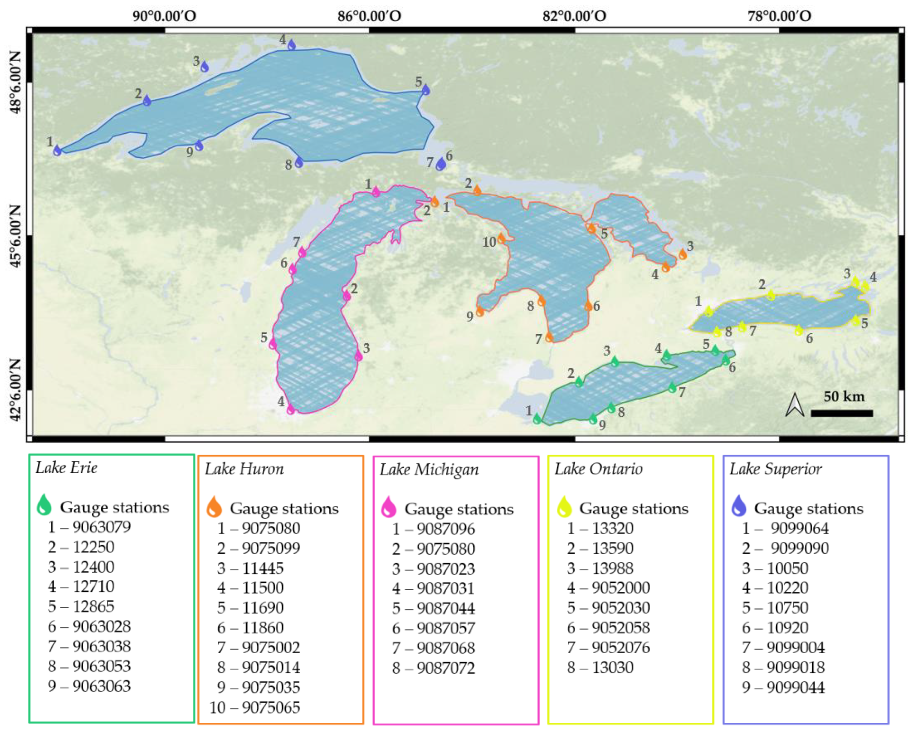
This paper is organized into five sections. A description of the studied lakes and datasets is given in Section 2. The results are given in Section 3, followed by a discussion in Section 4. Finally, the main conclusions are presented in the last section.

2. Study Areas and Datasets

2.1. Studied Lakes

The Great Lakes region is made up of large and deep interconnected surface freshwater systems in east–central North America. Along the border between the United States and Canada are the five main lakes: Erie, Huron, Ontario, Michigan, and Superior (Figure 1). By surface area, the Great Lakes represent the largest expanse of freshwater on Earth, spanning a total surface area of 244,106 km2. By volume, the Great Lakes system represents the second-largest volume, holding 21% of the world’s readily available surface freshwater. The surface areas of the studied lakes vary greatly between 19,010 km2 and 82,100 km2 (Table 1). Exceeding 50,000 km2, Lake Superior, Michigan, and Huron rank among the five largest lakes in the world, and the two remaining lakes have surface areas of approximately 20,000 km2. The average water level elevation for the majority of the lakes is between 174 and 183 m, while Lake Ontario has an average water level elevation of approximately 75 m. Table 1 presents the associated information about the five lakes.

2.2. Datasets

2.2.1. In Situ Water Levels from Gauging Stations

The water levels are continuously monitored by a network of 86 hydrometric coastal stations located throughout the Great Lakes shoreline and the connecting channels. The Canadian Hydrographic Service of Canada’s Department of Fisheries and Oceans operates the monitoring gauge stations located on the Canadian shoreline, and the NOAA’s Center for Operational Oceanographic Products and Services (CO-OPS) monitors the stations situated on the American side. Both CO-OPS (https://tidesandcurrents.noaa.gov/stations.html?type=Water+Levels, accessed on 14 March 2022) and the Fisheries and Oceans Department of Canada (https://www.qc.dfo-mpo.gc.ca/tides/en/tide-and-water-level-station-data, accessed on 14 March 2022) provide the historical water level records free of charge. In this study, the reference lake level data was acquired from 44 of the 86 in situ hydrometric stations. The non-retained hydrometric stations were located in the connecting channels, bays, and lakes located along the shoreline of the five main lakes. These stations do not exactly measure the water level of the lakes as they are generally separated from the rest of the lake by island chains or are influenced by the rhythm of the rivers flowing into the bay. For that reason, in order to reliably analyze the accuracy of the GEDI sensor, these stations have not been considered in the study.
The accuracy of the GEDI data is assessed in this study based on the similarity between the altimeter measurements from GEDI and the measurements recorded at the same time at the gauge station closest to a given GEDI acquisition date (Figure 2) within a maximum radius of 100 km. As shown in Figure 2, the footprints acquired on 31 October 2019, and composing a GEDI track spanning 260 km over Lake Erie, are compared to in situ measurements of five different gauge stations. Regarding the chosen 100 km maximum radius, it was shown (dashed rectangle in Figure 3) that the water level measurements are very close, with a difference not exceeding 5 cm on average. This observation led us to use the GEDI shots that are less than 100 km from a gauge station in this study, and thus avoid comparisons of measurements that are too far apart, which could strongly influence the evaluation of the accuracy of GEDI elevations.

2.2.2. GEDI Data Products

The NASA Global Ecosystem Dynamics Investigation (GEDI) is a spaceborne LiDAR instrument launched to the International Space Station (ISS) in late 2018. Since April 2019, the instrument produces high-quality measurements of surface vertical structures. The GEDI system records the amount of returned light energy emitted by a 1064 nm laser pulse with a PRF of 242 Hz reflected off by the ground, vegetation, and even clouds within a 25 m footprint. The collection of photons returned and collected by the LiDAR sensor are converted to an electronic voltage and recorded as a function of time in 1 ns (15 cm) intervals. A full waveform is the distribution of the recorded voltage (laser energy reflected) as a function of height above the ground. The waveform can be processed to provide height and profile metrics. The surface height is derived from two-way travel time of the electromagnetic wave multiplying it by the velocity of the light in vacuum and dividing it by two.
Different levels of products can be downloaded depending on the amount of processing applied to the data after collection. NASA’s Land Processes Distributed Active Archive Center (LP DAAC) processes and publishes all GEDI lower-level data products (Level 1 and Level 2), which include the geolocated raw waveforms, as collected by the GEDI system (L1B), footprint-level elevation and canopy heights metrics (L2A), and the footprint-level canopy cover and vertical profile metrics (L2B). In this study, from Version 2 of the L1B data product, we extracted the received waveforms, their geolocation (longitude and latitude), as well as their acquisition time. In addition, from the L2A data product, we extracted the following variables derived from the processing algorithm 1 (based on the ‘selected_algorithm’ variable from the L2A data product): (1) the latitude, longitude, and elevation of the lowest mode; (2) the latitude, longitude, and elevation of the instrument; (3) the number of detected modes (num_detectedmodes); (4) the width of the Gaussian fit to the received waveform (rx_gwidth); (5) the amplitude of the smoothed waveforms lowest detected mode (zcross_amp); (6) the viewing angle (VA) at acquisition time [14]; finally, (7) the signal to noise ratio (SNR) [14].

2.2.3. Transformation of Elevations

The geolocated elevations of the GEDI waveforms collected by the LiDAR system were relative to the WGS 84 ellipsoid. The water height collected by the gauge stations on the Great Lakes were referenced to the International Great Lakes Datum 1985 (IGLD 85). When comparing these datasets, GEDI elevations and lake level heights needed to be referenced through the same vertical datum. Consequently, the elevations provided by GEDI and water heights from gauge stations were converted to the North American Vertical Datum 1988 (NAVD 88). The conversion of the water-level stations data between the IGLD 85 and the NAVD 88 was conducted through NOAA’s National Geodetic Survey (NGS) online transformation tool (https://geodesy.noaa.gov/cgi-bin/IGLD85/IGLD85.prl#FILE, accessed on 14 March 2022). For GEDI elevations, the web application ‘Vdatum’ was used to vertically transform the WGS 84 ellipsoidal heights to NAVD 88 (https://vdatum.noaa.gov/, accessed on 14 March 2022).

2.2.4. Filtering the GEDI Waveforms

The quality of LiDAR returns is strongly degraded by transmission, absorption, and scattering in the atmosphere due to the presence of clouds, water (vapor and meteor), and aerosols [19,20], as such, some GEDI acquisitions are unusable. Consequently, four filtering operations were performed to remove those lower quality GEDI returns. Focusing our interest on measurements acquired over only water surfaces, the first filtering consists of the removal of all waveforms with more than a single energy peak (multimodal data). Waveforms that show multiple modes are characteristic of GEDI footprints, including complex geometries, while over flat surfaces, such as over water, GEDI waveforms exhibit a single mode. The second filter consists of eliminating all waveforms that report elevations much higher than the corresponding 30 m Shuttle Radar Topography Mission (SRTM) elevations. The GEDI acquisitions reporting elevations that exceeded the SRTM measurements by 50 m were not considered in the dataset. In fact, these GEDI acquisitions generally correspond to the elevation of clouds hit by the GEDI laser beam. Finally, two filters based on the median of absolute deviations (MAD) were used in order to minimize the potential impact of the residual outliers [21]. The third filter was computed over each track (acquired shots along a given beam on a given date) of GEDI measurements ( G E D I T ) by first calculating the median of all GEDI elevations along each track ( M T ). Next, the absolute deviation from the median was calculated for each GEDI shot along each track ( A D T = | G E D I T M T | ), followed by the median of absolute deviations ( M A D t = m e d i a n ( A D T ) , and finally the standard deviations ( σ T = 1.4826 M A D T ) were calculated. Only GEDI measurements within the range of [ M T 2 σ T ,   M T + 2 σ T ] were retained at this stage. Next, given that the M A D T filter removes some GEDI shots by comparing them to same-track acquisitions (outliers), some tracks affected by atmospheric conditions could exhibit a very high bias (higher than ±5 m) in comparison with acquisitions from other tracks. In order to remove such tracks, a fourth filter, also based on MAD, was applied. This last filter was calculated over all GEDI measurements from all the tracks ( G E D I A ), where the median of all GEDI elevations was first calculated ( M A ). Next the absolute deviation from the median of each measured elevation was then calculated ( A D A ), followed by the median of absolute deviations ( M A D A ) and the standard deviation ( σ A = 1.4826 M A D A ). Finally, GEDI measurements within the range of [ M A 5 σ A ,   M A + 5 σ A ] were retained.
Over the five studied lakes, 14.27 million GEDI acquisitions were available with 85.6% of viable acquisitions.

2.2.5. Geostationary Operational Environmental Satellites (GOES)

As mentioned earlier, three types of factors (instrumental, atmospheric, and water surface state) were utilized in the error budget models in order to correct GEDI water level estimates. Regarding the atmospheric factors, we used atmospheric variables from the Geostationary Operational Environmental Satellite-R series (GOES-R). GOES-R is the latest generation of geostationary satellites, with its first launch in November 2016 (became GOES-16 when it achieved geostationary orbit). GOES-R continually monitors the Western Hemisphere from approximately 36,000 km above the Earth. Onboard GEOS-R is an advanced baseline imager (ABI) instrument. The ABI comprises a 16-band radiometer, with spectral bands covering the visible, near-infrared, and infrared portions of the electromagnetic spectrum [22]. From ABI data, many higher-level-derived products can be generated and used in a large number of environmental applications [22]. In this study, five cloud (C) products from the full-resolution cloud and moisture imager (CMI) products (Level 2) were used (https://docs.opendata.aws/noaa-goes16/cics-readme.html#about-the-data, last accessed on 20 April 2022):
  • Clear sky mask (CSM): The main purpose of the CSM product is to distinguish between cloudy (pixel value of 1) and clear pixels (pixel value of 0) in a satellite scene at each GEDI acquisition. CSM data are available at a resolution of 2 km over the CONUS at a temporal resolution of 5 min.
  • Cloud type (CT): The cloud type product is used to classify the dominant cloud types and contains 10 classes. CT data are available at a resolution of 2 km over the CONUS at a temporal resolution of 5 min.
  • Cloud top temperatures and heights (CTT and CTH, respectively): The CTT and CTH products contain information regarding cloud top heights (CTH) and cloud top temperatures (CTT) for all the pixels identified as cloudy from the CSM product in a given satellite scene. Both CTT and CTH are available at a resolution of 5 km over the CONUS at a temporal resolution of 5 min.
  • Cloud optical depth (COD): The Cloud Optical Depth product contains an image with pixel values identifying the measure of the extinction due to condensed water or ice clouds at a wavelength of 0.64 um. COD data are available at a resolution of 2 km over the CONUS at a temporal resolution of 5 min.

2.2.6. Water Surface State Factors

Regarding the water surface state factors (W) used in the error budget models, they were downloaded from the National Oceanic and Atmospheric Administration (NOAA) Environmental Modelling Center (EMC) using the Great Lakes Wave model (GLWU) that is based on the 3rd generation wave model WAVEWATCH III (https://polar.ncep.noaa.gov/waves/index.php, last accessed on 20 April 2022). The GLWU was implemented on an unstructured grid with a spatial resolution of 0.25° × 0.25° and a temporal resolution of 1 h. A total of 12 factors were downloaded and used in this study:
  • Information on swell waves: Includes three variables—height, period, and direction.
  • Information on wind generated waves: Includes three variables—height, period, and direction.
  • Information on wind: Includes two variables—direction and speed.
  • Information on gusts: Includes two variables—direction and speed.
  • Water surface temperature.
  • Current direction.

3. Methodology

In order to improve the altimetric capabilities of GEDI acquisitions, we propose a series of models that estimate the difference between GEDI and in situ elevations by means of a random forest regressor (RF). These models take a given set of factors (e.g., instrumental, atmospheric, wave surface state) as input for each GEDI acquisition, and produce the estimated difference between GEDI and in situ elevations as output (i.e., the error). Adding the estimated error to the original GEDI elevation estimates thus produces a corrected GEDI elevation estimate.
Therefore, the proposed methodology could be separated into three parts. First, an assessment of GEDI elevation accuracy was made over the five Great Lakes over the period from April 2019 through October 2020. Second, several error budget models were proposed in order to reduce the inaccuracy (in terms of both the bias and random errors) on GEDI elevation estimates by accounting for one or more of the three sources of errors (namely instrumental, atmospheric, and water surface state). Third, the proposed models were assessed based on their ability to improve the accuracy of GEDI elevations over the spatial (training a correction model over a given lake and validating it over another lake) and temporal (training a correction model over a given year and applying it over another) domains, and as a function of available input factors (i.e., instrumental, atmospheric, and water surface state).
The choice to use RF was motivated by the fact that RF is able to mix quantitative and categorical variables, offers a measure of importance of the variables, and is known to be very performant [23]. Compared with linear models, RF is advantageous for being able to also model nonlinear relationships between the variable to explain and the explanatory variables. For this study, the number of trees in the RF was set to 500 trees, with a tree-depth equal set to the square root of the number of available factors.

3.1. Experimental Settings and Models Validation

3.1.1. Exploring Temporal Dependencies

In order to assess how our proposed model, which estimates the errors of GEDI’s elevation estimates, generalizes to future GEDI acquisitions for a given lake, model validation should be performed on data that are temporally far from the training data. Therefore, our first evaluation of the random forest regression model that uses the entirety of the factors (Instrumental I, Atmospheric C, and water surface state W) (Table 2) as predictors was based on splitting the dataset into two parts, the first part comprised acquisitions made in 2019 and the second comprised data acquired in 2020 (Table 3). As such, the model was trained over the 2019 dataset and validated on the 2020 dataset, and the process was repeated in reverse, where the model was trained on the 2020 dataset, and then validated on the 2019 dataset. This procedure was carried out for each lake independently. The choice to test the models on lake-by-lake basis was due the unequal number of GEDI acquisitions over the five lakes, for example, ~44% of acquisitions were taken over Lake Superior, while only ~7% of shots were acquired over each of Lake Erie and Lake Ontario. As such, by testing a single model using the combined data from all the lakes, the results would be biased towards the lake with the highest GEDI count, and intrinsic differences of the GEDI shots across the lakes might be lost.

3.1.2. Exploring GEDI Elevation Error Budget

The proposed models in Section 3.1.1 present a best-case scenario, where a large number of factors corresponding to instrumental, atmospheric, and water surface state for each GEDI footprint are present. Nonetheless, such large and rich dataset is hard to obtain for different lakes globally. Therefore, it is essential to test the loss of accuracy by omitting certain factors from the proposed model in Section 3.1.1 and reperforming the same training/validation test. In this study, as stated previously, the used factors were organized into three main categories. The first category are instrumental factors (I, Table 2), and these variables are available for all acquired GEDI shots. The second category are factors related to atmospheric conditions and cloud composition at acquisition time (C, Table 2). These variables, while harder to obtain than I, could be acquired from the different satellites orbiting around the Earth. Finally, water surface state factors (W, Table 2) are scarce, and are only available for heavily monitored water bodies, such as those presented in this study. Therefore, in this study, three variants of the random forest regression model were tested. The first model only used instrumental factors. The second model used instrumental and atmospheric factors. Finally, the third model used instrumental and water surface state factors. As with Section 3.1.1, model training/validation was based on the year of acquisition (i.e., model trained on data acquired in 2019 and validated on data acquired in 2020, and vice versa). Table 3 summarizes the models that were tested in this study.

3.1.3. Exploring Geographical Location Effect

To evaluate whether the proposed model could be transferred from a study region to another, a random-forest-based model using all the available factors (I, C, and W, Table 2) as predictors was independently trained on a given lake and validated on the remaining four (Table 3). Moreover, to assess the performance of the spatially transferred models, for each of the five lakes, an additional random forest model was trained and validated within the lake with fivefold cross-validation (CV). Moreover, for the fivefold cross-validation, two constraints were imposed: (1) footprints belonging to the same track were assigned exclusively to one of the data partitions (training or test) with the aim to avoid possible spatial bias in the evaluation procedure; (2) the tracks were chosen randomly from either the 2019 or 2020 datasets in order to reduce any potential errors due to temporal dependencies.

3.2. Models Performance Evaluation

Models performance was assessed using the mean difference (bias) between GEDI-derived elevation estimates (either original or corrected after application of models detailed in Section 3.1) and in situ elevations, the unbiased root mean squared error (ubRMSE), the root mean squared error (RMSE), and the coefficient of determination (R2). ubRMSE, RMSE, and R2 are defined as follows:
u b R M S E = 1 N i = 1 N ( P i O i ) 2 ( 1 N i = 1 N ( P i O i ) ) 2
R M S E = 1 N i = 1 N ( P i O i ) 2
R 2 = 1 i = 1 N ( O i P i ) 2 i = 1 N ( O i P ¯ ) 2
where O i is the observed value (in situ), P i is the predicted value (GEDI), P ¯ is the mean of the predicted values, and N is the sample size.
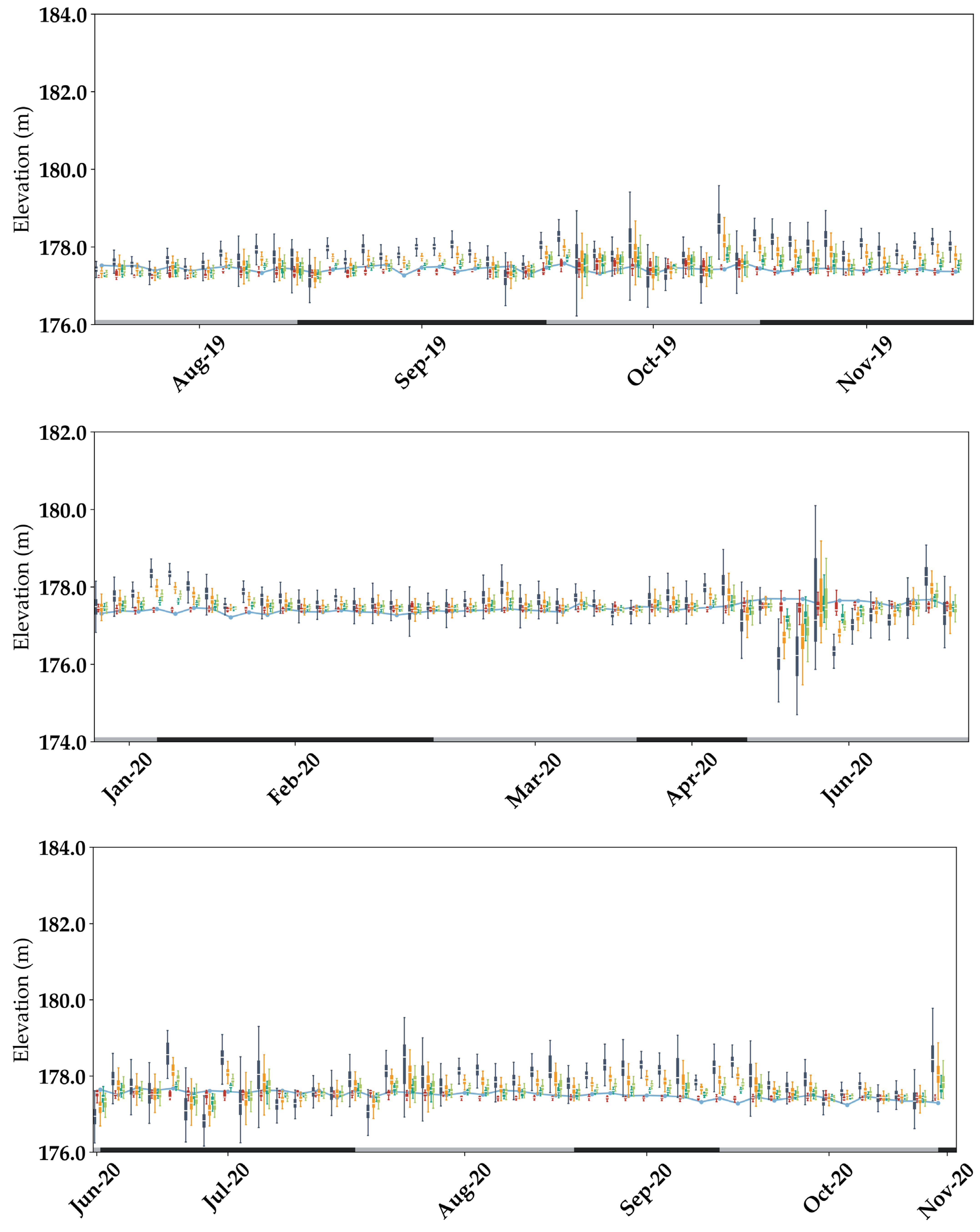
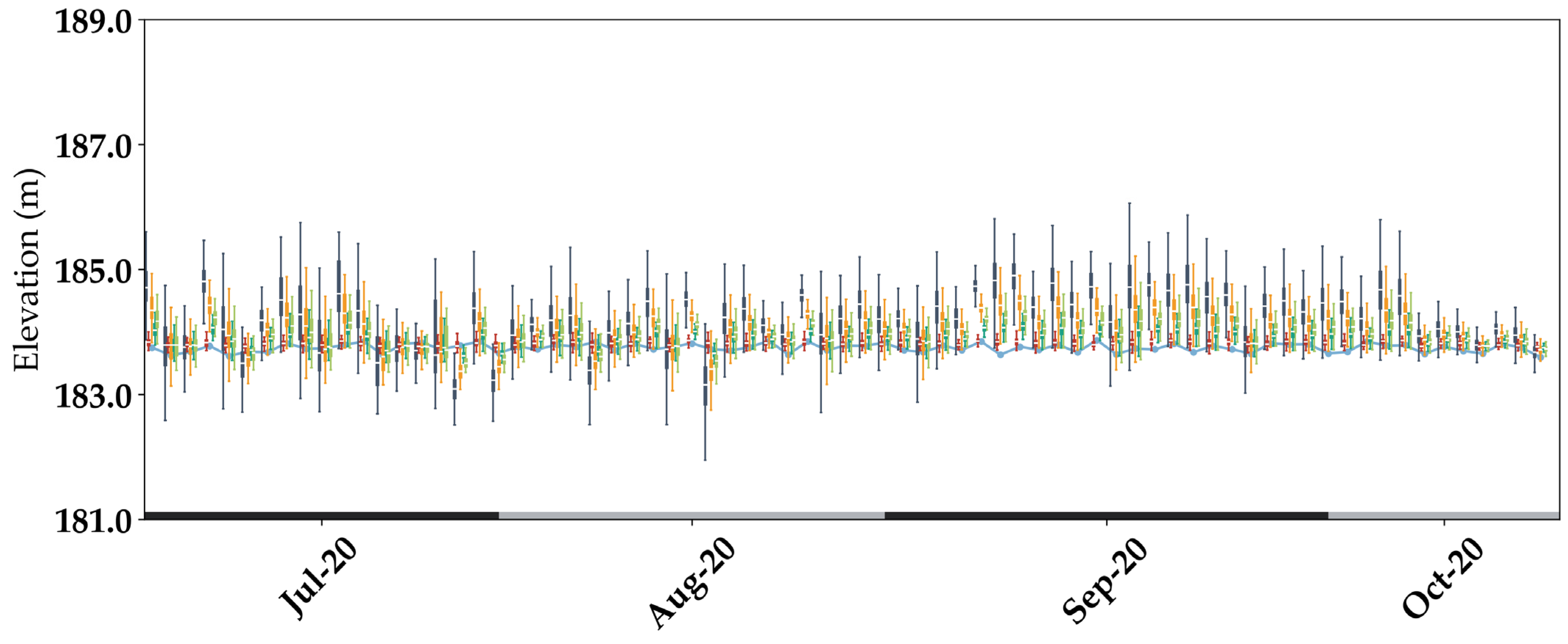
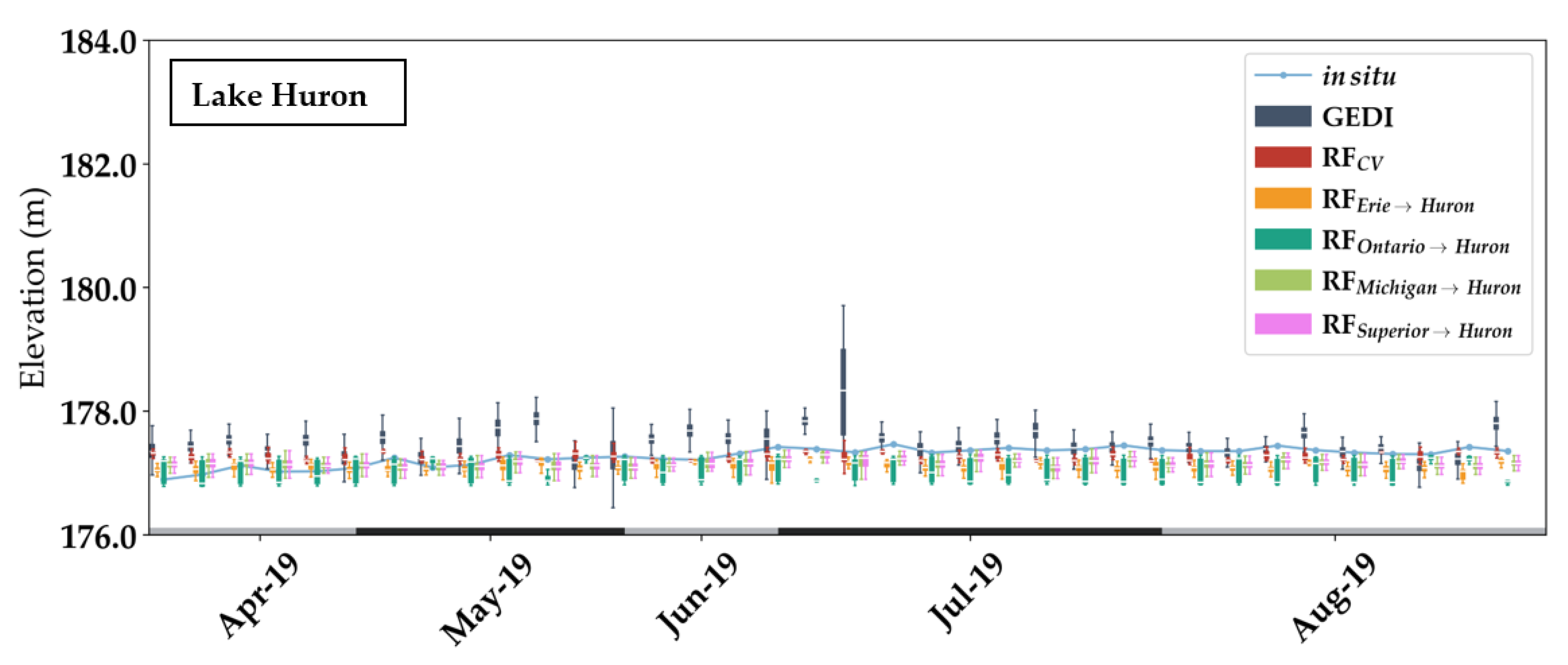
4. Results

4.1. Overall GEDI Elevation Estimates Accuracy

The accuracy of the GEDI elevation estimates was assessed for each lake separately. The distribution of the mean differences between GEDI and in situ elevations (bias) in Figure 4 shows that the bias was similar across the lakes. Indeed, ~45% of acquisitions (GEDI shots grouped by acquisition date and acquiring beam) had a bias between −0.4 m (underestimation) and 0.3 m (overestimation), and ~68% of acquisitions had a bias between −0.4 and 0.5 m. There were, however, acquisitions with large differences between the estimated GEDI and in situ elevations (either under- or overestimations, ( | bias | > 0.8   m ), and their percentage differed by lake. However, the percentage of these shots ranged between 10.8% of viable GEDI shots (Lake Erie) and 13.6% of viable GEDI shots (Lake Huron). Regarding the underestimation case, Lake Erie have acquisitions over seven dates (Figure A1) where GEDI elevation differences from in situ elevations were lower than −0.8 m, with a maximum difference between GEDI and in situ elevations of −1.8 m. Over Lake Ontario, 13 acquisition dates (Figure A1) showed a bias of less than −0.8 m, with a maximum difference to in situ data of −3.0 m. For Lake Michigan, there were 28 acquisition dates (Figure A1), where the difference between GEDI and in situ elevations was lower than −0.8 m, with a maximum difference between GEDI and in situ elevations of −3.0 m. Over Lake Superior, 34 acquisition dates (Figure A1) have a difference from in situ elevations lower than −0.8 m, with a maximum difference lower than −2.32 m. Finally, over Lake Huron, 21 acquisition dates (Figure A1) had a difference to in situ elevations lower than −0.8 m, with a maximum difference lower than −4 m. Regarding the over-estimation case, Lakes Erie, Huron, Michigan, Ontario, and Superior had 10, 20, 19, 11, and 29 acquisition dates (Figure A1), respectively, where the bias was higher than 0.8 m. Moreover, the highest difference ranged between 2.6 m (Lake Erie) and 3.9 m (Lake Huron).
Regarding the unbiased root mean squared error (ubRMSE), Figure 5 shows that the distribution of ubRMSE values was similar across lakes Erie, Huron, and Michigan. For these three lakes, the distribution of ubRMSE was lower than 0.3 m for more than 95% of all the tracks (a track corresponds to multiple GEDI shots acquired on the same date and with the same beam). For Lake Ontario, the distribution of ubRMSE was lower than 0.3 m for 92.8% of acquisitions, while for Lake Superior, 87% of the shots had a ubRMSE less than 0.3 m. Finally, there were only three acquisition dates (two over Lake Huron and one over Lake Michigan) where the ubRMSE was higher than 1 m (Figure A1).
In terms of RMSE (Figure 6), GEDI tracks had similar RMSE distributions on the estimation of water surface elevations across the five lakes. Moreover, ~50% of acquisitions had an RMSE ranging between 0 and 0.4 m, and ~80% of acquisitions had an RMSE in the range [0 m, 0.7 m]. The overall RMSE (calculated over all GEDI shots for each lake) ranged between 0.57 m (Lakes Erie and Superior) and 0.68 m (Lake Ontario).

4.2. Modeling of Elevation Errors Using R F I C W

In this section, the results of the models introduced in Section 3.1.1 (namely R F I C W , Table 3) are presented. The results show that, qualitatively, the model was able to improve the quality of GEDI elevations (Figure 7, GEDI vs. R F I C W ). The boxplots representing corrected GEDI elevations from the R F I C W model over Lake Huron (Results for the remaining Lakes can be found in Appendix B) have a median that is closer to in situ elevations in comparison with the original GEDI elevations estimates (Figure 7, GEDI). Moreover, boxplots from the R F I C W model are also smaller (i.e., smaller variations) in comparison with the original GEDI elevation estimates.
This is especially noticeable for the original acquisitions with a high bias and ubRMSE (e.g., July and October through December 2019, and March and June through July 2020, Figure 7 GEDI vs.   R F I C W ). Quantitatively, the distribution of the bias presented in Figure 8 shows that the R F I C W elevations were similar for acquisitions made in 2019 (trained on 2020 data) and those obtained in 2020 (trained on 2019 data). Moreover, for Lakes Huron, Ontario, and Michigan, most of the bias ranged between −0.20 and 0.20 m. In addition, for Lakes Huron and Ontario, 20% of GEDI acquisitions made in 2020 over Lake Huron were underestimated, with a bias ranging between −0.40 and −0.20 m, while ~25% of elevations were overestimated for Lake Ontario, with a bias ranging between 0.20 and 0.40 m. For Lake Erie, the bias ranged between −0.40 and 0.20 m, with a small percentage of acquisitions having a bias between 0.20 and 0.40 m. Finally, over Lake Superior, the corrected elevations acquired in 2019 ( R F I C W   20 19 ) mostly had a bias that ranged between −0.20 and 0 m, while corrected elevations that were acquired in 2020 ( R F I C W   19 20 ) had a bias that ranged between 0 and 0.20 m. Overall, for the five lakes, the bias of corrected elevations acquired in 2019 ranged between −0.06 and 0.09 m, and between 0.02 and 0.10 m for elevations acquired in 2020. The ubRMSE for the majority of corrected acquisitions of the five lakes was lower than 0.10 m, while some acquisitions, especially those acquired in 2020 ( R F I C W   20 19 , Figure 9), had a ubRMSE between 0.10 and 0.20 m for Lake Erie (16.1% of viable GEDI shots) and Lake Ontario (7.6%). Finally, in terms of RMSE, the majority of corrected GEDI elevation estimates (Figure 10) for Lakes Huron (85.7% for 2019 and 75.6% for 2020), Michigan (81.2% for 2019 and 93.5% for 2020), and Superior (81.1% for 2019 and 82.1% for 2020) were less than 0.20 m for both acquisition years ( R F I C W   20 19 , R F I C W   19 20 , Figure 10). For Lakes Erie and Ontario, the corrected GEDI elevation estimates were less precise, with ~42% of acquisitions (for both 2019, and 2020) having an RMSE between 0.20 and 0.40 m over Lake Erie, while for Lake Ontario, 20.0% of 2019 acquisitions and 29.5% of 2020 acquisitions had an RMSE between 0.20 and 0.40 m (Figure 10). Overall, the RMSE values for the estimation of in situ elevations using the R F I C W   20 19 model were 0.19 m (0.22 m for R F I C W   19 20 model), 0.14 m (0.21 m), 0.31 m (0.25 m), 0.16 m (0.12 m), and 0.15 m (0.15 m) for lakes Erie, Huron, Ontario, Michigan, and Superior, respectively.

4.3. Modelling of Elevation Errors Using R F I , R F I C , and R F I W

To analyze the factor effects on the accuracy of corrected GEDI elevation estimates, the three models presented in Section 3.1.3 for the correction of GEDI elevation estimates (using, separately: instrumental factors; both instrumental and atmospheric factors; and both instrumental and water surface state factors) were tested. Figure 7 shows that over Lake Huron, the model trained using only the instrumental factors ( R F I ) (i.e., VA, SNR, A, and gwidth) was the least accurate model in estimating GEDI’s elevation errors. However, the R F I model showed median values and variations that were better than the original GEDI elevation estimates (GEDI, Figure 7). The models trained using either instrumental and atmospheric factors ( R F I C ) or instrumental and water surface state factors ( R F I W ) shown in Figure 7 are boxplots of corrected GEDI elevations with similar median values and interquartile ranges. However, R F I C appears to be slightly more accurate. Quantitatively, in terms of bias (Figure 11), the three models ( R F I , R F I C , and R F I W ) had a larger range of bias values than that of the R F I C W model, ranging from −0.6 to 0.8 m across the five lakes. Nonetheless, the R F I C model had fewer GEDI acquisitions with bias values between 0.2 and 0.4 m (16.3% of acquisitions) and between 0.4 and 0.6 (2.3% of acquisitions) compared with the R F I W model (24.8% of acquisitions between 0.2 and 0.4 m and 6.0% between 0.4 and 0.6 m) and the R F I model (28.16% of acquisitions between 0.2 and 0.4 m, and 13.6% of shots between 0.4 and 0.6 m).
In terms of ubRMSE (Figure 12), the accuracy of R F I C showed similar performance to the full model ( R F I C W ), where the majority of shots had a ubRMSE in the [0 m, 0.10 m] range. The ubRMSE in the [0.10 m, 0.20 m] range corresponded to a maximum of 17.0% of tracks (case of Lake Ontario). The R F I W model was slightly less accurate than the R F I C model, with a lower percentage of tracks (GEDI shots acquired on the same date with the same beam) with a ubRMSE in the [0 m, 0.10 m] range. Finally, the R F I model was the least accurate between the four models with a percentage of shots having a ubRMSE between 0 and 0.10 m, ranging between 50.1 and 65.6% depending on the lake. In terms of RMSE, Table 4 shows that the lowest RMSE corresponded to results obtained with the R F I C W model followed by the R F I C model and then the R F I W model. The R F I model showed the highest RMSE values between the four tested models. Nonetheless, a significant improvement on GEDI elevation estimation was obtained with the R F I model in comparison with the original GEDI elevation estimates (decrease in RMSE by around 40% with the R F I model). Indeed, the R F I C model showed an RMSE that ranged between 0.19 and 0.24 m for Lakes Erie, Huron, Michigan, and Superior, and 0.30 m over Lake Ontario, while the RMSE on the elevation estimates using the R F I W model was 0.38 m for Lake Ontario, and was between 0.27 and 0.26 m for the remaining four Lakes. Finally, the R F I model showed an RMSE ranging between 0.35 and 0.45 m (Table 4). Finally, regarding the models coefficient of determination (R2) on the estimation of the error budget (i.e., the difference between GEDI and in situ elevation estimates), the results presented in Table 4 show that the R F I C W model had the highest explained variance with an R2 that ranged between 0.74 (Lake Ontario) and 0.92 (Lake Michigan). For the model using only instrumental and atmospheric variables ( R F I C ), a small decrease was observed in R2 in comparison with R F I C W , with R2 ranging between 0.70 (Lake Ontario) and 0.89 (Lake Michigan). Finally, with the instrumental-only model ( R F I ), only 0.37 (Lake Erie)–0.54 (Lake Michigan) of the error budget variance could be explained (Table 4).

4.4. Analysis of Spatial Independence on the Corrected GEDI Elevations

Table 5 (bias), Table 6 (ubRMSE), Table 7 (RMSE), and Table 8 (R2 on the estimated error budget) assess the precision of each of the five models that were trained on a given lake and validated on the remaining four. The results show that models trained over Lakes Huron (~2.25 M GEDI shots), Michigan (~2.1 M GEDI shots), and Superior (~4.84 M GEDI shots) provide the best correction of GEDI elevation estimates, with a bias ranging between −0.03 and 0.15 m for Lake Huron, between −0.01 and 0.04 m for Lake Michigan, and between −0.03 and 0.07 m for Lake Superior. For these three lakes, the ubRMSE (m) (Table 6) ranged between 0.14 and 0.21 m (resp. RMSE between 0.15 and 0.24 m) for Lake Huron, between 0.17 and 0.20 m (resp. RMSE between 0.16 and 0.21 m, Table 7) with Lake Michigan, and between 0.15 and 0.19 m with Lake Superior (resp. RMSE between 0.16 and 0.21 m, Table 7). Error budget explained variance (R2) ranged between 0.84 and 0.93 for Lake Huron, between 0.86 and 0.93 for Lake Huron, and between 0.86 and 0.91 for Lake Superior. Finally, Lakes Erie (~0.88 M GEDI shots) and Ontario (~0.89 M GEDI shots) show the lowest generalization accuracy with a bias (Table 5) that ranged between 0 and 0.12 m for Lake Erie and between 0.05 and 0.16 m for Lake Ontario, with a ubRMSE ranging between 0.19 and 0.29 m (Lake Erie) and between 0.16 and 0.24 m (Lake Ontario) (Table 6). Finally, the RMSE (resp. R2) of the models trained on Lakes Erie and Ontario ranged between 0.20 and 0.29 m (R2 between 0.76 and 0.88) and between 0.17 and 0.29 m (R2 between 0.63 and 0.85) (Table 7), respectively.
Overall, the models that provided the best generalizability provided accuracies on the corrected GEDI elevations that were very close to the fivefold cross-validation results. Indeed, when validated across the four other lakes, a model trained on Lake Huron showed a difference in RMSE in comparison with the respective fivefold cross-validation models that ranged between 0.03 m (RMSE of 0.17 m over Erie using the model trained over Huron vs. 0.14 m with the CV model over Lake Erie; Table 7) and 0.08 m (RMSE of 0.18 m over Superior using the model trained over Huron vs. 0.10 m with the CV model over Lake Superior; Table 7). Similar accuracies were obtained with models trained over Lakes Michigan or Superior and the respective fivefold cross-validated models (difference in RMSE lower than 0.09 m) (Table 7). Moreover, a model trained over Lake Huron (RMSE = 0.24 m) provided better accuracies on the GEDI elevation estimates over Lake Ontario than the fivefold cross-validated Lake Ontario model (RMSE = 0.28 m) (Table 7). Regarding the performance of the models trained over Lakes Erie or Ontario, the difference between the accuracies obtained with these models and the respective fivefold cross-validated models ranged between 0 and 0.17 m for a model trained over Lake Erie, and between 0.02 and 0.18 m with a model trained over Lake Ontario (Table 7). In terms of R2, results in Table 8 show that the fivefold cross-validated models have an R2 that ranges between 0.82 (Lake Ontario) and 0.94 (Lake Huron), while the R2 from a model trained over a lake and validated on another (cross-lake validation) was slightly lower for all lake combinations, and the difference in explained variance between the fivefold cross-validated models and the cross-lake models was dependent on the lake used for training. For example, in the case of Lake Erie, a fivefold cross-validated model could explain 88% of the error budget variance, while the R2 of the cross-validated models ranged between 0.84 (Lake Huron) and 0.86 (Lakes Michigan and Superior). In contrast, in the case of Lake Ontario, a fivefold cross-validated model could only explain 82% of the error budget variance, while cross-lake models showed higher values (ranging between 0.85 and 0.91) except for a model trained over Lake Erie that explained only 75% of the error budget variance (Table 8). Boxplots tracking the original estimated elevations by GEDI over the five lakes and the five tested models presented in Section 3.1.3 can be found in Appendix C.

5. Discussion

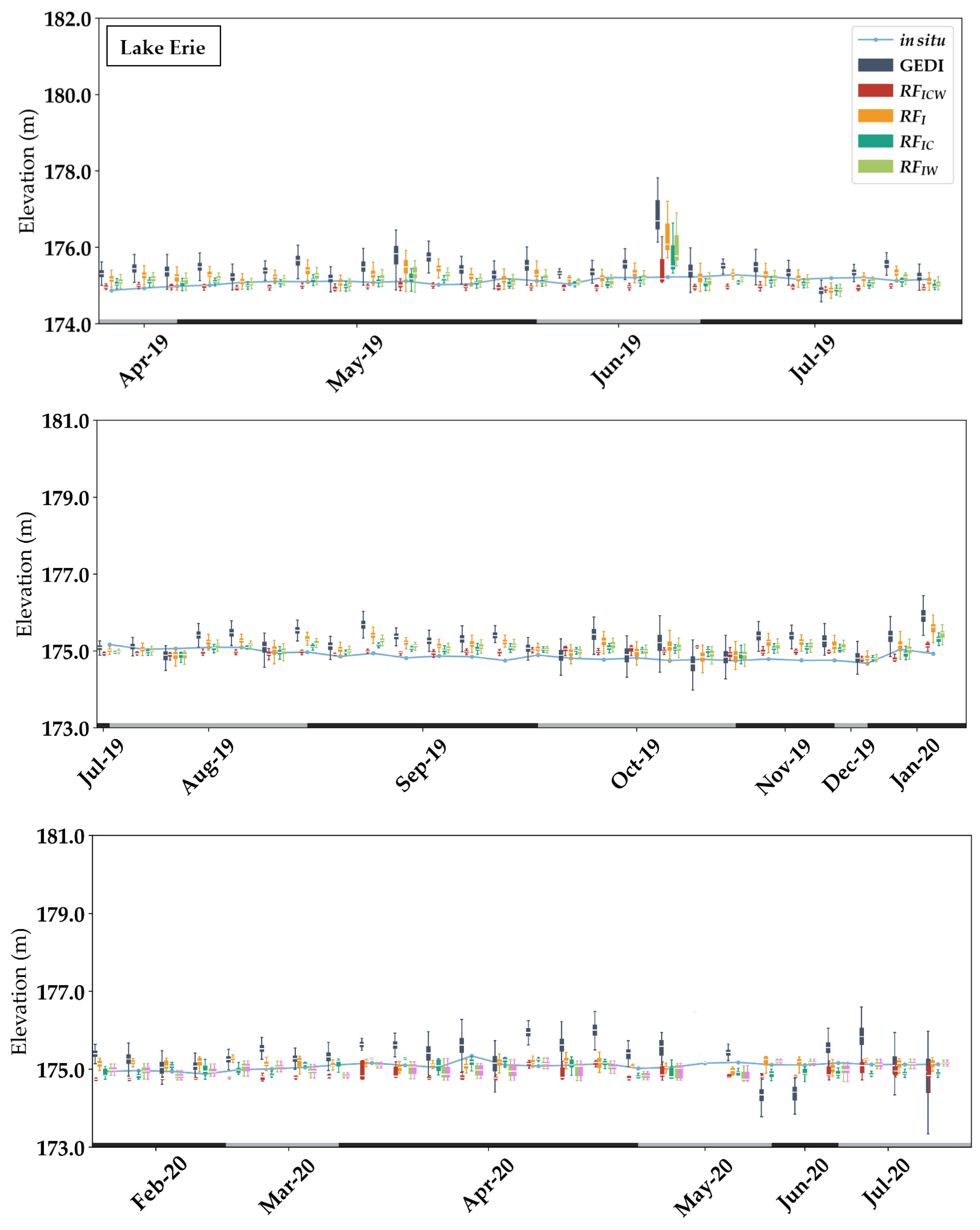
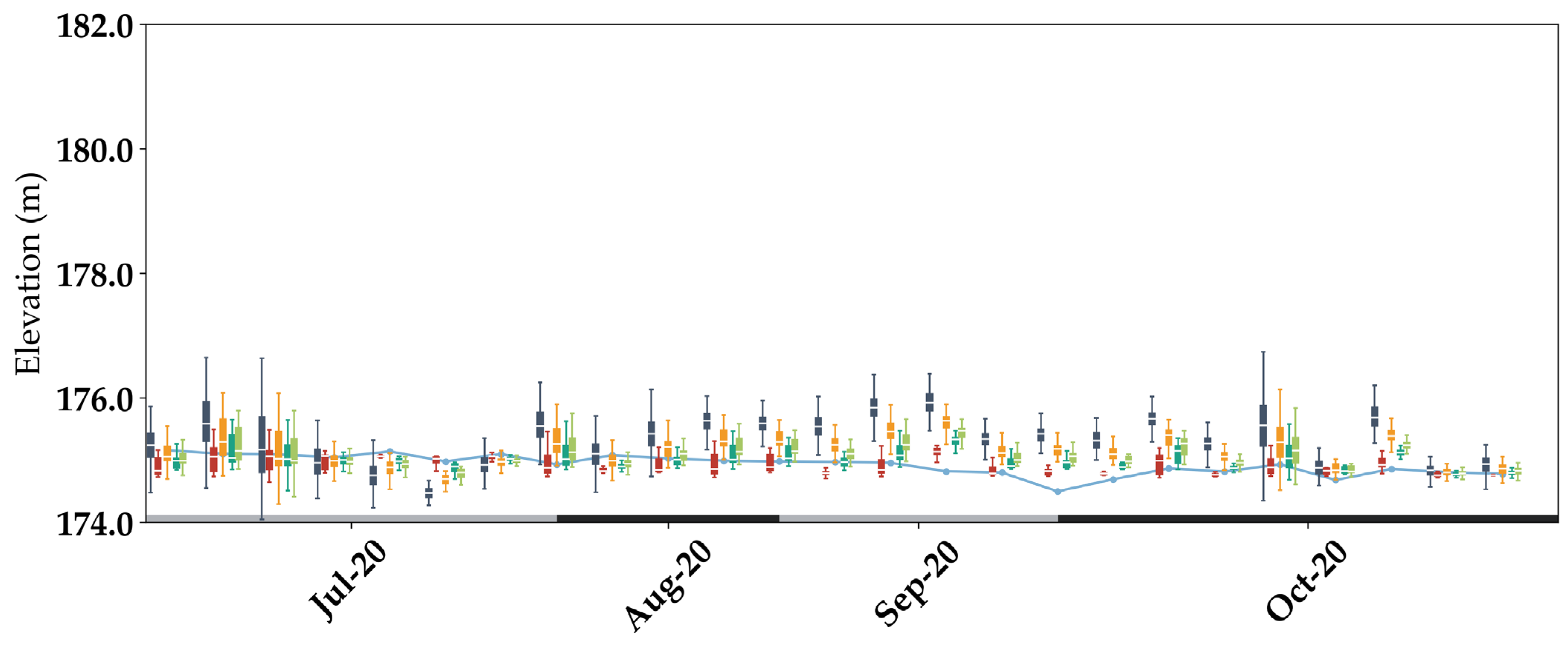
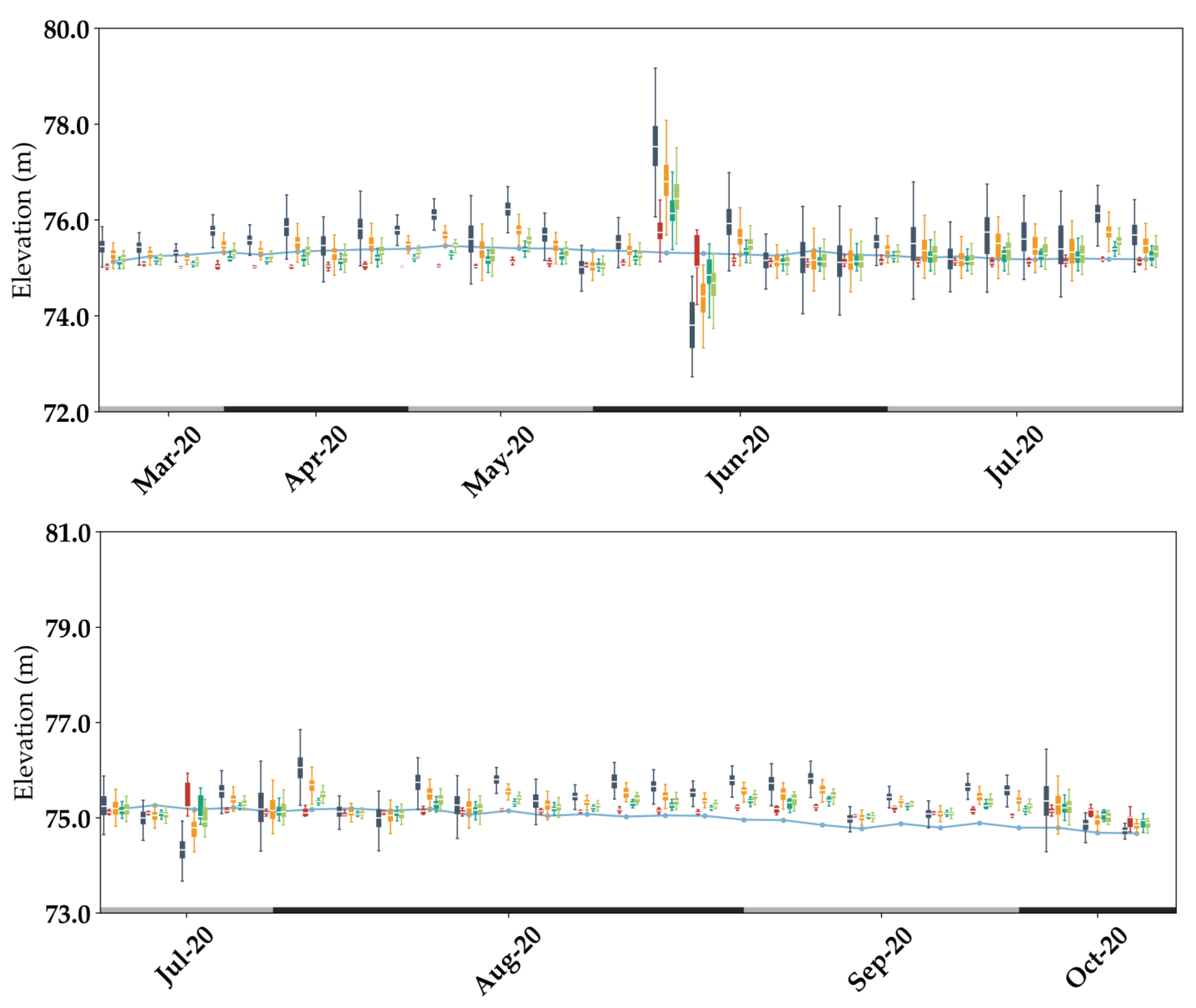
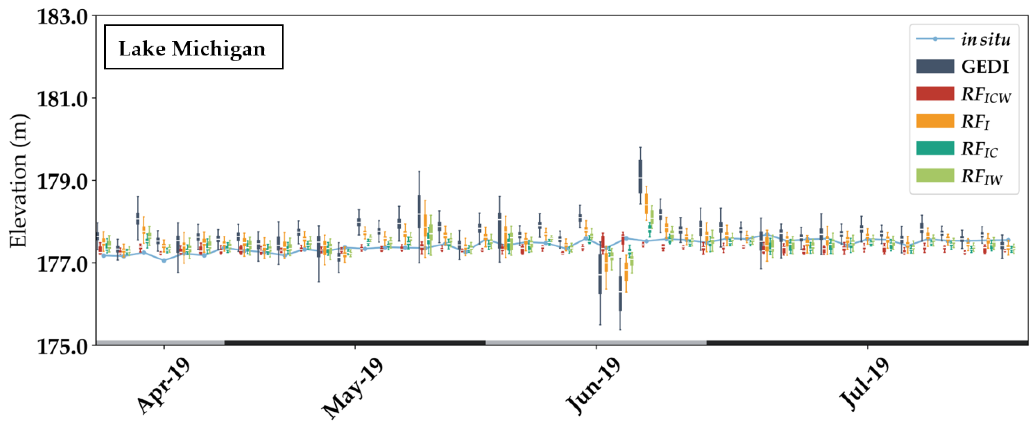
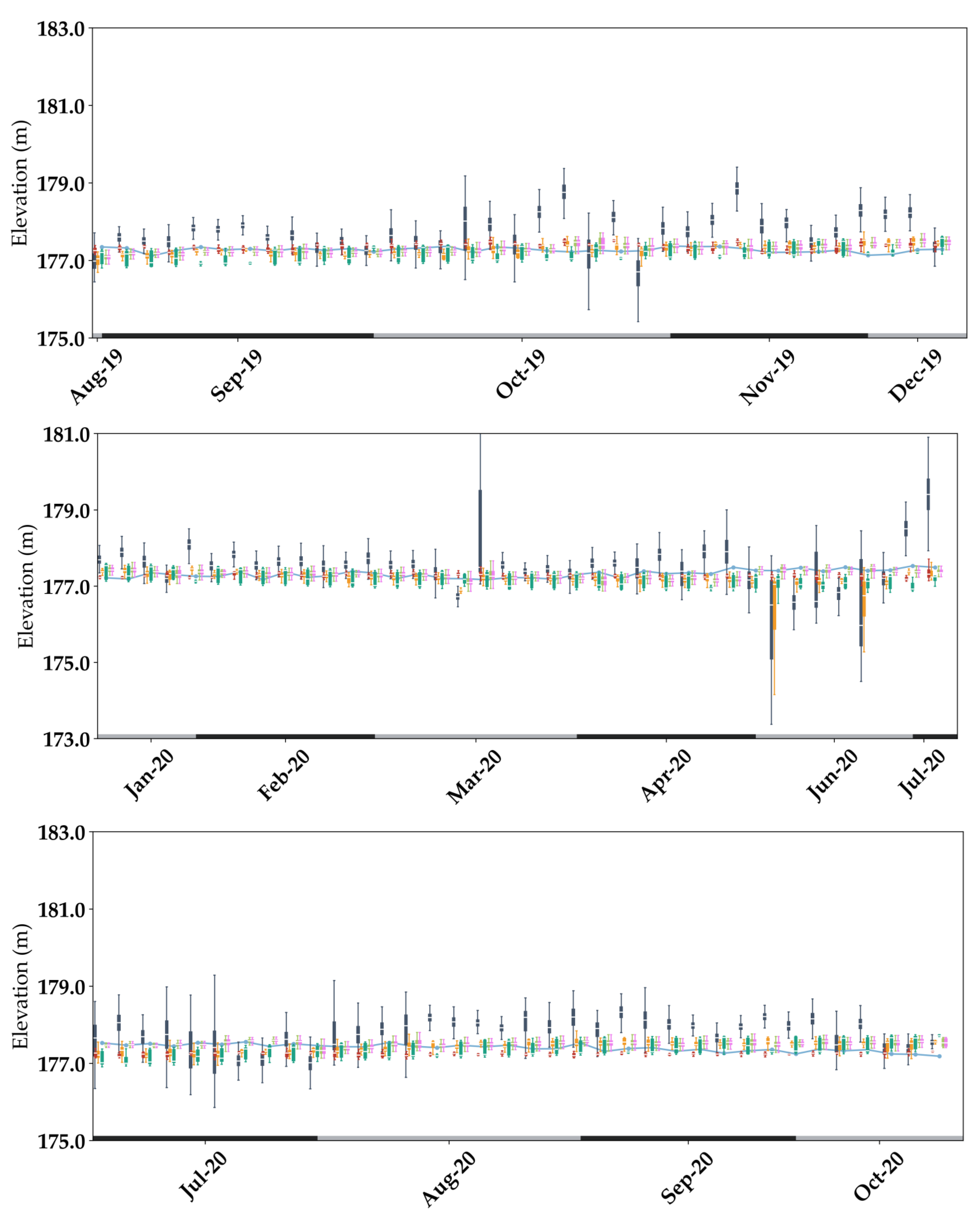
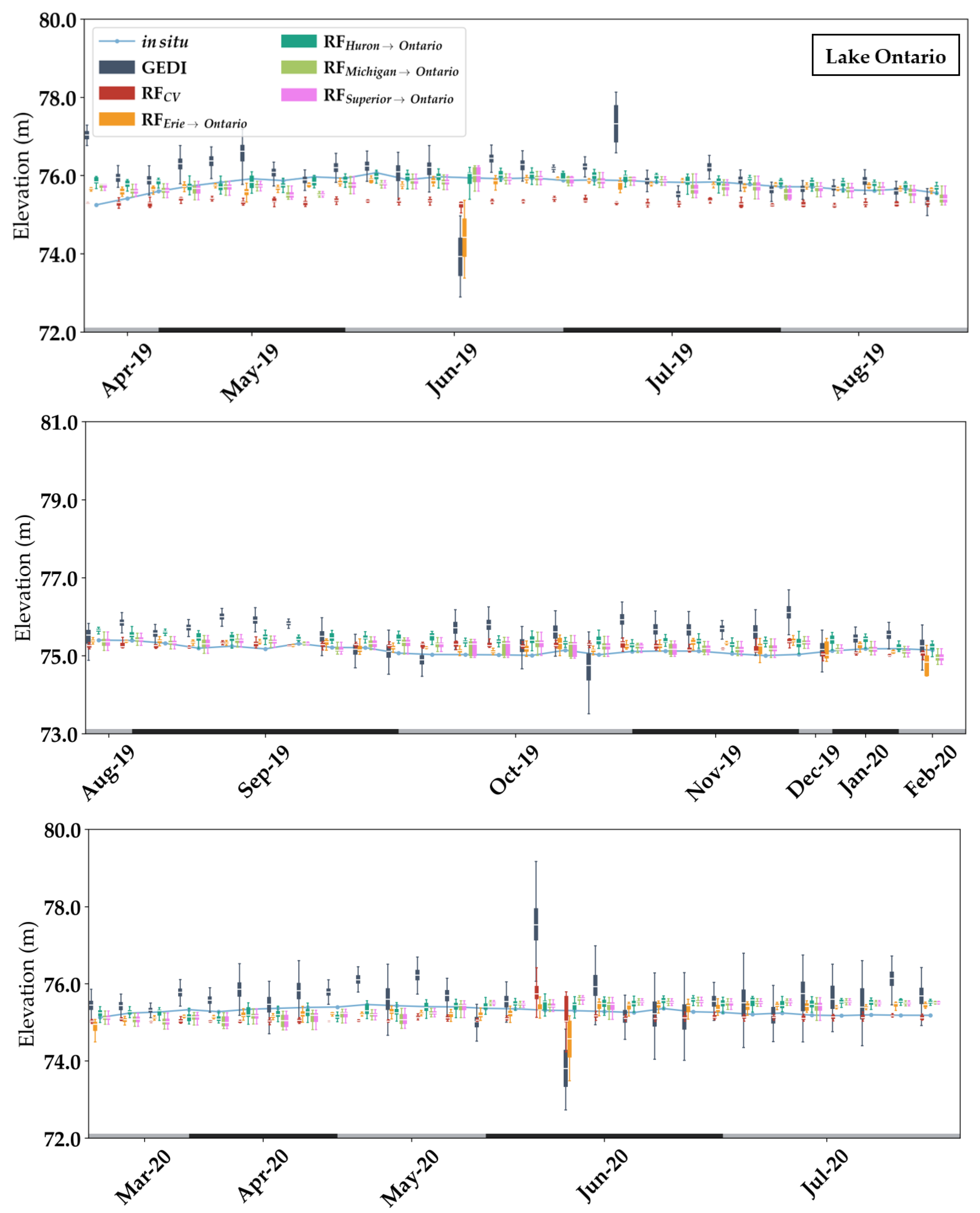
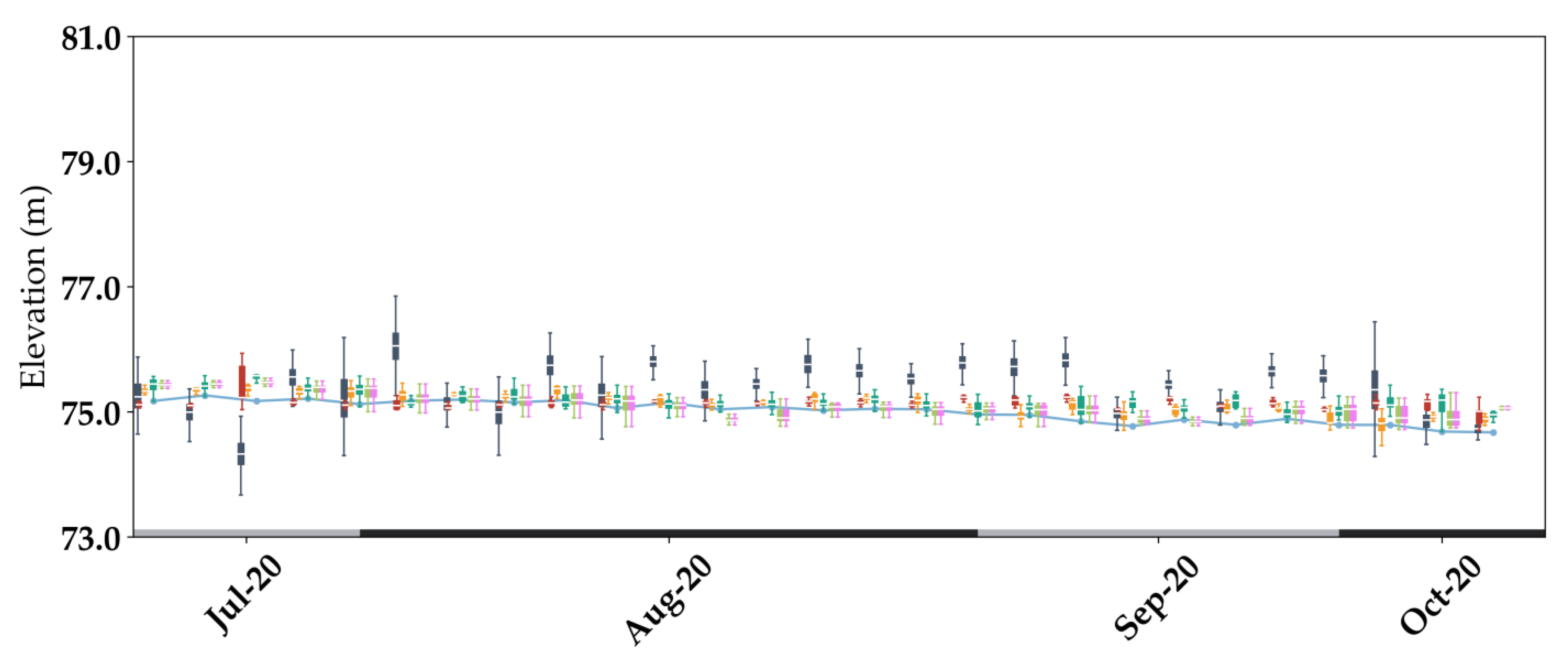
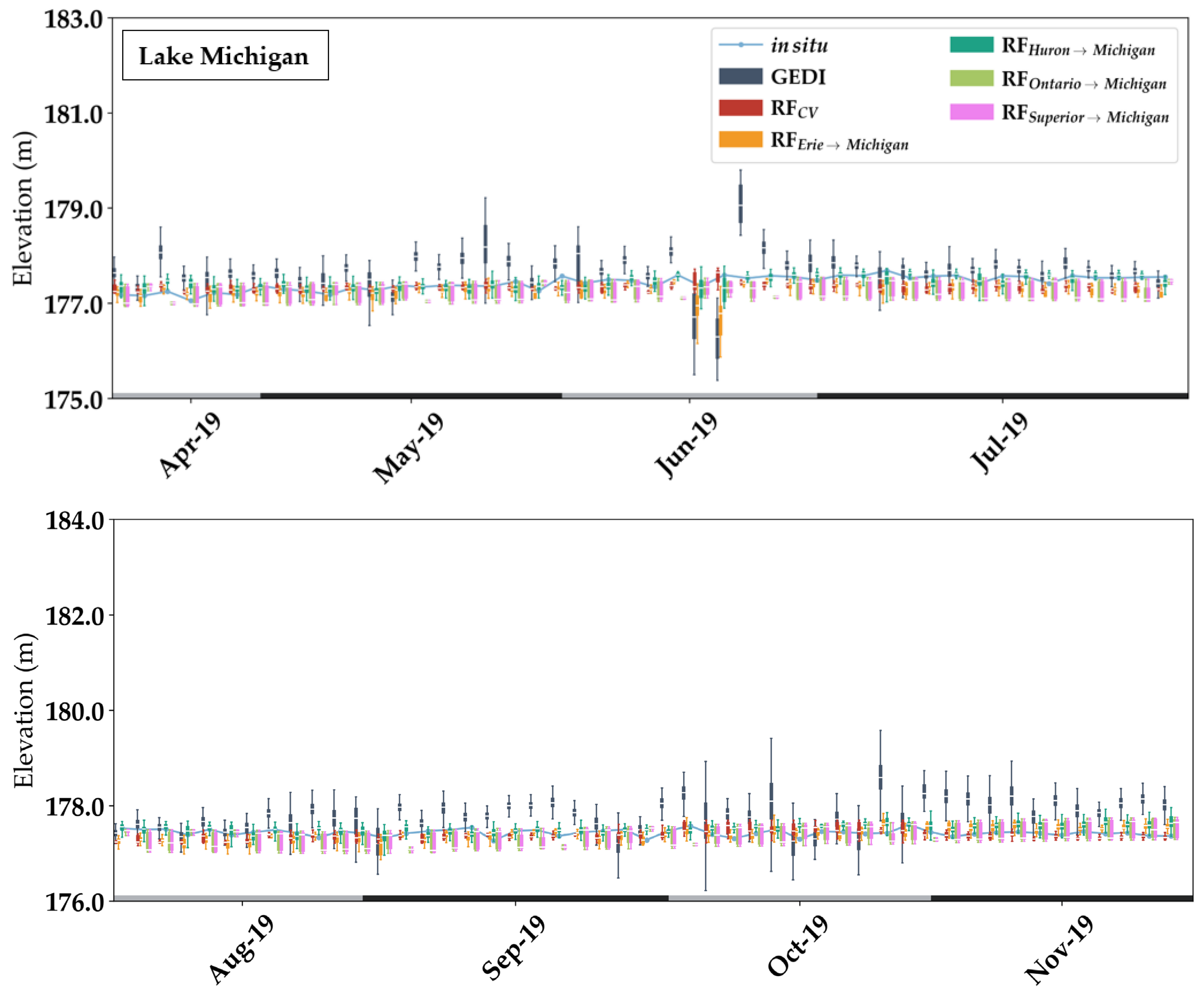
The results presented in this study show a severe limitation of uncorrected GEDI’s altimetric capabilities for the estimation of water levels. Indeed, from the 12 million GEDI shots acquired over a span of 18 months (April 2019 through October 2020), the assessed uncertainties of GEDI elevation estimates are three times higher than the worst performing radar retracker, namely the ERS-1 sea ice retracker, in the study of Shu et al. [3]. For example, with the ERS-1 sea ice retracker, the RMSE on the altimetry-derived water level estimates ranged from 0.25 m (Lake Superior) to 0.31 m (Lake Huron), with a bias ranging from 0.53 m (Lake Superior) to 0.78 m (Lake Superior). In contrast, with uncorrected GEDI estimates, the RMSE on the water level estimates ranged from 0.57 m (Lake Erie) to 0.68 m (Lake Ontario), with a bias that ranged from 0.43 m (Lake Erie) to 0.61 m (Lake Ontario). On the other hand, the uncertainties obtained with GEDI were consistent with other studies, such as the study of Xiang et al. [13] over the five Great Lakes, or the studies of Fayad et al. [14,18] and the study of Frappart et al. [6] over several lakes in France and Switzerland. Therefore, model-free GEDI elevation estimates are not recommended for the retrieval of water surface levels.
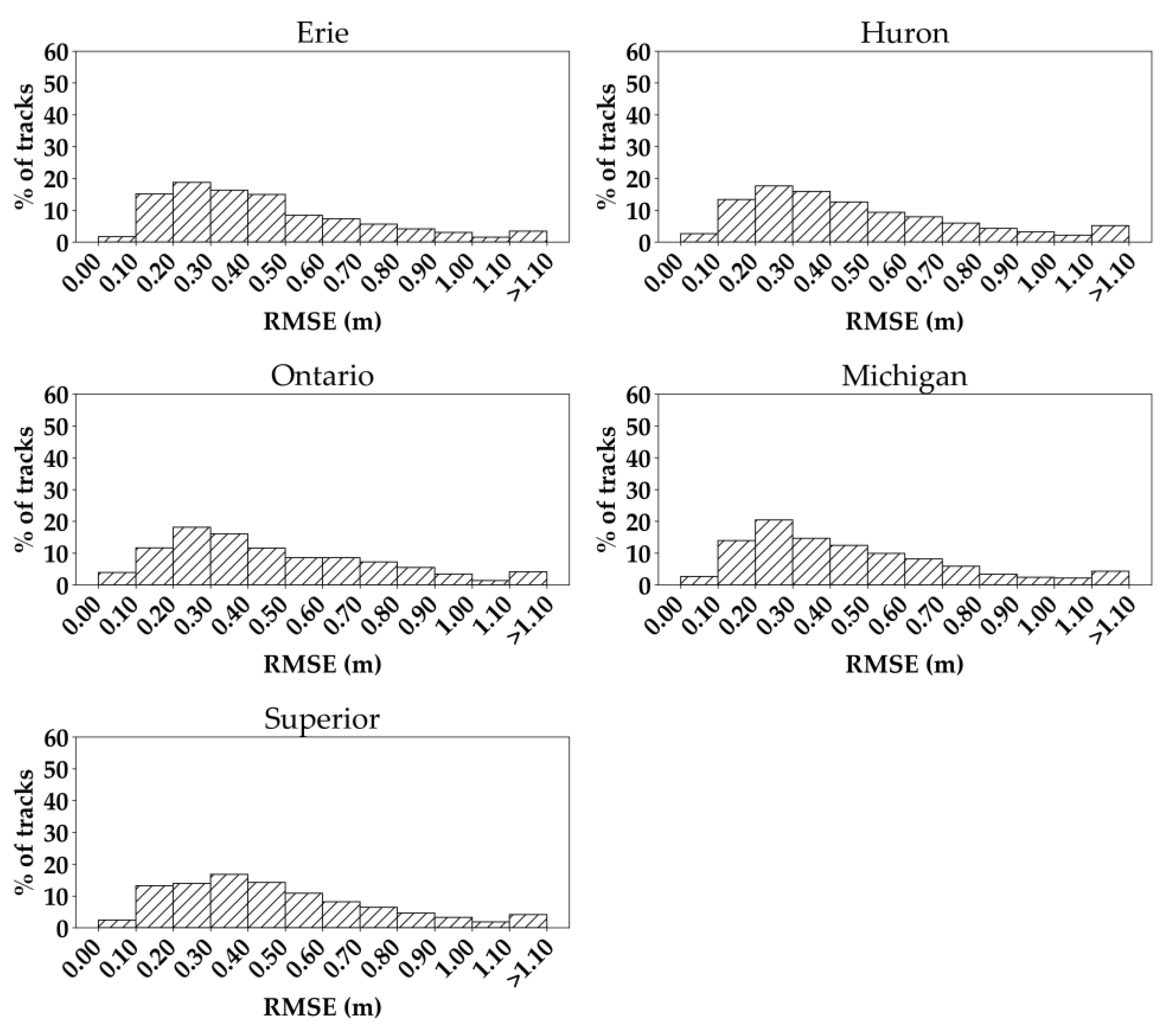
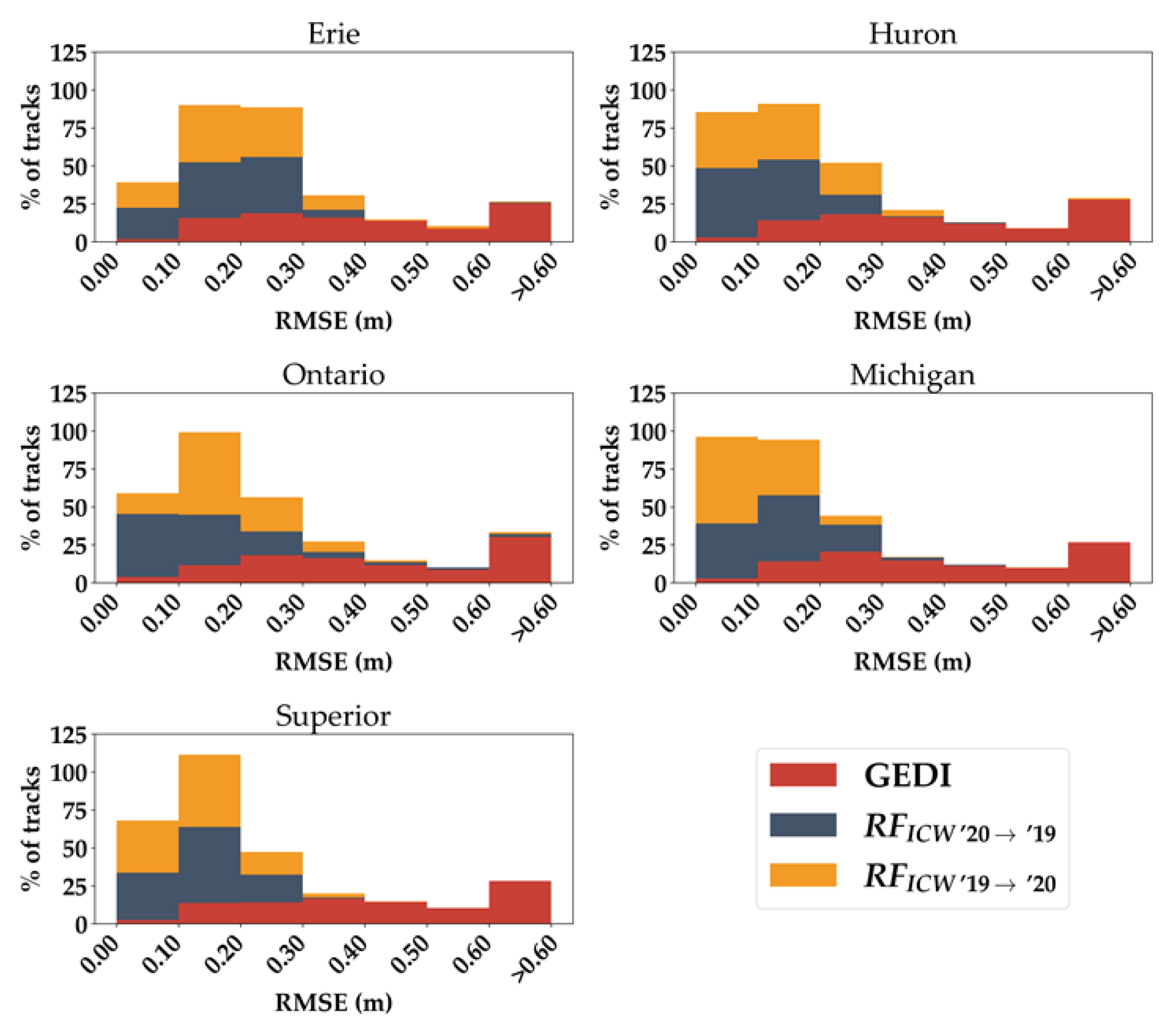
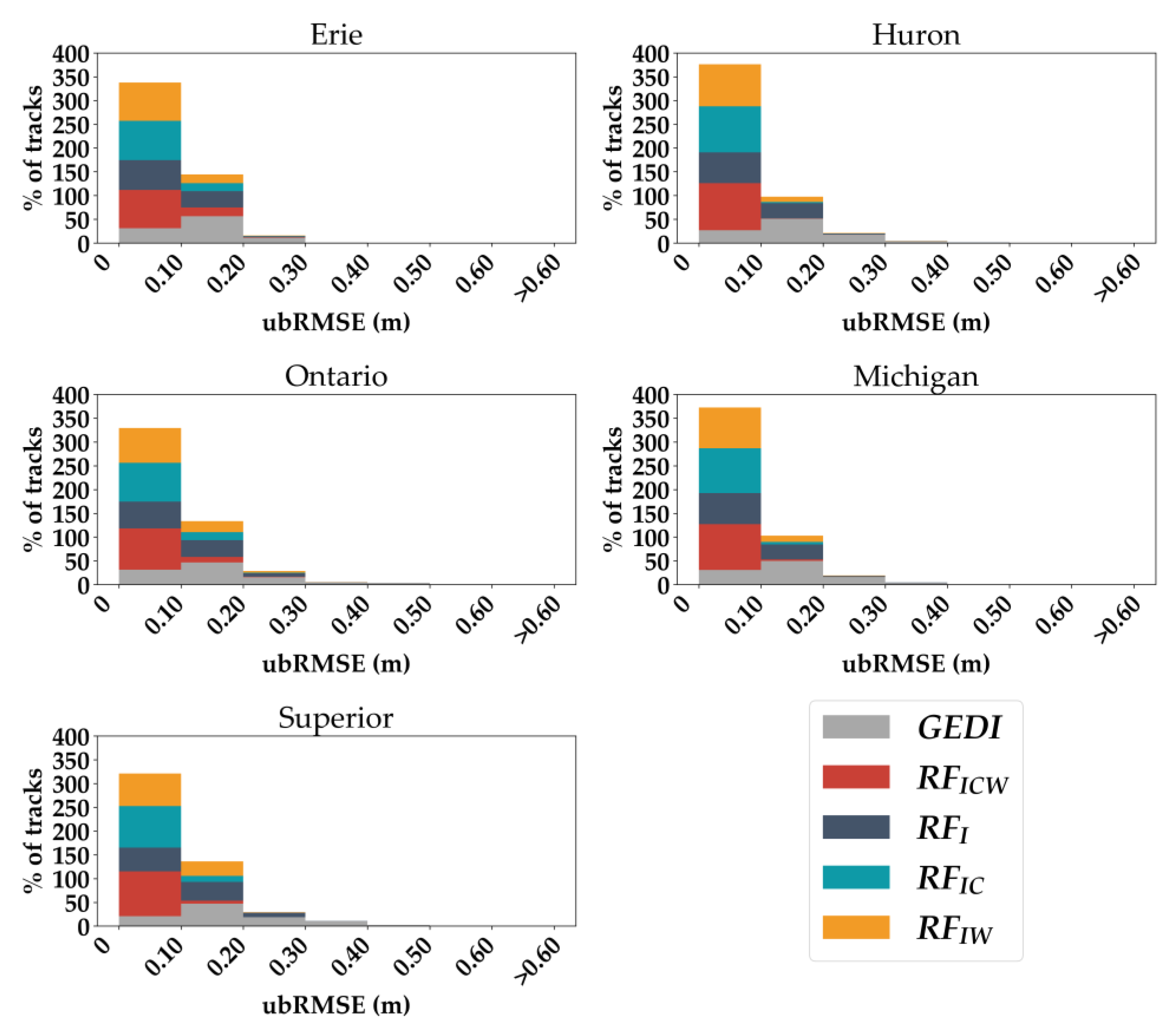
The proposed correction models that take instrumental, atmospheric, and wave surface variables into account in order to correct GEDI elevation estimates appear to greatly reduce uncertainties on these elevation estimates. Using the full model (based on instrumental, atmospheric, and wave surface: R F I C W ), fivefold cross-validated results showed an error (RMSE) on the estimation of water levels that ranged between 0.10 m and 0.14 m for lakes Erie, Huron, Michigan, and Superior, and 0.28 m for Lake Ontario. Moreover, the bias seemed to be mostly eliminated, with a bias ranging from −0.06 m (Lake Erie) to 0.01 m (Lake Superior). The proposed full model also generalizes well across the temporal and spatial domains. The temporal validation (training of model on a given year and validation on another year) of R F I C W shows errors (RMSE) on the retrieved water levels that ranged from 0.14 m (Lake Michigan) to 0.29 m (Lake Ontario), with a bias ranging from −0.07 m (Lake Erie) to 0.03 m (Lake Ontario).
Nonetheless, accounting for the fact that the tested full model showed an increase in accuracy by at least 92% with more than 74% of the variance explained, the remaining unexplained variance could be due to two factors. First, a large number of dependent variables were used for the modelling of GEDI elevation errors. However, given the complex interaction between LiDAR and the atmosphere and the water surface, not all the factors affecting the precision of LiDAR altimetry could be accounted for. Second, the available dependent variables used in this study were not error-free, because they were not direct measurements but resulted from models. For example, the accuracy on significant wave heights was around 10%, with a bias of less than 5%, or ~30 cm [24]. These two factors might explain some of the remaining uncertainty on the corrected GEDI elevation estimates.
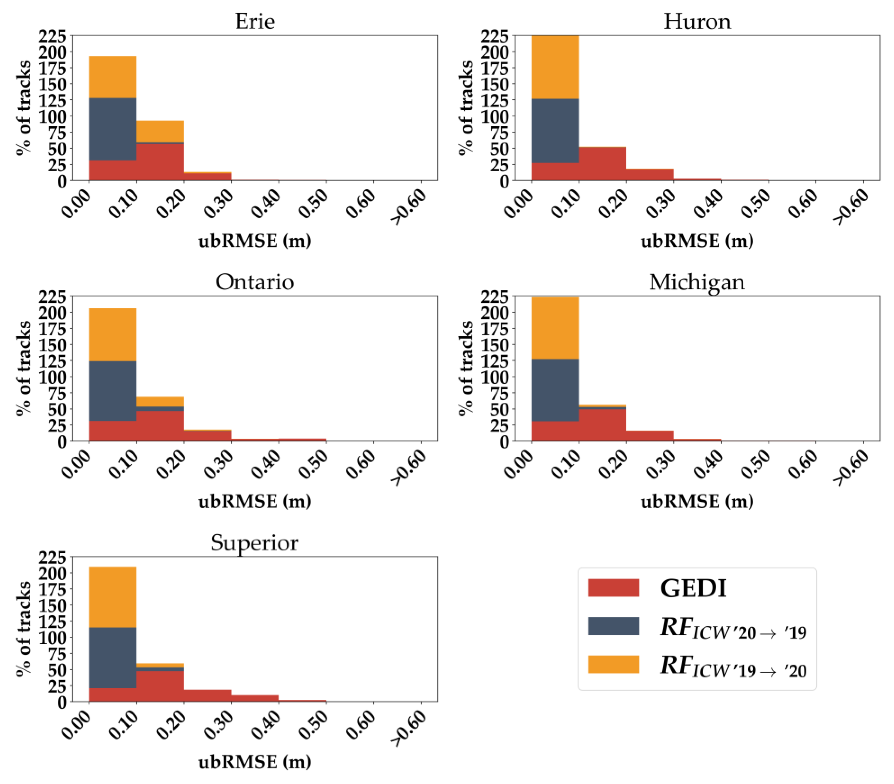
Regarding the spatial validation (training of model on a given lake and validation on another lakes), the uncertainty of GEDI’s corrected water level estimates differed based on the training and validation sites. Data over Lakes Michigan, Superior, and Huron were able to retrieve water levels well, with a mean RMSE ranging from 0.17 m ( R F I C W trained with Michigan data) to 0.19 m ( R F I C W trained with either Ontario or Superior data). Lakes Erie and Ontario showed lower generalization capabilities, with a mean RMSE of 0.26 m ( R F I C W trained with either Erie or Ontario data). Moreover, Lake Ontario was the lake where model generalization was the least accurate (corrected water level estimates using a model trained from other lakes), since the RMSE on water level estimates over Lake Ontario ranged from 0.21 m (model trained using Superior or Michigan data) to 0.24 m (model trained using Erie data).
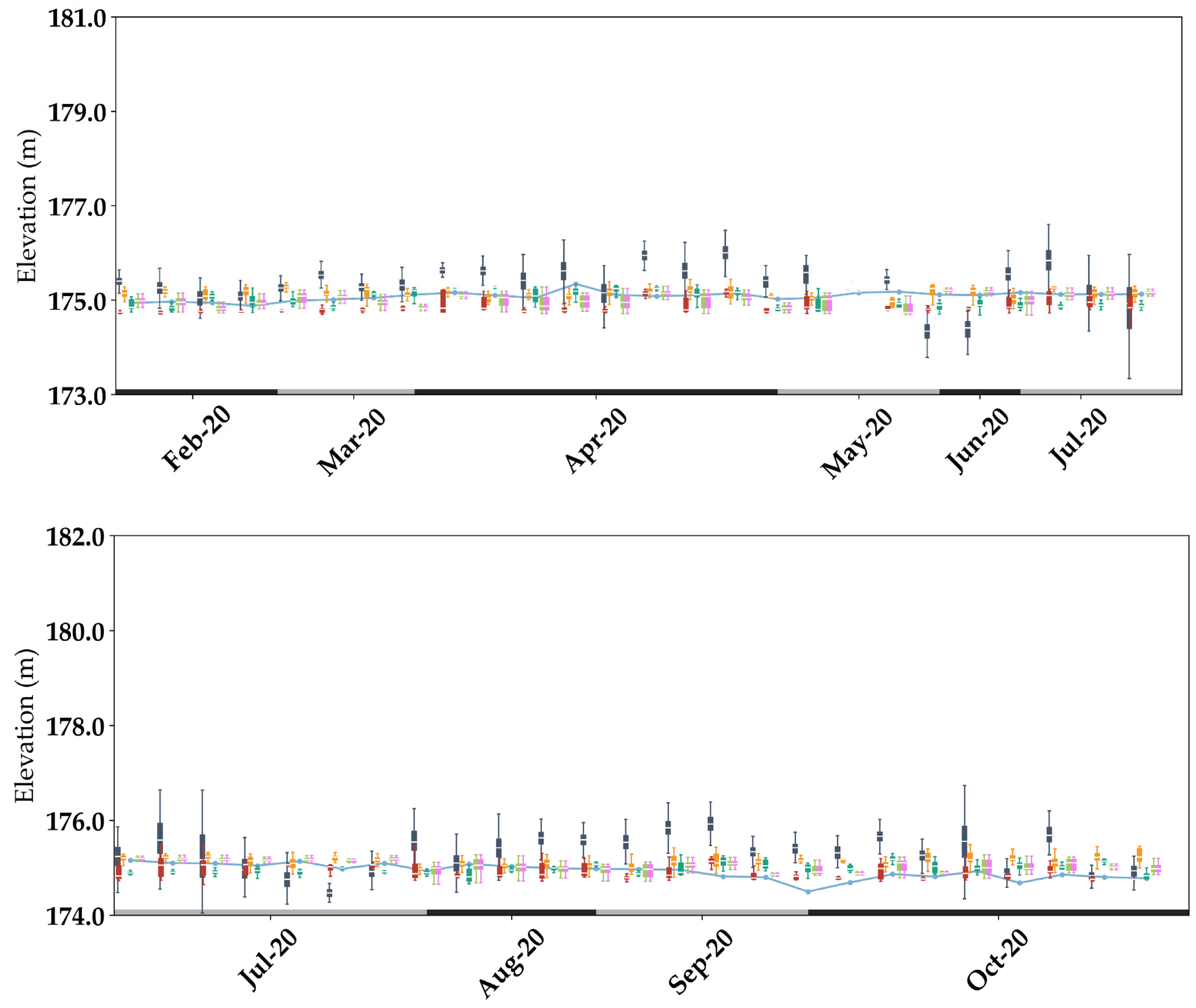
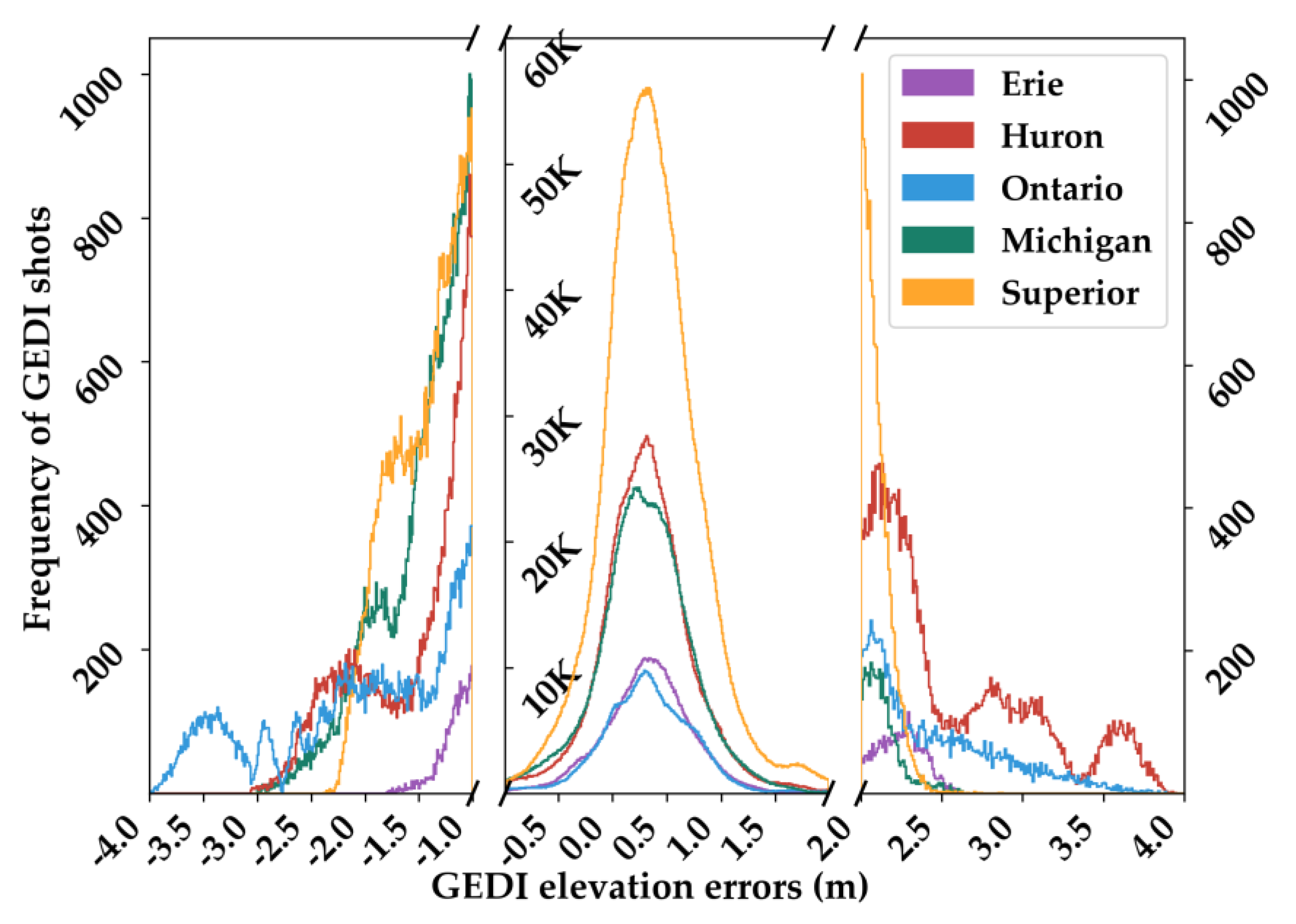
The generalization capabilities of the proposed full model ( R F I C W 
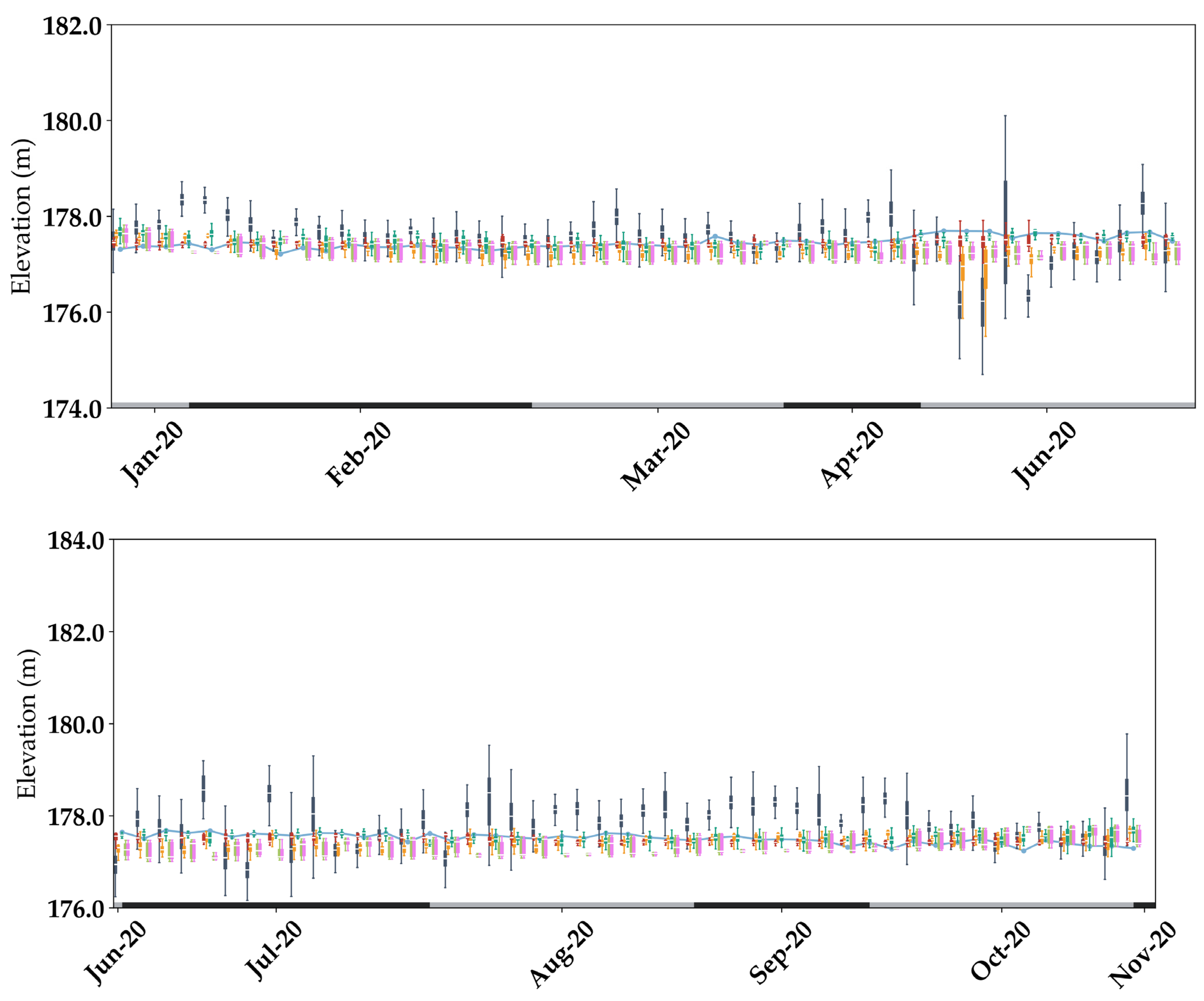
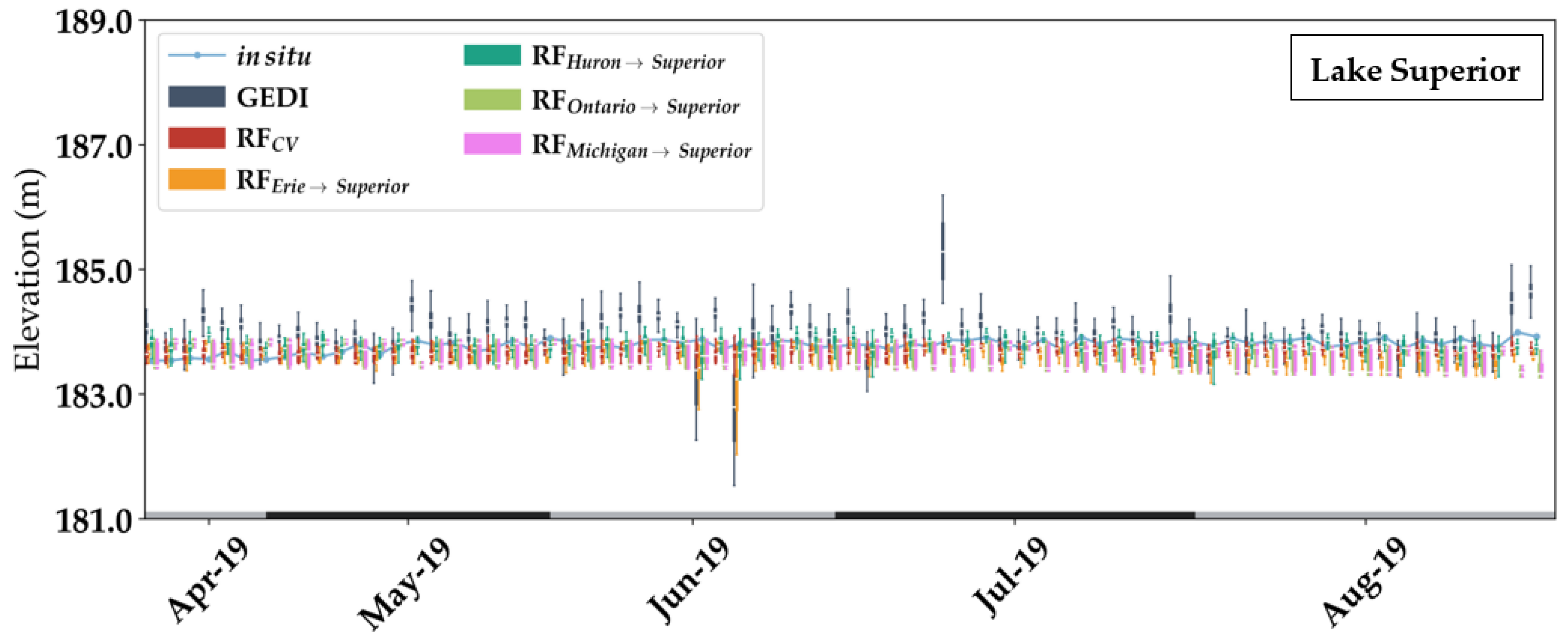
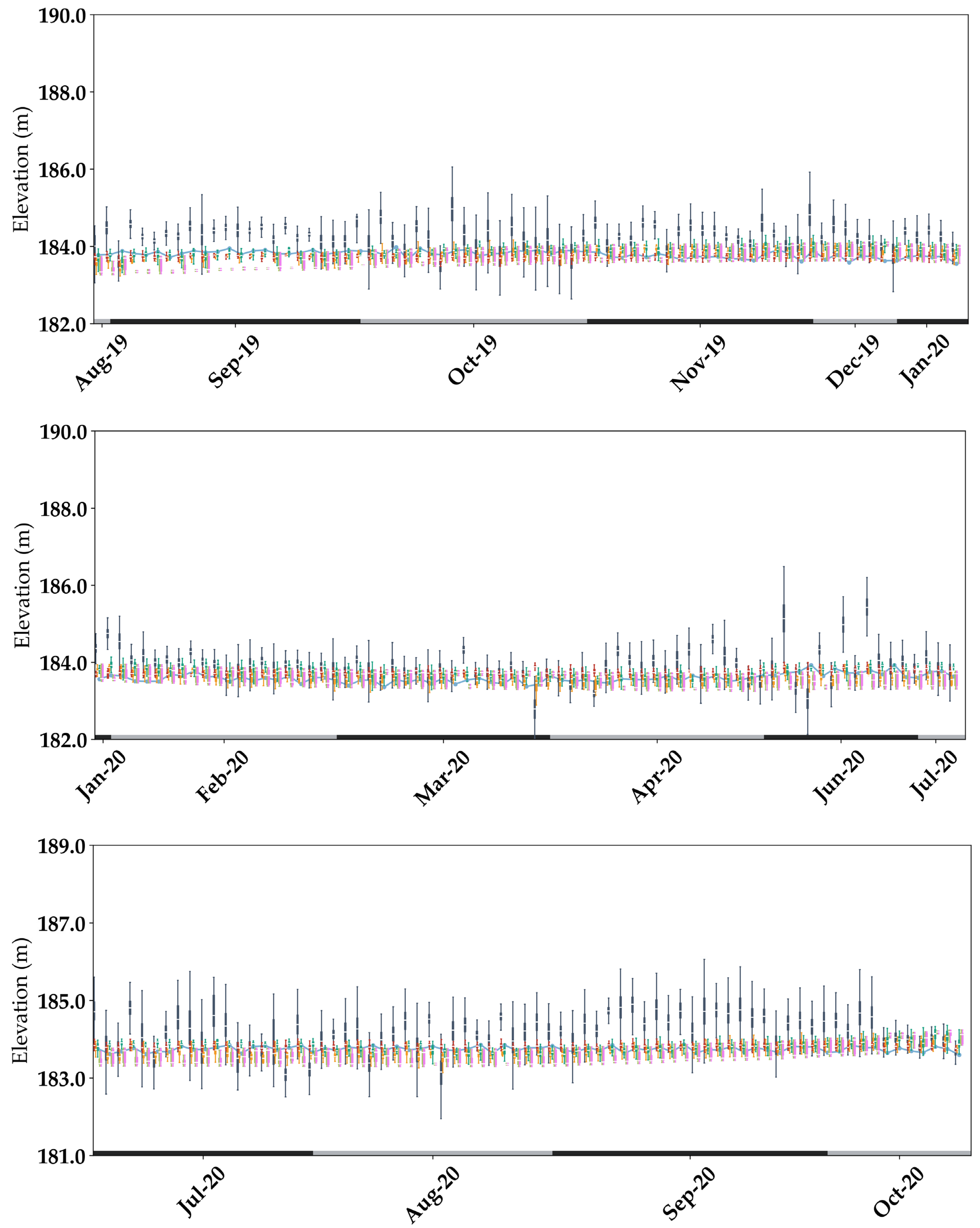
), either spatially or temporally, seems to be greatly affected by the number of GEDI acquisitions that the model was trained on. Indeed, the three most generalizable models were the models trained over Lake Superior (~4.84 M shots over 337 dates, Figure 13), Lake Huron (~2.25 M shots over 230 dates, Figure 13) and Lake Michigan (~2.16 M shots over 249 dates, Figure 13), whereas the models trained over Lakes Ontario and Erie showed less accurate results due to a smaller amount of training data (~0.88 M shots each, 113 dates over Lake Erie, and 116 over Lake Ontario, 
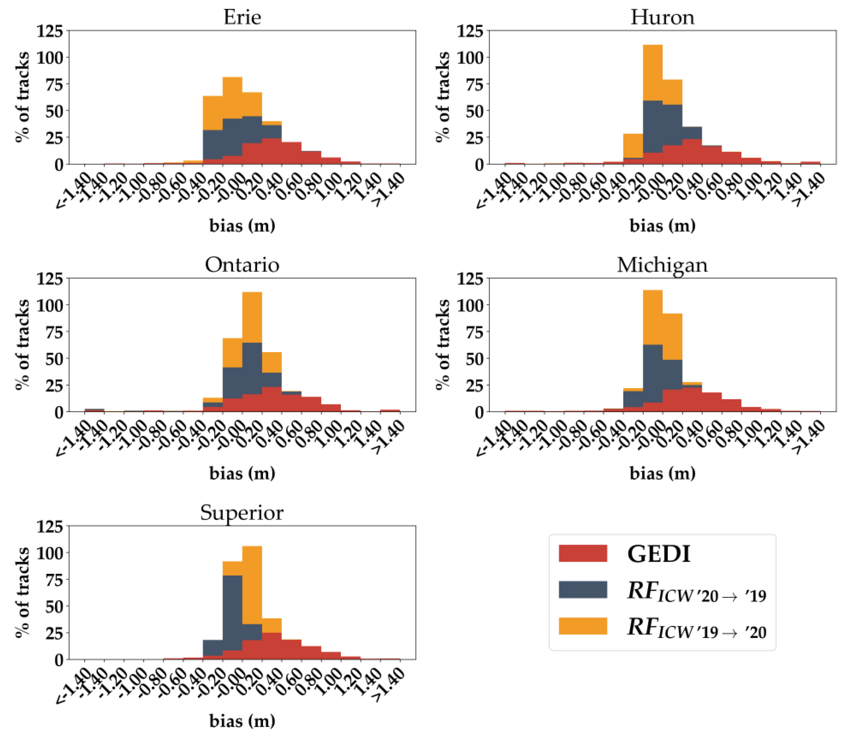
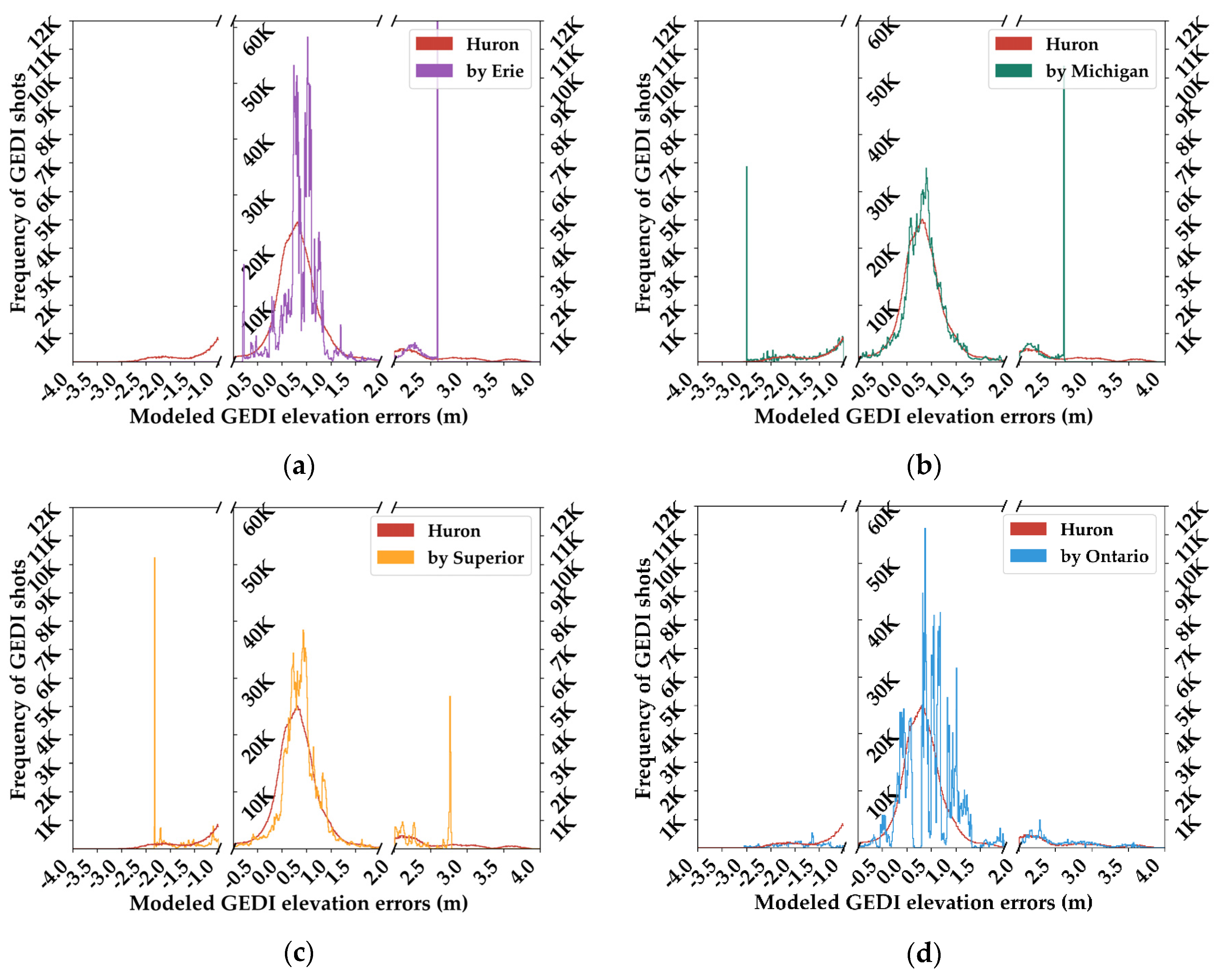
Figure 13). Indeed, by comparing the Jensen–Shannon divergence (JSD) between the original distribution of GEDI errors over Lake Huron and the distribution of modeled GEDI elevations errors obtained from models trained over Lakes Erie, Ontario, Michigan, and Superior (Figure 14), the modeled distribution with the least divergence was obtained from the model trained over Lake Michigan (JSD of 0.11), followed by the model trained over Lake Superior (JSD of 0.16). The distribution of GEDI elevation errors obtained from Lakes Erie and Ontario had the highest divergence to the original distribution of GEDI elevation errors with JSDs of, respectively, 0.29 and 0.37.
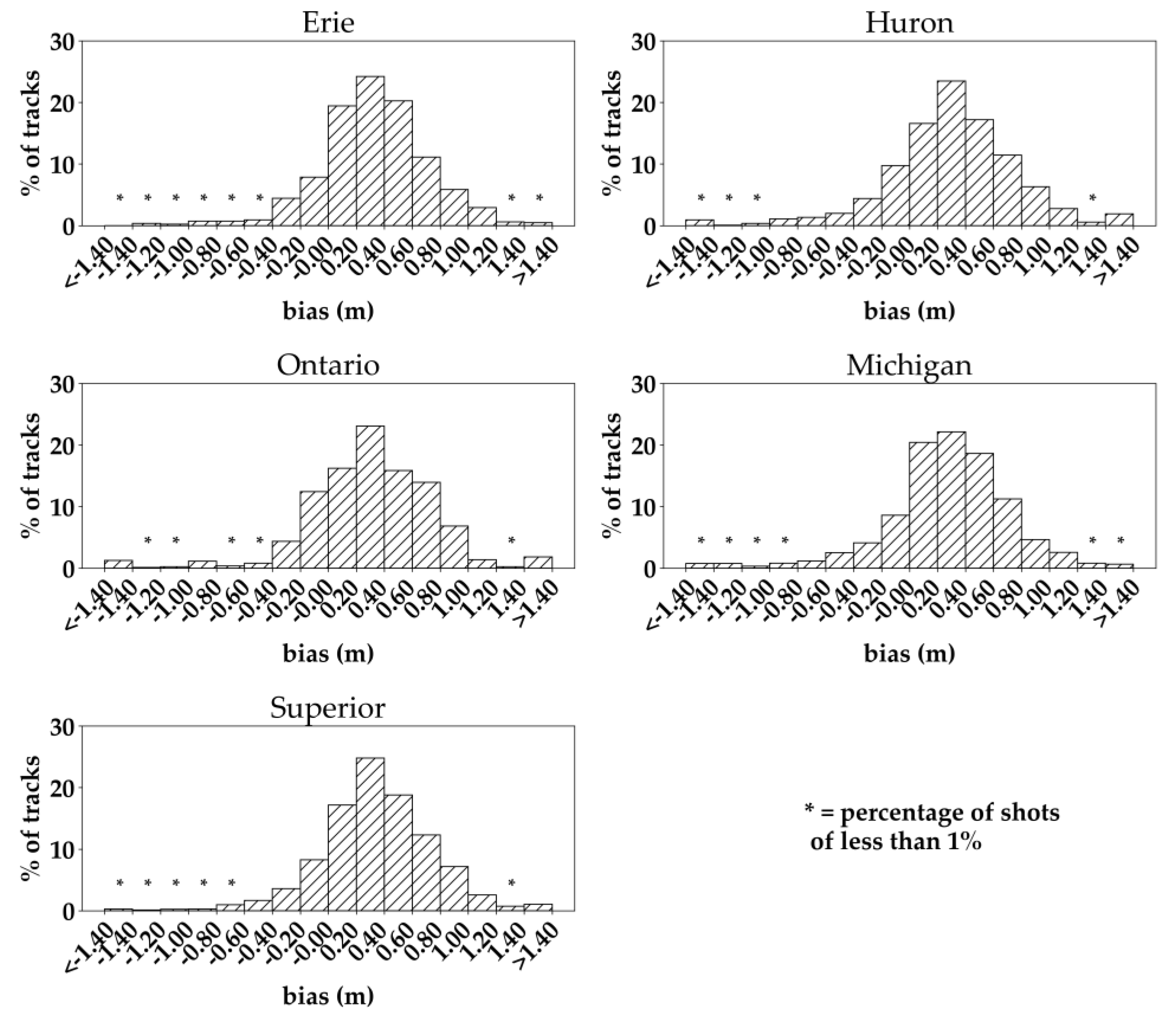
Although model generalizability seems correlated to the number of available acquisitions, since a higher number of training data increases the probability of the model being trained with shots acquired over different conditions, another factor that can have an influence on the accuracy of a generalization model is the range of distributions of GEDI elevation errors used for training. As such, a model trained over a given lake can only estimate the differences between GEDI and in situ water levels (i.e., errors) within its sampling distribution, leading to more uncertainties when correcting GEDI elevation estimates when the original differences between GEDI and in situ elevations are outside of this range. The effect of this factor can be seen in the distribution of modeled GEDI elevation errors in Figure 14. For example, the range of the distribution of GEDI elevation errors over Lake Huron extends from −3.1 m to 3.9 m (Figure 13), while a model trained using Lake Erie data can only estimate GEDI elevation errors from −0.4 m to 2.6 m (Figure 14a). This range (−0.4–2.6 m) corresponds to the range of the original distribution of errors over Lake Erie (Figure 13). Similarly, a model trained over Lake Michigan can only estimate errors within the range −3.0–2.6 m (Figure 14b), and −2.3–2.7 m for Lake Superior (Figure 14c). Conversely, a model trained over Lake Ontario, given its original distribution of GEDI elevation errors that extends from −4.0 to 4.0 m (Figure 13), can estimate errors within the full range of errors over Lake Huron (Figure 14d). This could also explain, for example, why the models trained over Lakes Huron, Ontario, Michigan, and Superior presented lower uncertainties in the estimation of the differences between GEDI and in situ elevations over Lake Erie, while a model trained over Lake Erie was less accurate when validated over the other four lakes.
The tested R F I C W model variants, while very spatially and temporally accurate, given the used set of variables, is practically infeasible over many other sites, as information on waves and other surface variables are hard to acquire. Indeed, the wave variables were obtained from NOAA’s Great Lakes waves’ model, that is based on the third-generation wave model, where data is only available over a selected number of lakes. Moreover, a significant number of lakes do not have significant waves. Therefore, from an operational standpoint, a model for the correction of GEDI elevation estimates using instrumental and atmospheric variables without water surface information is easier to train and deploy than a full model. In this study, the random forest models using instrumental only and instrumental and atmospheric variables showed high accuracy in the correction of GEDI’s elevation estimates. Moreover, while a model trained using only instrumental variables ( R F I ) was the least accurate, the obtained results with such a model improved the original GEDI elevation estimates by a factor of two. Regarding the R F I C model, only a small degradation in performance was observed in a comparison to the full model ( R F I C W 
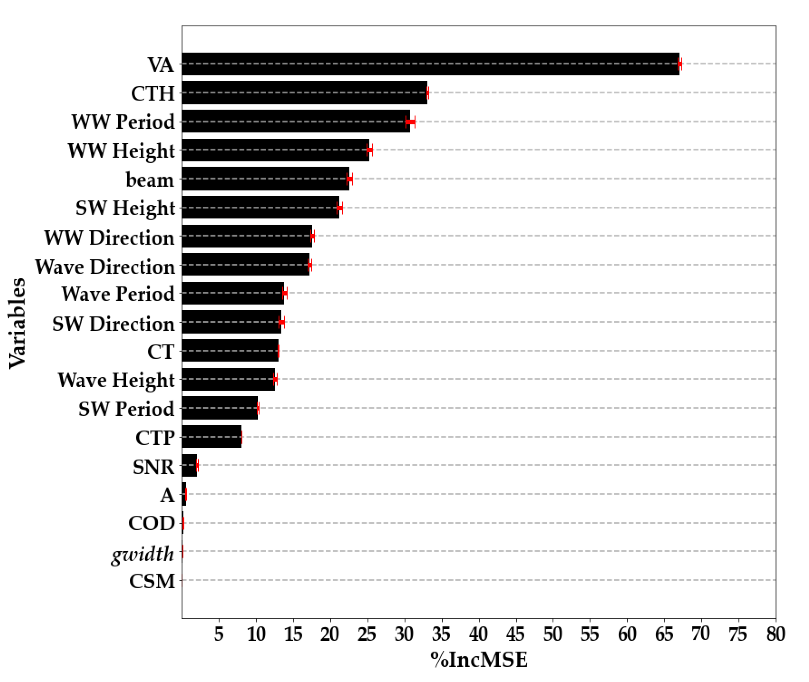
). Moreover, in this study, we used atmospheric data from the GOES-R satellites that only cover the American continent; globally, atmospheric data collected from other satellites can be used, such as the Meteosat Second Generation (MSG) series of satellites that cover Europe, Africa, and the Indian Ocean, and Himawari 8, that covers the Mid-Pacific. Quantitatively, to measure the effect of each variable on the accuracy of the model, a variable importance test was carried out. Variable importance is based on the mean decrease in the mean squared errors (MSE) and is measured as follows: first, the MSEf of the full model (model using all the variables from all the lakes) is calculated; next, the variable to calculate its importance is permuted through N iterations, and at each iteration, the model accuracy (MSEv) is calculated; finally, the variable importance is the difference between the MSEf and the average of the MSEv. The variable importance test showed that the group of variables with the highest effect (percentage increase in the mean square error of the regressions—%IncMSE) are the instrumental and atmospheric variables with a %IncMSE of, respectively, 46.2% and 45.8%. The %IncMSE of water surface state variables was 26.8%. Moreover, the %IncMSE of individual variables shows that the viewing angle (VA) was the most important variable, with an importance factor that is at least two times higher than the remaining input variables. Following VA is the cloud height (CTH), followed by the period of wind-generated waves. The cloud height and the height of wind-generated waves have almost the same importance. The variable importance of all the variables can be found in Figure A11.
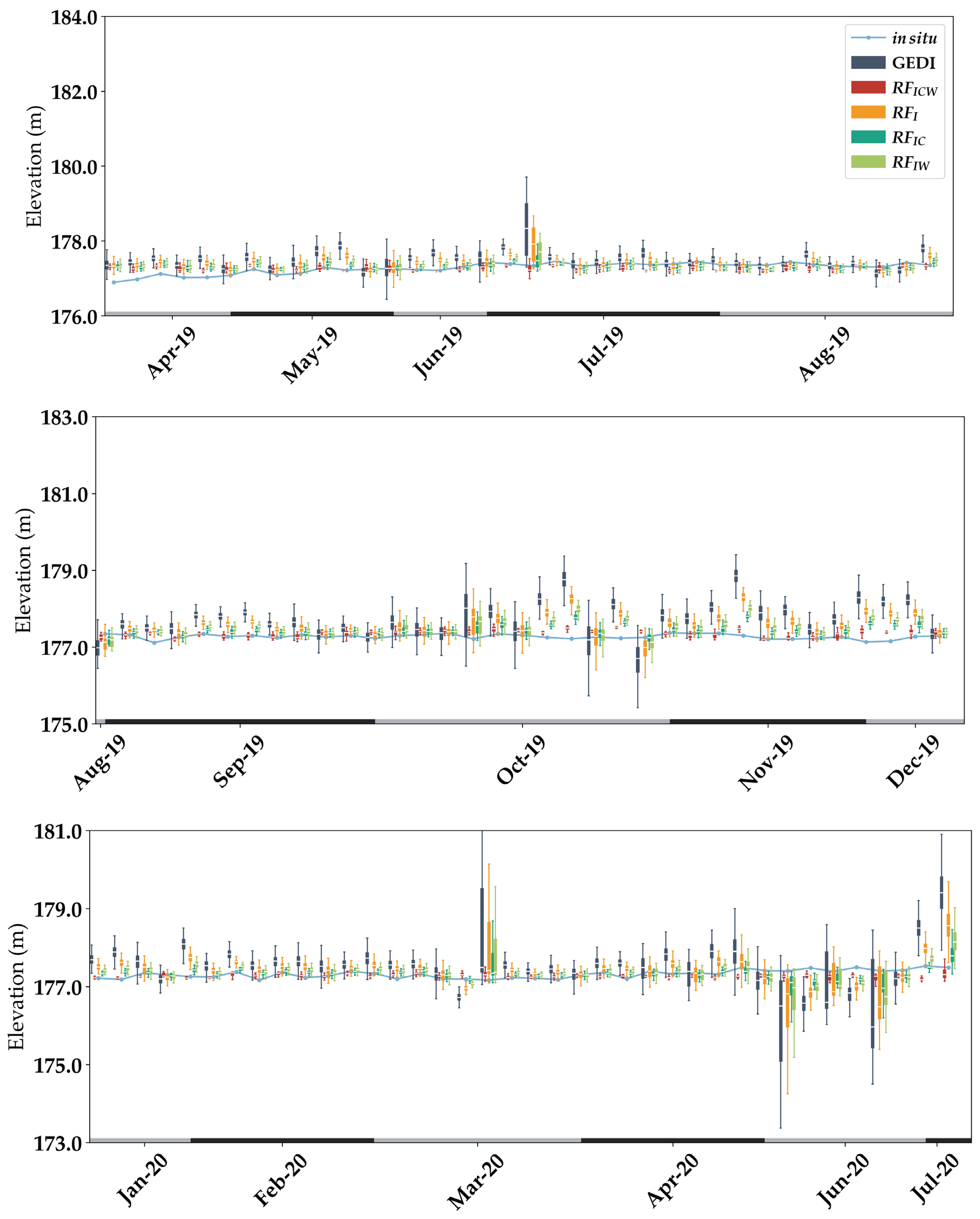
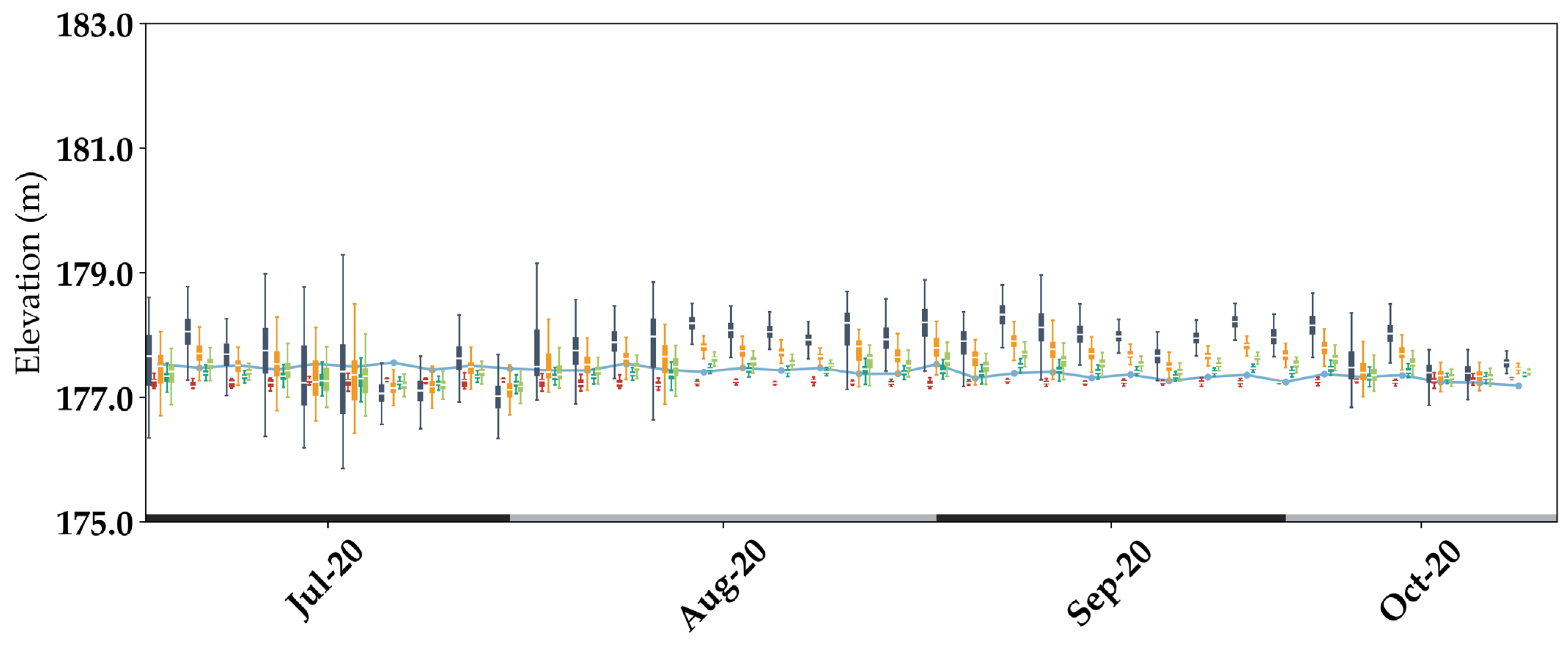
Finally, the proposed models in this article were developed to decrease the inaccuracy of GEDI elevation estimates at the footprint scale. As such, specific emphasis on uncertainties originating from in situ measurements and impacts of autocorrelation between successive GEDI shots were not take account. In addition, over a given lake on a given date, a high number of measurements from each track are acquired (mean of 2000 GEDI footprints by track in this study), whereas only a few sampling points over a lake’s surface could prove enough. Therefore, going forward, an aggregate of corrected GEDI elevation estimates from each track could be calculated to further decrease the inaccuracy of these estimates. Aggregation could simply be the result of averaging the elevations of corrected GEDI elevation estimates within each track, if elevation estimates are independent in space and time; in that case, elevation errors could be quantified using the standard deviation of the mean. Alternatively, in the presence of autocorrelation between successive GEDI shots, autocorrelation must be modeled and estimated using techniques such as block-kriging, with uncertainty at the lake scale being computed accordingly. The relevance of such an approach was developed in the study of Abdallah et al. [25].

6. Conclusions

Our analysis of the accuracy of the original GEDI water level estimates over the five Great Lakes, which showed uncertainties (RMSE) ranging from 0.54 to 0.68 m, confirms that GEDI elevation estimates are not accurate enough for them to be an additional source of information for the retrieval and monitoring of inland water levels. Therefore, modeling of the uncertainties to correct these elevation estimates is required in order to benefit from the extensive dataset acquired by GEDI over the Earth’s surface.
In this study, random-forest-based models were used in order to estimate the differences between the original GEDI elevation estimates and in situ measurements (i.e., errors). The proposed models used a combination of factors related to instrumental, atmospheric, and water surface state factors as inputs, as these factors could have an effect on the accuracy of GEDI acquisitions. The first proposed random forest regression model ( R F I C W ), which uses all of these factors, showed high accuracy on the estimation of the GEDI’s errors, thus greatly improving GEDI elevation estimates. Indeed, temporal validation of the model ( R F I C W ) trained on data from a given year and validated on data from another year showed an RMSE on the corrected elevation estimates (resp. R2) ranging between 0.14 and 0.24 m (R2 ranging between 0.70 and 0.92). Concerning the spatial validation ( R F I C W , trained over a lake and validated over the remaining four), the results varied based on the data of the lake used for training. For instance, the most accurate spatially validated model showed an RMSE that ranged between 0.16 and 0.21 m (R2 ranging between 0.86 and 0.93), while the least accurate model showed an RMSE that ranged between 0.16 and 0.29 m (R2 ranging between 0.63 and 0.85).
From an operational standpoint, the proposed full model was hard to train and deploy because it used factors of water surface states that are only available for a select few lakes worldwide. Therefore, three additional models with a reduced number of input factors were used. The first model used instrumental factors only, as they are always available, while the second model ( R F I C ) used atmospheric factors as well as instrumental factors, and the third model used water surface state factors ( R F I W ) in addition to instrumental factors. The results showed that, using only the instrumental factors, a correction with a factor of two could be obtained in comparison with the original GEDI elevation estimates. Regarding the two remaining models ( R F I C and R F I W ), they showed similar correction capabilities, with the R F I C model being slightly more accurate. Moreover, only a small degradation in the correction capabilities was observed with the R F I C model (RMSE ranged between 0.19 and 0.35 m, R2 ranged between 0.69 and 0.89) in comparison with the full model ( R F I C W ). Therefore, even in the absence of water surface state variables, our proposed methodology can be used in order to greatly reduce the uncertainty of GEDI elevation estimates globally.

Author Contributions

Conceptualization, I.F., N.B., J.-S.B. and F.F.; methodology, I.F., N.B. and J.-S.B.; software, I.F.; validation, I.F., N.B., J.-S.B., F.F. and N.P.R.; formal analysis, I.F., N.B., J.-S.B. and F.F.; data curation, I.F. and N.P.R.; writing—original draft preparation, I.F., N.B. and N.P.R.; writing—review and editing, J.-S.B. and F.F.; visualization, I.F. and N.P.R. All authors have read and agreed to the published version of the manuscript.

Funding

This research received funding from the French Space Study Center (CNES, TOSCA 2022 project) and the National Research Institute for Agriculture, Food, and the Environment (INRAE).

Data Availability Statement

Water levels were downloaded from NOAA’s Center for Operational Oceanographic Products and Services (CO-OPS) and the Fisheries and Oceans Department of Canada. Geostationary Operational Environmental Satellites data were downloaded from NOAA’s GOES on AWS. Water surface state factors were download from NOAA’s Environmental Modelling Center. Gedi data were downloaded from The Land Processes Distributed Active Archive Center.

Acknowledgments

The authors would like to thank the GEDI team and the NASA LPDAAC (Land Processes Distributed Active Archive Center) for providing GEDI data.

Conflicts of Interest

The authors declare no conflict of interest.

Appendix A

Figure A1. Bias (m) and ubRMSE (m) of GEDI acquisition time series across the five lakes. Each dot represents the bias or ubRMSE of multiple GEDI shots from the same track (i.e., shots acquired on the same date with the same beam).
Remotesensing 14 02361 g0a1

Appendix B

Figure A2. Box plot by track of the original estimated elevations by GEDI over Lake Erie and the four tested models presented in Section 3.1.1 and Section 3.1.2. The blue line represents in situ elevations.
Remotesensing 14 02361 g0a2aRemotesensing 14 02361 g0a2b
Figure A3. Boxplot by track of the original estimated elevations by GEDI over Lake Ontario and the four tested models presented in Section 3.1.1 and Section 3.1.2. The blue line represents in situ elevations.
Remotesensing 14 02361 g0a3aRemotesensing 14 02361 g0a3b
Figure A4. Boxplot by track of the original estimated elevations by GEDI over Lake Michigan and the four tested models presented in Section 3.1.1 and Section 3.1.2. The blue line represents in situ elevations.
Remotesensing 14 02361 g0a4aRemotesensing 14 02361 g0a4b
Figure A5. Boxplot by track of the original estimated elevations by GEDI over Lake Superior and the four tested models presented in Section 3.1.1 and Section 3.1.2. The blue line represents in situ elevations.
Remotesensing 14 02361 g0a5aRemotesensing 14 02361 g0a5b

Appendix C

Figure A6. Boxplot by track of the original estimated elevations by GEDI over Lake Erie and the five tested models presented in Section 3.1.3. The green line represents in situ elevations. R F C V represents the 5-fold cross-validation results over Lake Erie. R F H u r o n E r i e , R F O n t a r i o E r i e , R F M i c h i g a n E r i e , and R F S u p e r i o r E r i e represent the results of the models trained over Lakes Huron, Ontario, Michigan, and Superior, respectively, applied over Lake Erie.
Remotesensing 14 02361 g0a6aRemotesensing 14 02361 g0a6b
Figure A7. Boxplot by track of the original estimated elevations by GEDI over Lake Huron and the five tested models presented in Section 3.1.3. The green line represents in situ elevations. R F C V represents the 5-fold cross-validation results over Lake Huron. R F E r i e H u r o n , R F O n t a r i o H u r o n , R F M i c h i g a n H u r o n , and R F S u p e r i o r H u r o n represent the results of the models trained over Lakes Erie, Ontario, Michigan, and Superior, respectively, applied over Lake Huron.
Remotesensing 14 02361 g0a7aRemotesensing 14 02361 g0a7b
Figure A8. Boxplot by track of the original estimated elevations by GEDI over Lake Ontario and the five tested models presented in Section 3.1.3. The green line represents in situ elevations. R F C V represents the 5-fold cross-validation results over Lake Ontario. R F E r i e O n t a r i o , R F H u r o n O n t a r i o , R F M i c h i g a n O n t a r i o , and R F S u p e r i o r O n t a r i o represent the results of the models trained over Lakes Erie, Huron, Michigan, and Superior, respectively, applied over Lake Ontario.
Remotesensing 14 02361 g0a8aRemotesensing 14 02361 g0a8b
Figure A9. Boxplot by track of the original estimated elevations by GEDI over Lake Michigan and the five tested models presented in Section 3.1.3. The green line represents in situ elevations. R F C V represents the 5-fold cross-validation results over Lake Michigan. R F E r i e M i c h i g a n , R F H u r o n M i c h i g a n , R F O n t a r i o M i c h i g a n , and R F S u p e r i o r M i c h i g a n represent the results of the models trained over Lakes Erie, Huron, Ontario, and Superior, respectively, and applied over Lake Michigan.
Remotesensing 14 02361 g0a9aRemotesensing 14 02361 g0a9b
Figure A10. Boxplot by track of the original estimated elevations by GEDI over Lake Superior and the five tested models presented in Section 3.1.3. The green line represents in situ elevations. R F C V represents the 5-fold cross-validation results over Lake Superior. R F E r i e S u p e r i o r , R F H u r o n S u p e r i o r , R F O n t a r i o S u p e r i o r , and R F M i c h i g a n S u p e r i o r represent the results of the models trained over Lakes Erie, Huron, Ontario, and Michigan, respectively, and applied over Lake Superior.
Remotesensing 14 02361 g0a10aRemotesensing 14 02361 g0a10b

Appendix D

Figure A11. Variables’ order of importance in the error estimation random forest regression model with the percentage mean increase in MSE (%IncMSE) (higher values mean higher importance). WW represents wind generated waves variables. SW represents swell waves variables.
Remotesensing 14 02361 g0a11

References

  1. Younger, P.L. Water: All That Matters; Hodder & Stoughton: London, UK, 2015; ISBN 978-1-78539-007-4. [Google Scholar]
  2. Hannah, D.M.; Demuth, S.; van Lanen, H.A.J.; Looser, U.; Prudhomme, C.; Rees, G.; Stahl, K.; Tallaksen, L.M. Large-Scale River Flow Archives: Importance, Current Status and Future Needs. Hydrol. Process. 2011, 25, 1191–1200. [Google Scholar] [CrossRef]
  3. Shu, S.; Liu, H.; Beck, R.A.; Frappart, F.; Korhonen, J.; Lan, M.; Xu, M.; Yang, B.; Huang, Y. Evaluation of Historic and Operational Satellite Radar Altimetry Missions for Constructing Consistent Long-Term Lake Water Level Records. Hydrol. Earth Syst. Sci. 2021, 25, 1643–1670. [Google Scholar] [CrossRef]
  4. Frappart, F.; Calmant, S.; Cauhope, M.; Seyler, F.; Cazenave, A. Preliminary Results of ENVISAT RA-2-Derived Water Levels Validation over the Amazon Basin. Remote Sens. Environ. 2006, 100, 252–264. [Google Scholar] [CrossRef] [Green Version]
  5. Schwatke, C.; Dettmering, D.; Börgens, E.; Bosch, W. Potential of SARAL/AltiKa for Inland Water Applications. Mar. Geod. 2015, 38, 626–643. [Google Scholar] [CrossRef]
  6. Frappart, F.; Blarel, F.; Fayad, I.; Bergé-Nguyen, M.; Crétaux, J.-F.; Shu, S.; Schregenberger, J.; Baghdadi, N. Evaluation of the Performances of Radar and Lidar Altimetry Missions for Water Level Retrievals in Mountainous Environment: The Case of the Swiss Lakes. Remote Sens. 2021, 13, 2196. [Google Scholar] [CrossRef]
  7. Biancamaria, S.; Frappart, F.; Leleu, A.-S.; Marieu, V.; Blumstein, D.; Desjonquères, J.-D.; Boy, F.; Sottolichio, A.; Valle-Levinson, A. Satellite Radar Altimetry Water Elevations Performance over a 200 m Wide River: Evaluation over the Garonne River. Adv. Space Res. 2017, 59, 128–146. [Google Scholar] [CrossRef] [Green Version]
  8. Markus, T.; Neumann, T.; Martino, A.; Abdalati, W.; Brunt, K.; Csatho, B.; Farrell, S.; Fricker, H.; Gardner, A.; Harding, D.; et al. The Ice, Cloud, and Land Elevation Satellite-2 (ICESat-2): Science Requirements, Concept, and Implementation. Remote Sens. Environ. 2017, 190, 260–273. [Google Scholar] [CrossRef]
  9. Dubayah, R.; Blair, J.B.; Goetz, S.; Fatoyinbo, L.; Hansen, M.; Healey, S.; Hofton, M.; Hurtt, G.; Kellner, J.; Luthcke, S.; et al. The Global Ecosystem Dynamics Investigation: High-Resolution Laser Ranging of the Earth’s Forests and Topography. Sci. Remote Sens. 2020, 1, 100002. [Google Scholar] [CrossRef]
  10. Zhang, G.; Chen, W.; Xie, H. Tibetan Plateau’s Lake Level and Volume Changes From NASA’s ICESat/ICESat-2 and Landsat Missions. Geophys. Res. Lett. 2019, 46, 13107–13118. [Google Scholar] [CrossRef]
  11. Yuan, C.; Gong, P.; Bai, Y. Performance Assessment of ICESat-2 Laser Altimeter Data for Water-Level Measurement over Lakes and Reservoirs in China. Remote Sens. 2020, 12, 770. [Google Scholar] [CrossRef] [Green Version]
  12. Ryan, J.C.; Smith, L.C.; Cooley, S.W.; Pitcher, L.H.; Pavelsky, T.M. Global Characterization of Inland Water Reservoirs Using ICESat-2 Altimetry and Climate Reanalysis. Geophys. Res. Lett. 2020, 47, e2020GL088543. [Google Scholar] [CrossRef]
  13. Xiang, J.; Li, H.; Zhao, J.; Cai, X.; Li, P. Inland Water Level Measurement from Spaceborne Laser Altimetry: Validation and Comparison of Three Missions over the Great Lakes and Lower Mississippi River. J. Hydrol. 2021, 597, 126312. [Google Scholar] [CrossRef]
  14. Fayad, I.; Baghdadi, N.; Frappart, F. Comparative Analysis of GEDI’s Elevation Accuracy from the First and Second Data Product Releases over Inland Waterbodies. Remote Sens. 2022, 14, 340. [Google Scholar] [CrossRef]
  15. Urban, T.J.; Schutz, B.E.; Neuenschwander, A.L. A Survey of ICESat Coastal Altimetry Applications: Continental Coast, Open Ocean Island, and Inland River. Terr. Atmos. Ocean. Sci. 2008, 19, 1–19. [Google Scholar] [CrossRef] [Green Version]
  16. Baghdadi, N.N.; El Hajj, M.; Bailly, J.-S.; Fabre, F. Viability Statistics of GLAS/ICESat Data Acquired Over Tropical Forests. IEEE J. Sel. Top. Appl. Earth Obs. Remote Sens. 2014, 7, 1658–1664. [Google Scholar] [CrossRef] [Green Version]
  17. Fayad, I.; Baghdadi, N.; Riedi, J. Quality Assessment of Acquired GEDI Waveforms: Case Study over France, Tunisia and French Guiana. Remote Sens. 2021, 13, 3144. [Google Scholar] [CrossRef]
  18. Fayad, I.; Baghdadi, N.; Bailly, J.S.; Frappart, F.; Zribi, M. Analysis of GEDI Elevation Data Accuracy for Inland Waterbodies Altimetry. Remote Sens. 2020, 12, 2714. [Google Scholar] [CrossRef]
  19. Abshire, J.; Gardner, C. Atmospheric Refractivity Corrections in Satellite Laser Ranging. IEEE Trans. Geosci. Remote Sens. 1985, GE-23, 414–425. [Google Scholar] [CrossRef]
  20. Palm, S.P.; Yang, Y.; Herzfeld, U.; Hancock, D.; Hayes, A.; Selmer, P.; Hart, W.; Hlavka, D. ICESat-2 Atmospheric Channel Description, Data Processing and First Results. Earth Space Sci. 2021, 8, e2020EA001470. [Google Scholar] [CrossRef]
  21. Leys, C.; Ley, C.; Klein, O.; Bernard, P.; Licata, L. Detecting Outliers: Do Not Use Standard Deviation around the Mean, Use Absolute Deviation around the Median. J. Exp. Soc. Psychol. 2013, 49, 764–766. [Google Scholar] [CrossRef] [Green Version]
  22. Schmit, T.J.; Griffith, P.; Gunshor, M.M.; Daniels, J.M.; Goodman, S.J.; Lebair, W.J. A Closer Look at the ABI on the GOES-R Series. Bull. Am. Meteorol. Soc. 2017, 98, 681–698. [Google Scholar] [CrossRef]
  23. Breiman, L. Random Forests. Mach. Learn. 2001, 45, 5–32. [Google Scholar] [CrossRef] [Green Version]
  24. Stopa, J.E.; Ardhuin, F.; Babanin, A.; Zieger, S. Comparison and Validation of Physical Wave Parameterizations in Spectral Wave Models. Ocean Model. 2016, 103, 2–17. [Google Scholar] [CrossRef] [Green Version]
  25. Abdallah, H.; Bailly, J.-S.; Baghdadi, N.; Lemarquand, N. Improving the Assessment of ICESat Water Altimetry Accuracy Accounting for Autocorrelation. ISPRS J. Photogramm. Remote Sens. 2011, 66, 833–844. [Google Scholar] [CrossRef] [Green Version]
Figure 1. North American Great Lakes Region. The blue lines correspond to the GEDI acquisitions considered in this study.
Remotesensing 14 02361 g001
Figure 2. Example of the gauge stations over Lake Erie considered for the analysis of the accuracy of the GEDI track of the 31 October 2019 (beam 7).
Remotesensing 14 02361 g002
Figure 3. Mean absolute differences of the in situ water level measurements as a function of the distance of the gauge stations (by pairs).
Remotesensing 14 02361 g003
Figure 4. Distribution of the mean difference (bias) between GEDI shots and in situ elevations across the five studied lakes. Biases correspond to the mean difference calculated for a given track (GEDI shots acquired on a given date with a given beam).
Remotesensing 14 02361 g004
Figure 5. Distribution of the unbiased root mean squared error (ubRMSE) between GEDI shots and in situ elevations across the five studied lakes. The distribution corresponds to the ubRMSE of GEDI tracks (i.e., shots acquired on the same date with the same beam).
Remotesensing 14 02361 g005
Figure 6. Distribution of the root mean squared error (RMSE) between GEDI shots and in situ elevations across the five studied lakes. The distribution corresponds to the RMSE of GEDI tracks (i.e., shots acquired on the same date with the same beam).
Remotesensing 14 02361 g006
Figure 7. Boxplot by track of the original estimated elevations by GEDI over Lake Huron and the four tested models presented in Section 3.1.1 and Section 3.1.2. The blue line represents in situ elevations.
Remotesensing 14 02361 g007aRemotesensing 14 02361 g007b
Figure 8. Stacked histograms of the distribution of the mean difference (bias) between GEDI (resp. R F I C W   19 20 and R F I C W   20 19 ) and in situ elevations across the five studied lakes. Biases correspond to the mean difference calculated for GEDI shots grouped by acquisition date and the acquiring beam. R F I C W   19 20 (resp. R F I C W   20 19 ) corresponds to the R F I C W model, trained over 2019 (resp. 2020) data and validated on 2020 data (resp. 2019).
Remotesensing 14 02361 g008
Figure 9. Stacked histograms of the distribution of the unbiased root mean squared error (ubRMSE) between GEDI (resp.   R F I C W   19 20 and R F I C W   20 19 ) and in situ elevations across the five studied lakes. The distribution corresponds to the ubRMSE of GEDI shots grouped by acquisition date and the acquiring beam. R F I C W   19 20 (resp. R F I C W   20 19 ) corresponds to the R F I C W model, trained over 2019 (resp. 2020) data and validated on 2020 data (resp. 2019).
Remotesensing 14 02361 g009
Figure 10. Stacked histograms of the distribution of the root mean squared error (RMSE) between GEDI (resp. R F I C W   19 20 and R F I C W   20 19 ) and in situ elevations across the five studied lakes. The distribution corresponds to the RMSE of GEDI shots grouped by acquisition date and the acquiring beam. R F I C W   19 20 (resp. R F I C W   20 19 ) corresponds to the R F I C W model, trained over 2019 (resp. 2020) data and validated on 2020 data (resp. 2019).
Remotesensing 14 02361 g010
Figure 11. Stacked histograms of the distribution of the mean difference (bias) between GEDI (resp. R F I C W ,   R F I , R F I C , and R F I W ) and in situ elevations across the five studied lakes. Biases correspond to the mean difference calculated for GEDI shots grouped by acquisition date and the acquiring beam.
Remotesensing 14 02361 g011
Figure 12. Stacked histograms of the distribution of the unbiased root mean squared error (ubRMSE) between GEDI (resp. R F I C W ,   R F I , R F I C , and R F I W ) and in situ elevations across the five studied lakes. The distribution corresponds to the ubRMSE of GEDI shots grouped by acquisition date and the acquiring beam.
Remotesensing 14 02361 g012
Figure 13. Distribution of GEDI elevation errors across the five studied lakes.
Remotesensing 14 02361 g013
Figure 14. Distribution of the modeled GEDI elevation errors over Lake Huron (red histogram) after the application of the R F I C W model trained over Lake Erie (a), Michigan (b), Superior (c), and Ontario (d).
Remotesensing 14 02361 g014
Table 1. Global Ecosystem Dynamics Investigation (GEDI) acquisition dates between April 2019 and October 2020 and available GEDI shots count over the studied lakes.
GEDI Acquisition Dates CountGEDI Shots CountAverage Water Level (April 2019 through October 2020)Approximate Size (km2)
Lake Superior3376,358,428183.718 m82,100
Lake Michigan2492,753,218177.291 m57,800
Lake Huron2303,000,920177.139 m59,600
Lake Erie1131,102,068174.877 m25,670
Lake Ontario1161,062,20075.302 m19,010
Table 2. Summary of the three groups of factors used in this study for the correction of GEDI elevation estimates.
Variables GroupSourceVariables
Instrumental (I)GEDI
  • Water surface peak amplitude (A)
  • Water surface peak width (gwidth)
  • Viewing angle (VA)
  • Signal to noise ratio (SNR)
  • Acquiring beam (beam)
Cloud and atmospheric (C)GOES-R
  • Cleary sky mask (CSM)
  • Cloud type (CT)
  • Cloud top temperatures (CTT)
  • Cloud top heights (CTH)
  • Cloud optical depth (COD)
Water surface state (W)Great Lakes wave model (GLWU)
  • Information on swell waves: Includes three variables—height, period, and direction
  • Information on wind generated waves: Includes three variables—height, period, and direction
  • Information on wind: Includes two variables—direction and speed
  • Information on gusts: Includes two variables—direction and speed
  • Water surface temperature
  • Current direction
Table 3. Summary of the models and input variables that are tested in this study.
Model IDData UsedValidation StrategySection Reference
R F I C W I, C, and WTrained on 2019 acquisitions and validated over 2020 acquisitions and vice versa: lake by lakeSection 3.1.1
R F I ITrained on 2019 acquisitions and validated over 2020 acquisitions and vice versa: lake by lakeSection 3.1.2
R F I C I and CTrained on 2019 acquisitions and validated over 2020 acquisitions and vice versa: lake by lakeSection 3.1.2
R F I W I and WTrained on 2019 acquisitions and validated over 2020 acquisitions and vice versa: lake by lakeSection 3.1.2
R F i j
Where i is the lake used for training and j the lake used for validation
I, C, and WTraining on one lake and validating on anotherSection 3.1.3
Table 4. Summary statistics of the RMSE and ubRMSE on the estimation of water surface elevations from the original GEDI estimates, and the four tested models presented in Section 3.1.1 and Section 3.1.2.
RMSE (m)ubRMSE (m)Error Budget Explained Variance R2
LakeUE * R F I C W R F I R F I W R F I C UE * R F I C W R F I R F I W R F I C R F I C W R F I R F I W R F I C
Erie0.570.210.350.260.240.440.190.310.250.210.780.370.640.76
Huron0.660.180.410.300.220.590.180.380.290.220.910.500.740.86
Ontario0.680.240.450.380.350.610.290.450.380.340.740.490.670.70
Michigan0.640.140.350.260.190.520.130.320.230.170.920.540.780.89
Superior0.570.150.360.260.210.460.160.290.220.170.860.390.680.82
UE * represents the uncorrected GEDI water level estimates.
Table 5. Summary statistics of the bias on the estimation of water surface elevations using a random forest model trained using I, C, and W variables over a lake and applied to the remaining four. The diagonal line represents the results of the 5-fold cross-validation.
Training
ErieHuronOntarioMichiganSuperior
ValidationErie−0.06−0.100.050.040.03
Huron0.110.010.160.020.07
Ontario0.00−0.15−0.04−0.04−0.03
Michigan0.12−0.030.160.00−0.01
Superior0.07−0.070.11−0.010.01
Table 6. Summary statistics of the ubRMSE on the estimation of water surface elevations using a random forest model trained using I, C, and W variables over a lake and applied to the remaining four. The diagonal line represents the results of the 5-fold cross-validation.
Training
ErieHuronOntarioMichiganSuperior
ValidationErie0.120.140.160.160.16
Huron0.260.120.250.160.19
Ontario0.290.190.270.200.18
Michigan0.210.150.240.110.15
Superior0.190.170.250.170.10
Table 7. Summary statistics of the RMSE on the estimation of water surface elevations using a random forest models trained using I, C, and W variables over a lake and applied to the remaining four. The diagonal line represents the results of the 5-fold cross-validation.
Training
ErieHuronOntarioMichiganSuperior
ValidationErie0.140.170.160.160.16
Huron0.290.120.290.160.21
Ontario0.280.240.280.210.21
Michigan0.250.150.290.110.16
Superior0.200.180.280.160.10
Table 8. Summary statistics of the coefficient of determination (R2) on the estimation of the difference between GEDI and in situ water levels using a random forest model trained using I, C, and W variables over a lake and applied to the remaining four. The diagonal line represents the results of the 5-fold cross-validation.
Training
ErieHuronOntarioMichiganSuperior
ValidationErie0.880.840.850.860.86
Huron0.760.940.750.930.88
Ontario0.780.850.820.880.91
Michigan0.770.910.690.930.91
Superior0.800.840.630.870.93
Publisher’s Note: MDPI stays neutral with regard to jurisdictional claims in published maps and institutional affiliations.

