
RETRACTED: Geometric Construction of Video Stereo Grid Space
Abstract
:
1. Introduction
2. Related Work

| Calibration Method | Traditional Camera Calibration | Active-Vision Calibration | Camera Self-Calibration |
|---|---|---|---|
| Advantage | In the case of more accurate calibration objects, a higher accuracy can be obtained | The algorithm is more stable and robust | High flexibility and wide range of applications |
| Disadvantage | The calculation is relatively complicated | High requirements for equipment and limited application scope | Low precision |
3. Materials and Methods
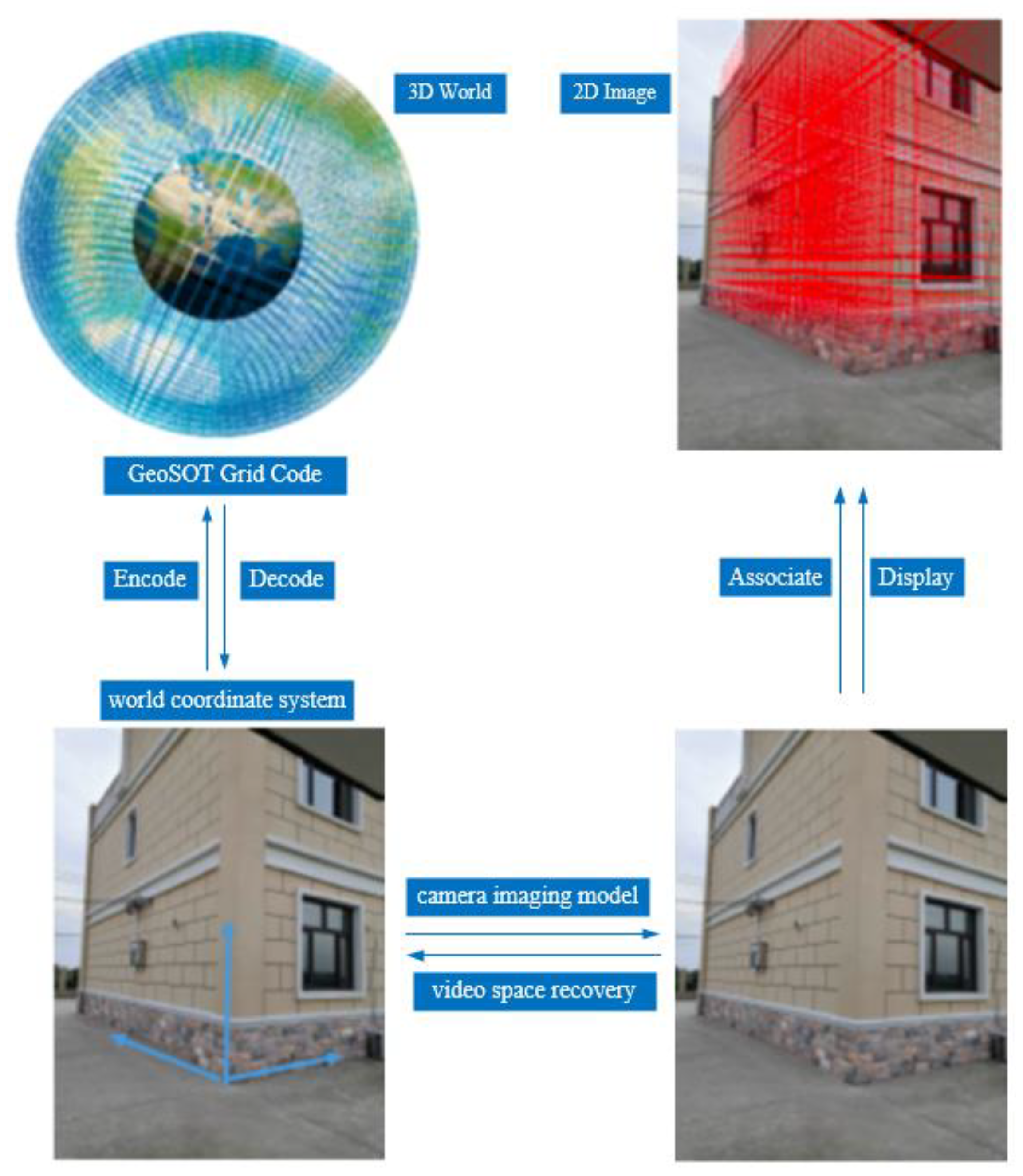
3.1. Model Architecture
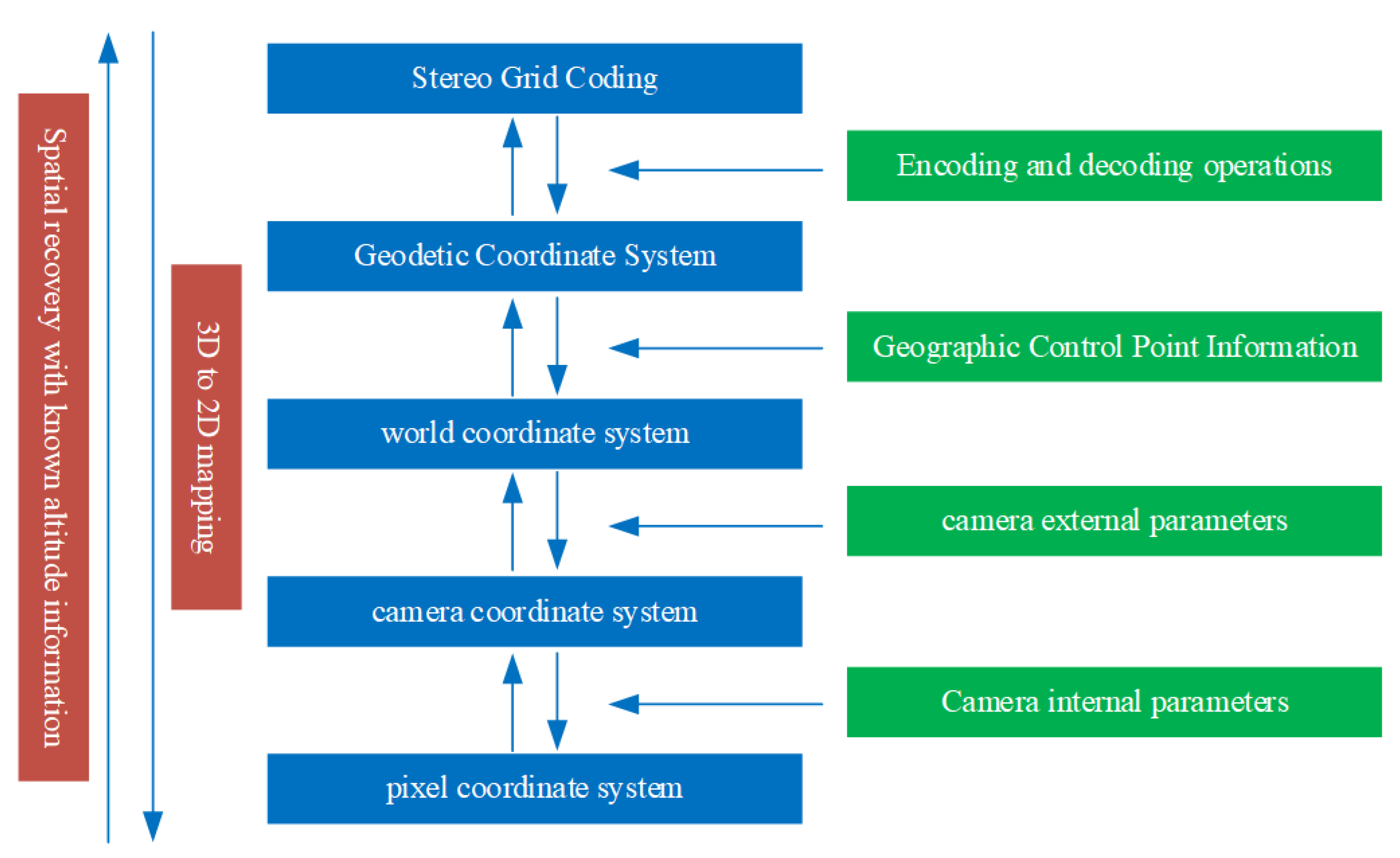
- Using the vanishing-point-based stereo space recovery optimization algorithm to clarify the camera parameters, the external parameters were used to determine the rotation angle and translation vector of the camera in the three-dimensional world. The inverse calculation of the camera imaging model could obtain the mapping of the 2D video frame to the 3D world coordinate system by solving the mapping from the camera world coordinate system to the camera coordinate system, and then using the internal parameters to determine the camera coordinate system in relation to the projection method of the 2D image.
- Based on the known geographic control points and other information, we first established a mapping relationship between the world coordinate system and the latitude and longitude geodetic coordinate system through the angle and scale solution information. Secondly, we passed the GeoSO-3D grid code to the geodetic coordinate system of latitude, longitude, and height, creating an encoding and decoding conversion relationship to realize the mapping relationship between the GeoSOT-3D grid code and the world coordinate system coordinates.
- The model completed the mapping of the known 3D height information from the 2D pixel coordinates to the three-dimensional grid code.
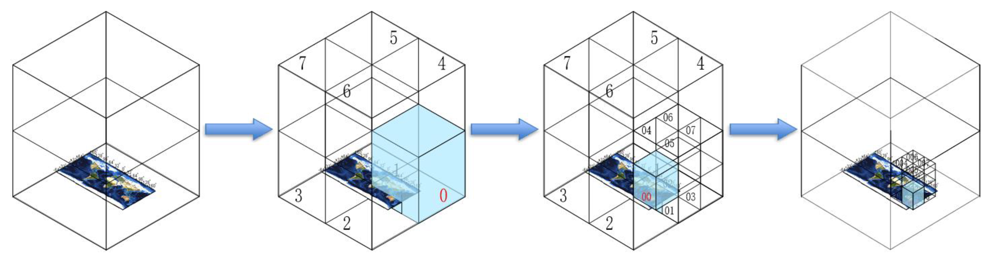
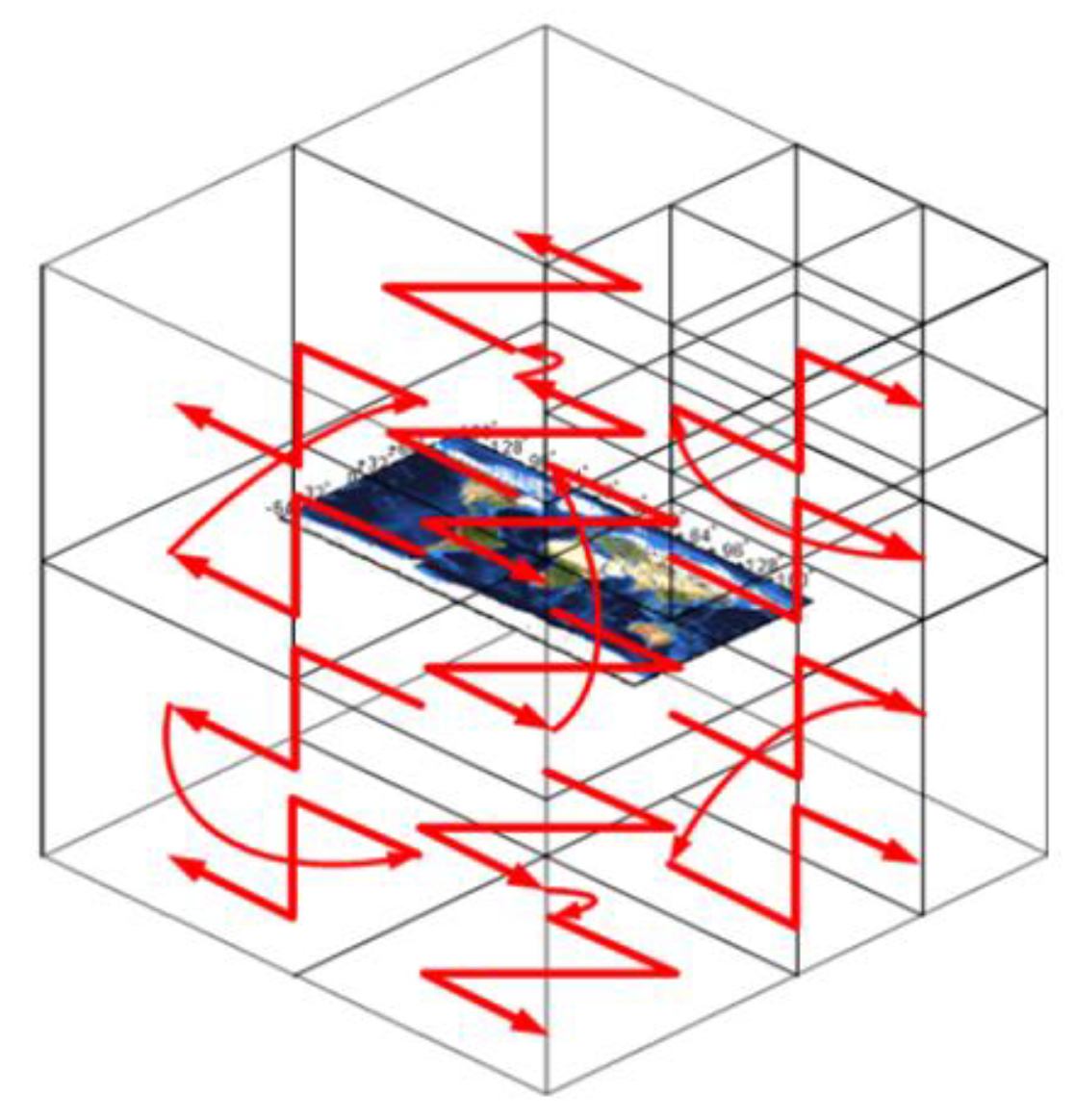
3.1.1. GeoSOT-3D Global Mesh Model
3.1.2. Camera Imaging Model
- 1.
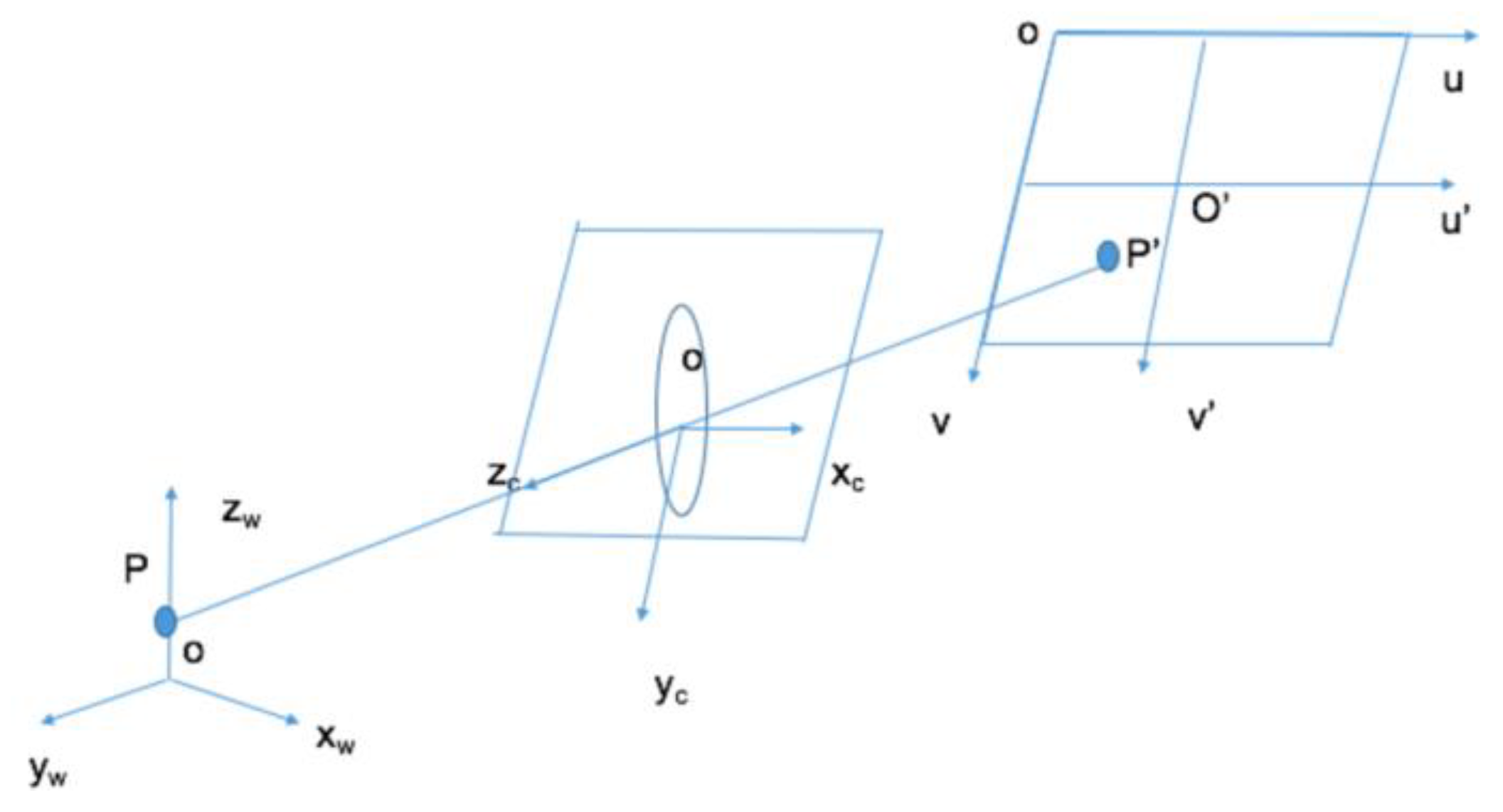
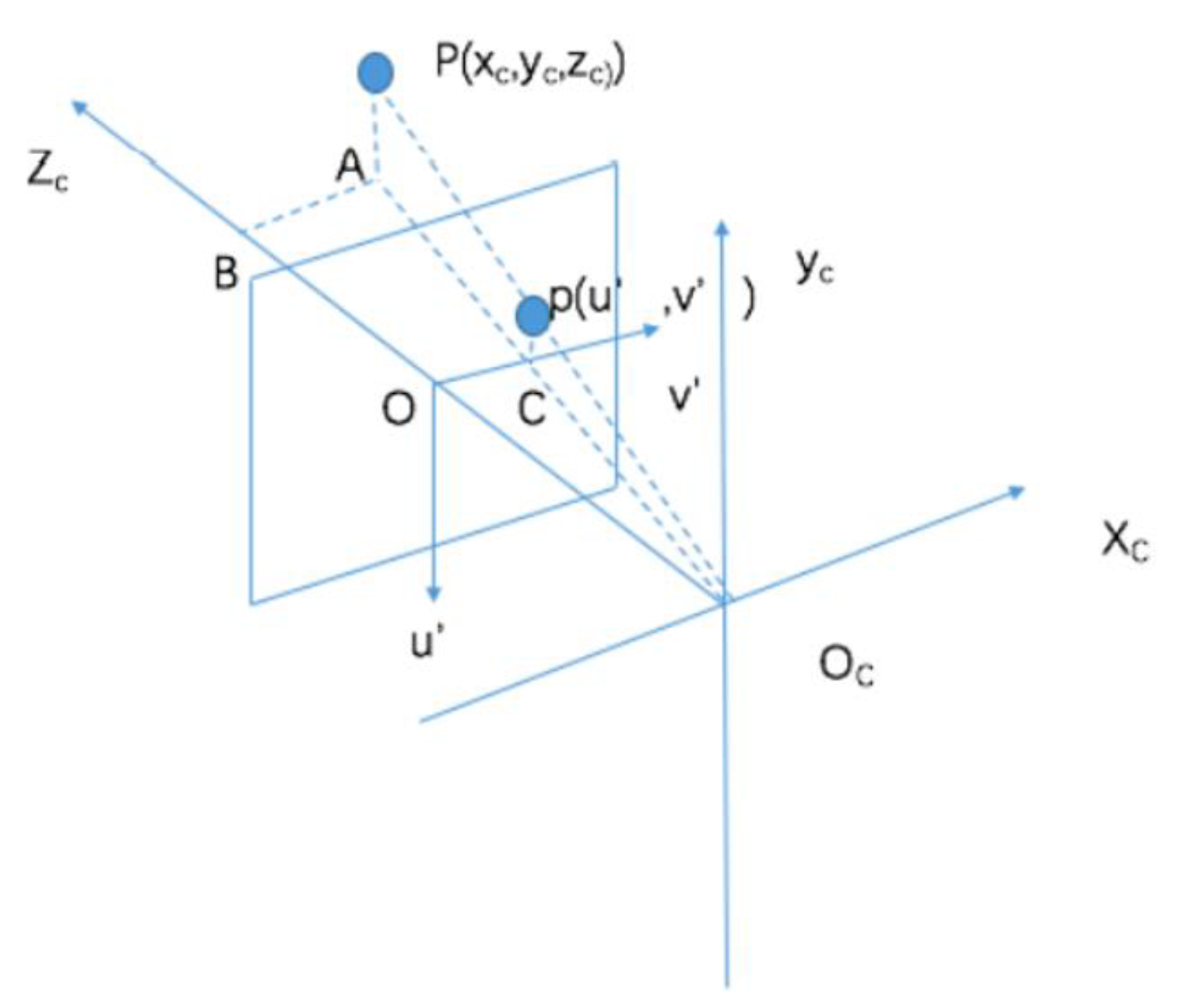
- The world coordinate system is an expression of the coordinate system of the objectively existing world. Its origin and scale unit can be arbitrary, and it is used to express the object information imaged by the camera. In a surveillance video system, the world coordinate system is constructed based on the monitoring field of view, and can be customized according to user needs. The camera model uses ().
- 2.
- The camera coordinate system is a camera-based coordinate system. Its origin is located at the optical center of the camera imaging lens, the x-axis and y-axis are parallel to the u’ and v’ axes of the image plane coordinate system, the z-axis is perpendicular to the x-axis, and the y-axis is parallel to the optical axis of the camera, forming a three-dimensional coordinate system inside the camera, represented by (). The world coordinate system is transformed to the camera coordinate system by a rigid body transformation.
- 3.
- The image-plane coordinate system is a two-dimensional coordinate system on the imaging plane. The origin is the line between the optical center and the optical axis, and its u’ and v’ axes are parallel to the u and v axes of the pixel coordinates, respectively. The distance from the origin of the image-plane coordinate system to the origin of the camera coordinate system is determined by the focal length of the camera.
- 4.
- The pixel coordinate system takes the upper-left corner of the image and the two mutually perpendicular sides of the image to form the u-axis and the v-axis as the origin.
3.2. Stereo Space Restoration Optimization Algorithm Based on Vanishing Point
3.2.1. Basic Algorithm
3.2.2. Optimization Method
| Algorithm 1. Optimization algorithm based on vanishing point calibration |
| Require: learning rate , Initial parameters ,, , , The maximum number of iteration rounds N, Small constant Repeat: Calculation error: A sample is randomly selected from the known control points, and the corresponding pixel coordinates are: Gradient calculation: , , , Parameter update: , , , Calculate new error: Iteration rounds: n = n + 1 Until: |
3.3. Stereo Grid Space Geometry Construction
3.3.1. Algorithm for Mapping Latitude and Longitude Coordinates to World Coordinate System
3.3.2. GeoSOT-3D Grid Code Construction Method
- Calculate longitude code
- Calculate latitude code
- Calculate height code
- Calculate longitude
- Calculate latitude
- Calculate height
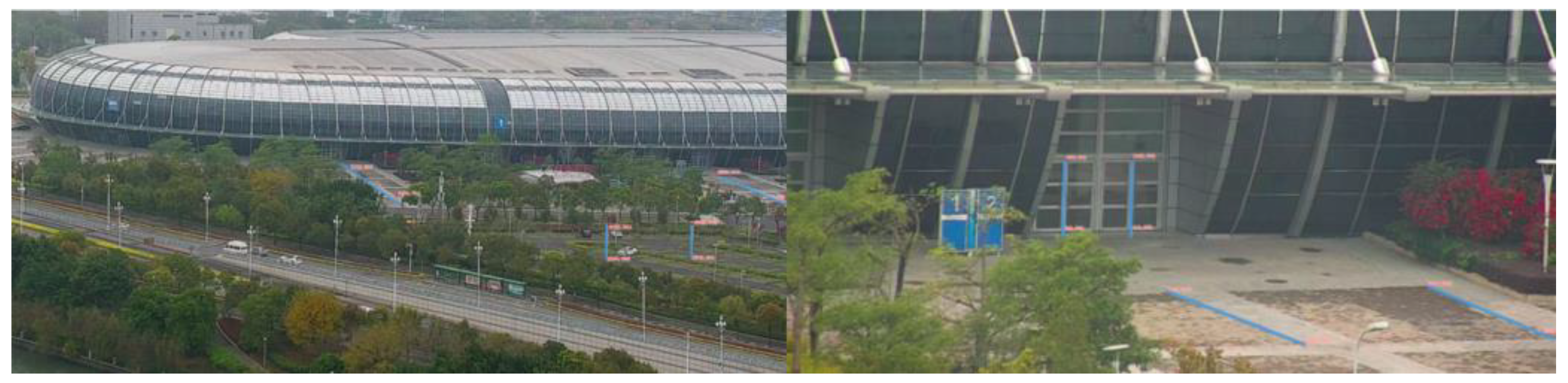
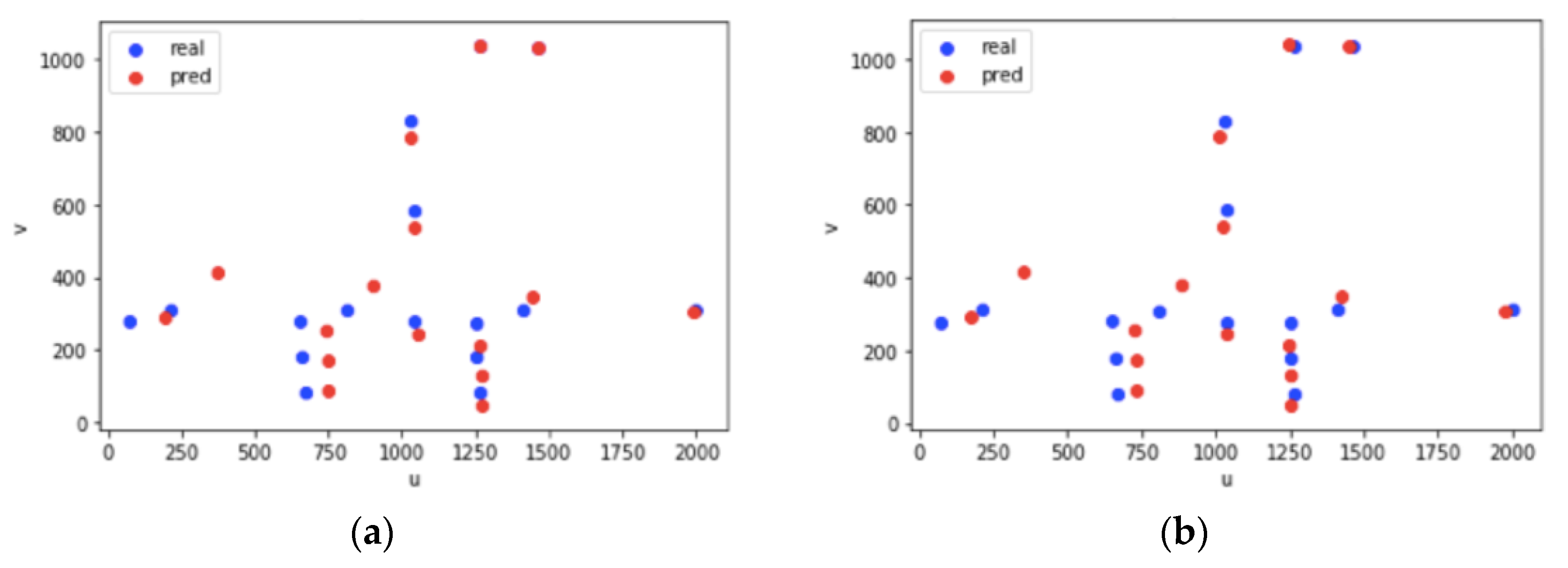
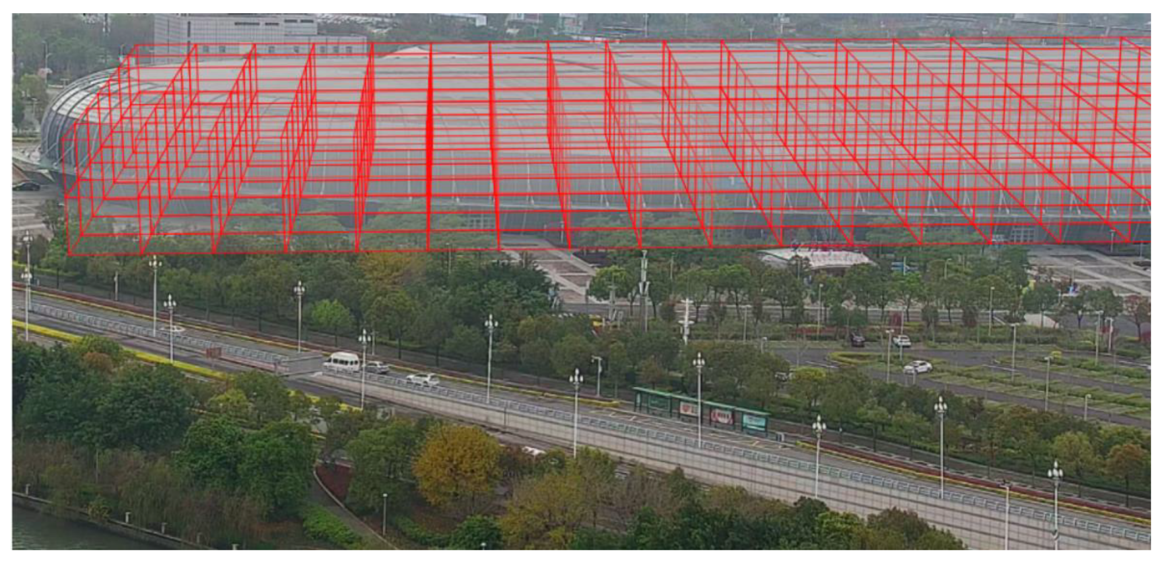
4. Results
5. Discussion
6. Conclusions
Author Contributions
Funding
Data Availability Statement
Conflicts of Interest
References
- Botín-Sanabria, D.M.; Mihaita, S.; Peimbert-García, R.E.; Ramírez-Moreno, M.A.; Ramírez-Mendoza, R.A.; Lozoya-Santos, J.D.J. Digital twin technology challenges and applications: A comprehensive review. Remote Sens. 2022, 14, 1335. [Google Scholar] [CrossRef]
- Sagar, M.; Miranda, J.; Dhawan, V.; Dharmaraj, S. The Growing Trend of Cityscale Digital Twins around the World. 2020. Available online: https://opengovasia.com/the-growingtrend-of-city-scale-digital-twins-around-the-world/ (accessed on 25 April 2022).
- Wu, Y.; Shang, J.; Xue, F. Regard: Symmetry-based coarse registration of smartphone’s colorful point clouds with cad drawings for low-cost digital twin buildings. Remote Sens. 2021, 13, 1882. [Google Scholar] [CrossRef]
- Lee, A.; Lee, K.; Kim, K.; Shin, S. A geospatial platform to manage large-scale individual mobility for an urban digital twin platform. Remote Sens. 2022, 14, 723. [Google Scholar] [CrossRef]
- Ketzler, B.; Naserentin, V.; Latino, F.; Zangelidis, C.; Thuvander, L.; Logg, A. Digital twins for cities: A state of the art review. Built Environ. 2020, 46, 547–573. [Google Scholar] [CrossRef]
- Cheng, C.Q. An Introduce to Spatial Information Subdivision Organization; Science Press: Beijing, China, 2012. [Google Scholar]
- Mimouna, A.; Alouani, I.; Khalifa, A.B.; El Hillali, Y.; Taleb-Ahmed, A.; Menhaj, A.; Ouahabi, A.; Amara, N.E.B. OLIMP: A heterogeneous multimodal dataset for advanced environment perception. Electronics 2020, 9, 560. [Google Scholar] [CrossRef]
- Ma, X.; Cheng, J.; Qi, Q.; Tao, F. Artificial intelligence enhanced interaction in digital twin shop-floor. Procedia CIRP 2021, 100, 858–863. [Google Scholar] [CrossRef]
- Haneche, H.; Boudraa, B.; Ouahabi, A. A new way to enhance speech signal based on compressed sensing. Measurement 2020, 151, 107–117. [Google Scholar] [CrossRef]
- Mahdaoui, A.E.; Ouahabi, A.; Moulay, M.S. Image denoising using a compressive sensing approach based on regularization constraints. Sensors 2022, 22, 2199. [Google Scholar] [CrossRef]
- Ferroukhi, M.; Ouahabi, A.; Attari, M.; Habchi, Y.; Taleb-Ahmed, A. Medical video coding based on 2nd-generation wavelets: Performance Evaluation. Electronics 2019, 8, 88. [Google Scholar] [CrossRef]
- He, F. Intelligent video surveillance technology in intelligent transportation. J. Adv. Transp. 2020, 2020, 8891449. [Google Scholar] [CrossRef]
- Brown, M.; Majumder, A.; Yang, R. Camera-based calibration techniques for seamless multiprojector displays. IEEE Trans. Vis. Comput. Graph. 2005, 11, 193–206. [Google Scholar] [CrossRef] [PubMed]
- Sun, J.; Wang, P.; Qin, Z.; Qiao, H. Overview of camera calibration for computer vision. In Proceedings of the 11th World Congress on Intelligent Control and Automation, Shenyang, China, 29 June–4 July 2014. [Google Scholar]
- Saeifar, M.H.; Nia, M.M. Camera calibration: An overview of concept, methods and equations. Int. J. Eng. Res. Appl. 2017, 7, 49–57. [Google Scholar] [CrossRef]
- Abdel-Aziz, Y.I.; Karara, H.M. Direct linear transformation from comparator coordinates into object space coordinates in close-range photogrammetry. Photogramm. Eng. Remote Sens. 2015, 81, 103–107. [Google Scholar] [CrossRef]
- Shih, S.W.; Hung, Y.P.; Lin, W.S. Efficient and accurate camera calibration technique for 3-D computer vision. In Optics, Illumination, and Image Sensing for Machine Vision VI; International Society for Optics and Photonics: Bellingham, WA, USA, 1992. [Google Scholar]
- Zhang, Z. A flexible new technique for camera calibration. IEEE Trans. Pattern Anal. Mach. Intell. 2000, 22, 1330–1334. [Google Scholar] [CrossRef]
- Hu, Z.Y.; Wu, F.C. Camera calibration method based on active vision. Chin. J. Comput. 2002, 11, 1149–1156. [Google Scholar]
- Triggs, B. Autocalibration and the absolute quadric. In Proceedings of the IEEE Computer Society Conference on Computer Vision and Pattern Recognition, San Juan, PR, USA, 17–19 June 1997. [Google Scholar]
- Caprile, B.; Torre, V. Using vanishing points for camera calibration. Int. J. Comput. Vis. 1990, 4, 127–139. [Google Scholar] [CrossRef]
- Lee, S.C.; Nevatia, R. Robust camera calibration tool for video surveillance camera in urban environment. In Proceedings of the CVPR 2011 WORKSHOPS, Colorado Springs, CO, USA, 20–25 June 2011. [Google Scholar]
- Meizhen, W.; Liu, X.; Yanan, Z.; Ziran, W. Camera coverage estimation based on multistage grid subdivision. ISPRS Int. J. Geo-Inf. 2017, 6, 110. [Google Scholar]
- Zhang, X.G.; Liu, X.J.; Wang, S.N. Mutual mapping between surveillance video and 2D geospatial data. Geomat. Inf. Sci. Wuhan Univ. 2015, 40, 139–145. [Google Scholar]
- Li, W.; Jing, H.T.; Yuan, S.W. Research on geographic information extraction from video data. Sci. Surv. Mapp. 2017, 11, 96–100. [Google Scholar]
- Milosavljevic, A.; Rancic, D.; Dimitrijevic, A.; Predic, B.; Mihajlovic, V. Integration of GIS and video surveillance. Int. J. Geogr. Inf. Sci. 2016, 30, 2089–2107. [Google Scholar] [CrossRef]
- Milosavljevic, A.; Rancic, D.; Dimitrijevic, A.; Predic, B.; Mihajlovic, V. A method for estimating surveillance video georeferences. ISPRS Int. J. Geo-Inf. 2017, 6, 211. [Google Scholar] [CrossRef]
- Xie, Y.; Meizhen, W.; Liu, X.; Wu, Y. Integration of GIS and moving objects in surveillance video. ISPRS Int. J. Geo-Inf. 2017, 6, 94. [Google Scholar] [CrossRef]
- Zhang, X.; Hao, X.Y.; Li, J.S.; Li, P.Y. Fusion and visualization method of dynamic targets in surveillance video with geospatial information. Acta Geod. Cartogr. Sin. 2019, 48, 1415–1423. [Google Scholar]
- Wu, Y.X. Research on Video Map and Its Generating Method. 2018. Available online: https://kns.cnki.net/KCMS/detail/detail.aspx?dbname=CMFD201901&filename=1018292439.n (accessed on 25 April 2022).
- Li, S.Z.; Song, S.H.; Cheng, C.Q. Mapping Satellite-1 remote sensing data organization based on GeoSOT. J. Remote Sens. 2012, 16, 102–107. [Google Scholar]
- Sun, Z.Q.; Cheng, C.Q. True 3D data expression based on GeoSOT-3D ellipsoid subdivision. Geomat. World 2016, 23, 40–46. [Google Scholar]
- Meng, L.; Cheng, C.Q.; Chen, D. Terrain quantization model based on global subdivision grid. Acta Geod. Cartogr. Sin. 2016, 45, 152–158. [Google Scholar]
- Yuan, J. Research on Administrative Division Coding Model Based on GeoSOT Grid. Master’s Thesis, School of Earth and Space Sciences, Peking University, Beijing, China, 2017. [Google Scholar]
- Hu, X.G.; Cheng, C.Q.; Tong, X.C. Research on 3D data representation based on GeoSOT-3D. J. Peking Univ. Nat. Sci. Ed. 2015, 51, 1022–1028. [Google Scholar]
- Liu, J.F. Research on Digital Camera Calibration and Related Technologies. Master’s Thesis, Chongqing University, Chongqing, China, 2010. [Google Scholar]
- Yoshikawa, N. Spatial position detection of three-dimensional object using complex amplitude derived from Fourier transform profilometry. In Proceedings of the Information Photonics, Optical Society of America, Charlotte, NC, USA, 6–8 June 2005. [Google Scholar]
- Orghidan, R.; Salvi, J.; Gordan, M.; Orza, B. Camera calibration using two or three vanishing points. In Proceedings of the 2012 Federated Conference on Computer Science and Information Systems (FedCSIS), Wroclaw, Poland, 9–12 September, 2012; IEEE: Piscataway, NJ, USA, 2012. [Google Scholar]
- Kong, Y.Y. Fundamentals of Geodesy; Wuhan University Press: Wuhan, China, 2010. [Google Scholar]


| u | v | Lon | Lat | Height |
|---|---|---|---|---|
| 485 | 275 | 119.356096 | 26.030987 | 20.0 |
| 1520 | 322 | 119.356876 | 26.030922 | 20.0 |
| 789 | 231 | 119.356313 | 26.031290 | 20.0 |
| 1338 | 226 | 119.356755 | 26.031389 | 20.0 |
| 949 | 305 | 119.356447 | 26.030902 | 20.0 |
| 1190 | 623 | 119.356690 | 26.030652 | 0.0 |
| 2413 | 638 | 119.357597 | 26.030742 | 0.0 |
| 2295 | 640 | 119.357492 | 26.030730 | 0.0 |
| 378 | 576 | 119.356022 | 26.030765 | 0.0 |
| 1952 | 290 | 119.357228 | 26.031058 | 20.0 |
| 2457 | 502 | 119.357607 | 26.030835 | 10.0 |
| 2332 | 293 | 119.357521 | 26.031098 | 20.0 |
| 277 | 245 | 119.355923 | 26.031143 | 20.0 |
| 2153 | 332 | 119.357378 | 26.030923 | 20.0 |
| 1570 | 475 | 119.35694 | 26.030758 | 10.0 |
| 92 | 496 | 119.355755 | 26.031068 | 0.0 |
| u | v | Lon | Lat | Height |
|---|---|---|---|---|
| 1464 | 1034 | 119.357021 | 26.030674 | 0.0 |
| 1263 | 1038 | 119.356999 | 26.030674 | 0.0 |
| 653 | 281 | 119.356948 | 26.030732 | 6.5 |
| 1250 | 275 | 119.357006 | 26.030739 | 6.5 |
| 1039 | 279 | 119.356982 | 26.030733 | 6.5 |
| 1030 | 831 | 119.356982 | 26.030733 | 0.0 |
| 1039 | 585 | 119.356982 | 26.030733 | 3.0 |
| 810 | 310 | 119.356961 | 26.030703 | 6.5 |
| 1409 | 311 | 119.357021 | 26.030708 | 6.5 |
| 210 | 312 | 119.356902 | 26.030697 | 6.5 |
| 2001 | 312 | 119.357082 | 26.030715 | 6.5 |
| 70 | 279 | 119.356887 | 26.030726 | 6.5 |
| 1267 | 81 | 119.357006 | 26.030739 | 8.5 |
| 670 | 81 | 119.356948 | 26.030732 | 8.5 |
| 1255 | 180 | 119.357006 | 26.030739 | 7.5 |
| 660 | 179 | 119.356948 | 26.030732 | 7.5 |
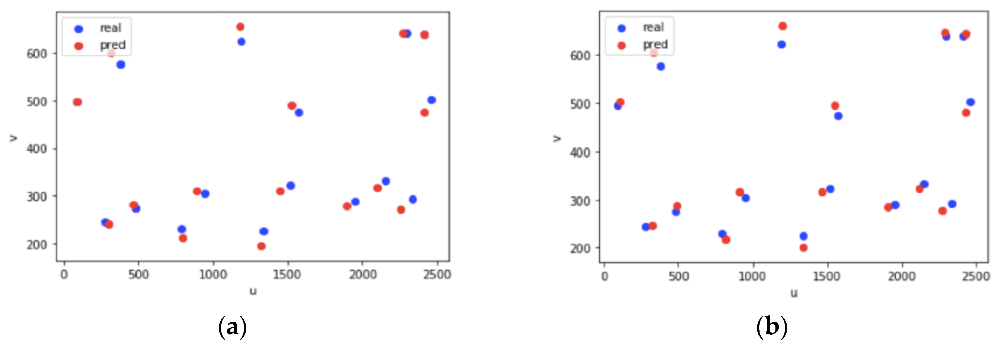
| Scenes | Control Point Error before Optimization | Control Point Error after Optimization | Error Rate after Optimization | Validation Point Error before Optimization | Verification Point Error after Optimization | Error Rate after Optimization |
|---|---|---|---|---|---|---|
| A | 5.917 | 5.858 | 1.06% | 6.974 | 6.183 | 1.13% |
| B | 1.119 | 1.110 | 2.52% | 1.089 | 0.945 | 2.10% |
| Grid Level | Control Point Error before Optimization | Control Point Error after Optimization | Validation Point Error before Optimization | Verification Point Error after Optimization |
|---|---|---|---|---|
| 21 | 9.515 | 9.515 | 0.0 | 0.0 |
| 22 | 7.974 | 8.416 | 6.546 | 6.546 |
| 23 | 5.146 | 5.567 | 7.187 | 7.187 |
| 24 | 5.648 | 5.648 | 6.870 | 5.879 |
| 25 | 5.943 | 5.943 | 7.041 | 6.226 |
| Control Point Error before Optimization | Control Point Error after Optimization | Validation Point Error before Optimization | Verification Point Error after Optimization | |
|---|---|---|---|---|
| 23 | 2.104 | 2.104 | 1.960 | 1.960 |
| 24 | 1.385 | 1.300 | 2.071 | 2.071 |
| 25 | 1.088 | 0.921 | 1.280 | 1.280 |
| 26 | 1.110 | 1.027 | 1.179 | 1.057 |
| 27 | 1.181 | 1.111 | 1.127 | 1.057 |
Publisher’s Note: MDPI stays neutral with regard to jurisdictional claims in published maps and institutional affiliations. |
© 2022 by the authors. Licensee MDPI, Basel, Switzerland. This article is an open access article distributed under the terms and conditions of the Creative Commons Attribution (CC BY) license (https://creativecommons.org/licenses/by/4.0/).
Share and Cite
Zhang, H.; Shi, R.; Li, G. RETRACTED: Geometric Construction of Video Stereo Grid Space. Remote Sens. 2022, 14, 2356. https://doi.org/10.3390/rs14102356
Zhang H, Shi R, Li G. RETRACTED: Geometric Construction of Video Stereo Grid Space. Remote Sensing. 2022; 14(10):2356. https://doi.org/10.3390/rs14102356
Chicago/Turabian StyleZhang, Huangchuang, Ruoping Shi, and Ge Li. 2022. "RETRACTED: Geometric Construction of Video Stereo Grid Space" Remote Sensing 14, no. 10: 2356. https://doi.org/10.3390/rs14102356
APA StyleZhang, H., Shi, R., & Li, G. (2022). RETRACTED: Geometric Construction of Video Stereo Grid Space. Remote Sensing, 14(10), 2356. https://doi.org/10.3390/rs14102356