Comparison between the Mesospheric Winds Observed by Two Collocated Meteor Radars at Low Latitudes

Abstract

This study compares the hourly mesospheric horizontal winds observed by two collocated and independent low-latitude meteor radars operating at 37.5 MHz and 53.1 MHz in Kunming, China (25.6°N, 103.8°E). Upon analyzing simultaneously detected meteor echoes, we find a fixed angular deviation between the baselines of the two meteor radar antenna arrays within the east–north–up coordinate system. Then, we correct the deviation in the antenna azimuth direction using a novel method and recalculate the horizontal zonal and meridional winds. A comparison of the results before and after the correction shows strong consistency between the winds observed by both meteor radars within the entire detection altitude range. Furthermore, we summarize the performance of different techniques for measuring mesospheric winds. Ultimately, our statistical analysis approach allows the uncertainties associated with meteor radar wind observations to be more precisely estimated.

1. Introduction

The mesosphere and lower thermosphere (MLT) region, which is widely accepted to be the region at altitudes between about 60 and 120 km, plays an important role in the coupling between the solar–terrestrial environment and the neutral atmosphere. The MLT region is dominated by dynamical coupling via atmospheric waves (including gravity waves, tides, and planetary waves) from below and by photoionization from above, caused mainly by the Sun [1,2]. These dynamics are reflected in the wind, temperature, and density of the atmosphere, so measuring these parameters of the neutral atmosphere can help characterize the transport of both momentum and energy within the MLT region [3].

Many techniques are applied to measure neutral winds in the MLT region, and most rely on remote sensing approaches. These include radio instruments (such as meteor radars (MRs), medium-frequency (MF) and high-frequency (HF) partial reflection radars (which utilize analysis using both the more common full-correlation analysis (FCA) and the imaging Doppler interferometer (IDI) analysis), and incoherent scattering radars) and optical instruments (such as LiDAR and Fabry–Pérot interferometers (FPIs)). Because of their compact size, easily understood operating principles, and automated operation [4,5], MRs are now the dominant method for acquiring continuous measurements of winds in the MLT region, and the long-term, continuous measurement of wind enables research on atmospheric dynamics [6,7,8] and climate change [9,10] in the MLT region. Nevertheless, given the diversity of the techniques available to investigate the MLT region, they should be accessible for calibration and validation to clarify their strengths and weaknesses, with the goal of better understanding real atmospheric phenomena. In this context, the intercomparison of MR observations with the results of other techniques can generally provide insights into the performance of MRs.

A joint measurement campaign involving two all-sky MRs was carried out from November 2013 to December 2014 at Kunming Station (25.6°N, 103.8°E). The results are of particular interest because there are very few collocated meteor radars capable of making measurements at the same time in the world. During the campaign, the two MRs operated simultaneously, providing a valuable opportunity to study the consistency among estimates of horizontal winds, the mesospheric density [11], and the atmospheric dynamics (tides, planetary waves) using the same detection principle.

In this study, we compare the neutral winds derived from the two collocated Kunming meteor radars (KMMRs) and discuss their consistency and internal errors. Then, we propose a novel but simple method to estimate and validate the angular deviation from the azimuth reference direction between the receiving arrays of the two KMMRs, and the method is verified using data recorded by the two radars. Our paper is organized as follows. In Section 2, we present the experiments and data sets. Then, in Section 3, we introduce the mathematical method for estimating the uncertainty. The results of a comparison and of a method for correcting the abovementioned angular deviation are discussed in Section 4, respectively, and we discuss other comparison cases in Section 5. Finally, we summarize our conclusions in Section 6.

2. Instruments and Data Sets

The Kunming meteor radar systems (KMMRs), which are operated by the China Research Institute of Radio Wave Propagation, belong to the Kunming Atmospheric Radar Facility [12] located at the Kunming Electromagnetic Environment Observation and Research Station (25.6°N, 103.8°E) in Yunnan Province, China. One of the two meteor radar systems at Kunming Station is a dedicated 37.5 MHz “all-sky” interferometric MR, essentially the same as that described by Holdsworth et al. [5], while the other is a 53.1 MHz stratospheric–tropospheric ST/MR similar to that described by Reid et al. [13]. The distance between the two MR antenna arrays is approximately 300 m, and the operating parameters for the two KMMRs are summarized in

Table 1. Main operating parameters of the two Kunming meteor radars.

Parameter	37.5 MHz	53.1 MHz
Pulse repetition frequency (PRF)	430 Hz	430 Hz
Peak power	20 kW	40 kW
Range resolution	1.8 km	1.8 km
Pulse type	Gaussian	Gaussian
Detection range	70–110 km	70–110 km
Pulse width	24 μs	24 μs

. Note that the two MRs are different only in regard to their operating frequency and peak power.

The data measured by the two KMMRs from 1 November 2013 to 31 December 2014, are used in this study. Both KMMRs are capable of providing hourly averaged zonal and meridional winds in the approximate altitude range of 70–110 km in height and temporal bins of 2 km and 1 h, respectively. Figure 1 illustrates an example of the meteor counts separately detected by the two KMMRs. The maximum meteor count was reached in the local morning (i.e., near 0100 UTC), while the fewest meteors were detected in the local afternoon (i.e., near 1000 UTC). In general, the 37.5 MHz MR detected more meteor echoes than the 53.1 MHz MR. The daily count rate is ~11,000 for the 37.5 MHz MR and ~9000 for the 53.1 MHz MR. The lower count for the higher frequency, even though it has a higher power, is consistent with the count being proportional to $P_T^{1/2}{\lambda }^{3/2}$, where $P_T$ is the transmitted power and $\lambda$ is the radar wavelength [14]. Figure 1b shows the height distributions of the meteor counts over a period of 426 days from 1 November 2013 to 31 December 2014; the meteor echoes detected at a zenith angle greater than 60 degrees are excluded. The height of the maximum meteor count for the 53.1 MHz MR is lower than that for the 37.5 MHz MR by approximately 3 km; this is because the meteor height distributions detected by lower-frequency MRs are characteristically higher than those detected by higher-frequency MRs [15,16].

3. Method

Using the approach proposed by Hocking [4], here we briefly describe the method employed to compare the same variables calculated using two different techniques. Denoting the two calculated winds as $\left\{x_i\right\}$ and $\left\{y_i\right\}$, i.e., the winds observed by two KMMRs, and the true wind value as $\left\{v_i\right\}$, we have:

$$x_i=v_i+\delta x_i,$$

(1)

$$y_i=g_0{v}_i+\delta y_i,$$

(2)

where $g_0$ is the assumed gain of the true wind in set $\left\{y_i\right\}$ relative to $\left\{v_i\right\},$ and $\delta x_i$ and $\delta y_i$ represent the random noise of the corresponding signal. We assume that $v_i$, $\delta x_i$, and $\delta y_i$ are independent of each other and that each follows a Gaussian distribution:

$$v_i ~ N\left(0, {\Sigma }_v^2\right),$$

(3)

$$\delta x_i ~ N\left(0,{\sigma }_x^2\right),$$

(4)

$$\delta y_i ~ N\left(0,{\sigma }_y^2\right).$$

(5)

Thus, the variance of the data sets $\left\{x_i\right\}$ and $\left\{y_i\right\}$ can be presented as:

$${\zeta }_x^2={\Sigma }_v^2+{\sigma }_x^2,$$

(6)

$${\zeta }_y^2=g_0^2{\Sigma }_v^2+{\sigma }_y^2.$$

(7)

Assuming that $\left\{x_i\right\}$ has no error, we can obtain the slope $g_x$ of the linear regression of $\left\{y_i\right\}$ fitted to $\left\{x_i\right\}$, and similarly we can obtain the slope $g_y$ of the linear regression of $\left\{x_i\right\}$ fitted to $\left\{y_i\right\}$. The reciprocal of $g_y$ is used here instead of $g_y$ to facilitate the following analysis. In addition, we can show that:

$${\sigma }_x={\zeta }_x{\left(1-\frac{g_x}{g_0}\right)}^{\frac{1}{2}},$$

(8)

$${\sigma }_y={\zeta }_y{\left(1-\frac{g_0}{g_y}\right)}^{\frac{1}{2}},$$

(9)

since ${\zeta }_x^2$ and ${\zeta }_y^2$ are simply the variances of the two data sets and $g_x$ and $g_y$ can be estimated easily by least squares regression. Consequently, the mathematical relationship among the three unknowns $g_0$, ${\sigma }_x$, and ${\sigma }_y$ can be expressed by Equations (8) and (9). In the following section, we employ this procedure to compare the MR-observed winds.

4. Results

4.1. Comparison between the Kunming 37.5 MHz and 53.1 MHz Meteor Radar Winds

Figure 2 presents the hourly mean horizontal winds observed by the 37.5 MHz and 53.1 MHz MRs from 8 November 2013 to 10 November 2013. The winds were calculated using the all-sky method. As shown in Figure 2a–d, the hourly winds observed by the two MRs are very similar, and both reflect a distinct diurnal tidal structure. The wind differences between the two MRs in Figure 2e–f still present a weak tidal structure, especially in the zonal component. We investigate the reasons for this below.

To compare the MR winds more intuitively, we quantitatively compared the parameters using Hocking’s method, as mentioned previously. Figure 3a shows a scatter plot of the meridional winds at a height of 86 km derived by the two KMMRs over a period of 14 months. The red line indicates the regression of the 53.1 MHz MR results on the 37.5 MHz MR results with slope $g_x$; likewise, the blue line shows the regression of the 37.5 MHz MR results on the 53.1 MHz MR results with slope $g_y$. As mentioned above, neither of these two slopes can represent the best fit of the data, since we performed least squares regression under the assumption that one of the two data sets contains no error. Nevertheless, these regressions could provide an estimate of the optimal slope $g_0$, as $g_x$ is smaller than $g_0$ and $g_y$ is greater than $g_0$. If we assume that both of the data sets contain the same random errors, i.e., ${\sigma }_x={\sigma }_y$, it is possible to calculate the optimal slope $g_0$ using the relationship among $g_0$, ${\sigma }_x$, and ${\sigma }_y$, which is plotted as the curve in Figure 3b. The value of $g_0$ lies between 0.96 and 1.08, indicating a high degree of similarity between the true wind velocities detected by these two MRs at 86 km. This curve allows us to identify the variance of both the 37.5 MHz MR and the 53.1 MHz MR. For example, the green dashed line in Figure 3b signifies ${\sigma }_x={\sigma }_y$, corresponding to the total least squares fitting estimate $g_0$ shown as the green line in Figure 3a, and the black dashed line gives an estimate of the variances of the two data sets (${\sigma }_x$, ${\sigma }_y$) assuming that $g_0=1$.

Figure 4a shows that the best-fitting slope $g_0$ for both the zonal and meridional components varies around approximately 1.0, which in a sense verifies our assumption that ${\sigma }_x={\sigma }_y$; this finding suggests that even if the random errors of the two systems may not be the same, they are close. Therefore, under the assumption that ${\sigma }_x={\sigma }_y$, $g_0$ does reflect the similarity between the real wind velocity variations in both sets of data. However, the variations in the two wind components are not the same; below 84 km, the slope $g_0$ is basically less than 1.0 for the meridional component and greater than 1.0 for the zonal component, while above 84 km the results are reversed, which indicates higher zonal true wind speeds of the 53.1 MHz MR below 84 km and higher meridional true wind speeds of the 37.5 MHz MR above 84 km.

In Figure 4b, $g_x$ and $g_y$ represent the linearly regressed slopes of the 53.1 MHz MR on the 37.5 MHz MR and those of the 37.5 MHz MR on the 53.1 MHz MR, respectively. The values of these slopes are similar to the values of $g_0$ shown in Figure 4a. The meridional results nearly reach 1.0 at altitudes with large meteor counts, suggesting that the meteor echo rate could affect the reliability of the calculated horizontal winds. In contrast, the zonal results change little with height.

Figure 4c shows the estimated values of ${\sigma }_x$ and ${\sigma }_y$ under the assumption that ${\sigma }_x={\sigma }_y$. The random errors of the zonal and meridional components both decrease below 86 km and increase above 86 km. This can reasonably be explained by the fact that the meteor counts detected by the two MRs basically follow a Gaussian distribution and peak at a height of approximately 86 km.

The RMS errors of the wind velocity are presented in Figure 4d. Here, the continuous RMS error is used. The RMS errors of the two systems exhibit the same tendency over the considered height range, indicating that the distributions of the wind velocities measured by the two MRs are basically the same. Furthermore, the RMS error on the meridional component is larger than that on the zonal component. We should note that the RMS error consists of random noise and the geophysical variations in wind, and considering these sources of error gives us the ability to deduce the tendency of the true wind variance. For instance, on the meridional component, the random noise decreases over the height range of 78–86 km, while the RMS error continues to increase, indicating that the meridional wind variance must increase with height within this height range to maintain the equality of the variance. In contrast, on the zonal component, the tendencies of the random noise and RMS error are almost consistent; thus, the standard deviation of the actual zonal wind remains nearly constant with height.

Figure 4e shows the random errors of ${\sigma }_x$ and ${\sigma }_y$ when $g_0=1$. The results on both the zonal and meridional components indicate small and nearly equal inherent random errors for both MRs. Recall that the expressions of the variance for the two data sets are composed of the signal variance and random error; hence, we can now estimate the random error of each MR system. It seems that the zonal (${\sigma }_x$) and meridional (${\sigma }_y$) errors appear to increase with altitude and seem to be independent of the meteor count, which contradicts the trends shown in Figure 4c.

It is obvious that the correlation coefficients of the two MRs are close to 1.0, with most of them exceeding 0.8. Notably, there is a higher correlation for the meridional component than for the zonal component, and the correlation for the latter does not change much with height, while that for the former varies by ~0.15 over the entire height range. This is interesting because the correlation coefficient generally rises when the meteor counts increase; thus, whereas the meridional results are reasonable, the zonal results should be viewed with scepticism.

4.2. Comparison with Corrected Winds

4.2.1. Proposed Method for Correcting the Antenna Angular Deviation

It is worth noting that ${\sigma }_x$ and ${\sigma }_y$ are intended to signify the measurement errors in each technique. However, it is not possible for two systems, even when they are collocated, to obtain identical measurements. To facilitate a more precise comparison, we established criteria to select the meteor echoes detected simultaneously by both KMMRs so that we can reduce the effects of meteor echoes detected at different times and locations. Considering the MR resolution, we chose meteors using spatial bins with dimensions of 3° (azimuth) by 3° (zenith) by 3 km (altitude) and a temporal bin of 3 s; any bins containing more than one meteor echo were discarded [16,17]. However, we retained only 2012 meteor echoes after applying these criteria, which was far fewer than anticipated.

To investigate further, we changed the thresholds of the zenith and azimuth angles and confirmed that the azimuth angle did influence the count of chosen meteor echoes, indicating that the antenna array baselines of the two MRs may not be parallel. To find the angular deviation between these two antenna arrays, we implemented the following processing steps to correct the azimuth data: (1) first, we selected the meteor echoes that matched the criteria mentioned above, excluding the azimuth criterion; (2) second, we calculated the difference between the azimuth angles of the two data sets corresponding to the selected meteor echoes and computed the histogram of the angular deviation; (3) third, Gaussian fitting was performed on the histogram to obtain the mean and standard deviation of the deviation, where the former basically represents the relative angular deviation between the azimuth reference direction of the two MR receiving arrays; (4) finally, the mean angular deviation was added to or subtracted from one or both data sets, and then steps 2 and 3 were repeated to ensure that the statistical mean was approximately 0. In this way, the systematic error associated with the deviation from the azimuth reference direction was calibrated, facilitating the subsequent retrieval of winds. Nevertheless, we should note that this method is capable only of identifying and correcting the relative angular bias, whereas the absolute bias needs to be validated by an additional technique.

Figure 5 shows the statistical differences in the azimuth and zenith using the method described above. We find that the meteor echoes observed simultaneously by the two MRs reaches a maximum when the angular differences are set to approximately 17° and 0° in the azimuth and zenith directions, respectively, which indicates that the baselines of the two antenna arrays have different azimuthal baselines. To confirm our estimate of this deviation, we employed the Global Positioning System (GPS) to measure the true direction of the 53.1 MHz MR antenna array, revealing that the 53.1 MHz antenna array deviates by 2.4° from true east and north. As for the 37.5 MHz MR, it was operated only until December 2014, after which it was moved to Manzhouli City (49.56°N, 117.52°E), China; thus, we cannot directly measure the true orientation of this antenna array. Nevertheless, based on our estimation of 17° between the two KMMRs, we presume that the 37.5 MHz MR antenna array deviated by 14.6° from true east and north. The deviations of the receiver’s local coordinates from the actual ENU coordinate system will affect the obtained azimuth data, and then affect the wind estimation. Figure 6 plots schematics illustrating the angular deviations for these two MR antenna arrays. The green curve in Figure 5a represents the azimuth deviation of simultaneously observed meteor echoes after rotating the observation system 14.6° counterclockwise for the 37.5 MHz MR and 2.4° clockwise for the 53.1 MHz MR by correcting the corresponding azimuth data. The number of simultaneous meteor echoes reaches the maximum near 0°, as expected, which means that the directions of the two antenna arrays should be in the same coordinate system. Therefore, we now seek to identify possible ways to improve MR observations through the proposed angular correction method.

4.2.2. Comparison of the Wind Results after an Angular Correction

Measurements of the angle of arrival can directly affect the estimation of horizontal winds [18,19]. Knowing the angular deviations of the two MR antenna arrays, we recalculated the horizontal winds. Figure 7 shows a comparison of the hourly horizontal winds after correcting the azimuth reference direction. Compared to the results in Figure 2, the corrected winds show stronger consistency between the two MRs; specifically, the wind differences are smaller. Moreover, the tidal structures in the zonal and meridional wind differences observed in Figure 2e,f are both effectively eliminated. This indicates that the tidal variation can be accurately captured by the two MRs. The reduced wind differences also mean that both MR systems can accurately observe consistent geophysical variations after correcting this systematic error.

Figure 8 quantitatively summarizes the comparisons of the corrected winds. Compared to Figure 4a, the results are closer to what we expected, especially the zonal results. The values of $g_0$ in Figure 8a are much closer to 1, and the variation range of $g_0$ changes from [0.86, 1.02] to [0.94, 1.02] after the correction. Similarly, in Figure 8b, $g_x$ and $g_y$ are closer to 1, even at low and high altitudes. In Figure 8c, the equal value ${\sigma }_x={\sigma }_y$ is significantly decreased by approximately 20%. The RMS errors do not significantly change because the angular correction basically makes the wind direction more accurate, and the changes for the zonal and meridional RMS of the 53.1 MHz MR are less than ~0.1. Comparing these two wind components reveals that the meridional wind variance is higher than the zonal wind variance. The values of ${\sigma }_x$ and ${\sigma }_y$ when $g_0=1$ all decrease as the meteor count increases, indicating that the zonal ${\sigma }_x$ and meridional ${\sigma }_y$ results in Figure 4e are artifacts caused by systematic errors.

Figure 9 shows the distribution of the differences between the calculated winds from the two MRs at each height before and after the angular correction. The wind difference after the angular correction is much smaller than before. First, we find that the mean values of both the zonal and meridional wind differences after the angular correction are close to 0 within the entire detection altitude range. Second, the standard deviation of the wind difference is much smaller than that before the angular correction. These results indicate that by correcting the deviation in the azimuth reference direction and recalculating the winds, we can successfully calibrate the measurement errors between the two systems and more accurately estimate the systematic errors of the MRs. It is, therefore, reasonable to conclude that the wind uncertainties estimated for two collocated and independent MRs can help to better understand the MR technique.

Additionally, the winds are measured by the two MRs over a year, so here we briefly discuss the seasonal variations of the mean differences and standard deviations. The monthly mean wind differences and the corresponding standard deviations are shown in Figure 10, and the monthly meteor counts are included due to the significant effects on the wind estimation. The meteor counts show the characteristics of seasonal variations, while the mean differences and standard deviations have no distinct seasonal variation. Additionally, the variations of the mean differences and the corresponding standard deviations seem to be affected by the meteor counts. In December 2013 and May 2014, the meteor counts of both MRs are sufficient and close, and the corresponding mean differences seem to be close to 0. However, we cannot draw such a conclusion that the meteor counts dominant the variations of the mean differences and the corresponding standard deviations, since the meteor counts in June and July are nearly the same but the corresponding mean differences are different, which will require further research.

5. Discussion

The results shown in Figure 9 after applying the angular correction present better agreement and smaller variances than those before the correction.

Table 2. Statistics of several comparison cases.

Case	Height Range (km)	Wind Component	Correlation	$\mathbf{Slope}{\mathit{g}}_0$	Mean Difference (m/s)	Standard Deviation (m/s)	Instruments (x and y) and Sites (Lat, Lon)
This study	76–94	Zonal	0.92–0.96	0.98–1.02	−0.43–0.55	6.03–11.23	37.5 MHz and 53.1 MHz MRs, Kunming (25.6°N, 103.8°E)
		Meridional	0.87–0.97	0.94–1.00	−0.03–0.60	5.89–11.24
Reid et al. (2018) and McIntosh (2010)	80–98	Zonal	0.60–0.78	1.05–1.24	−1.82–1.94	13.64–17.16	33.2 MHz and 55 MHz MRs, Davis (69°S, 78°E)
		Meridional	0.45–0.85	0.98–1.23	1.08–3.85	12.83–23.91
Reid et al. (2018) and McIntosh (2010)	80–98	Zonal	0.5–0.8	0.38–0.95	−1–4.5	14.7–27.5	33.2 MHz MR and 1.98 MHz MF radar (O-mode), Davis (69°S, 78°E),
		Meridional	0.5–0.8	0.37–0.85	0.8–4.2	13.2–28.5
		Zonal	0.5–0.8	0.48–1.12	−1–6.8	16–25	55 MHz MR and 1.98 MHz MF radar (FCA), Buckland Park (34.6°S, 138.5°E)
		Meridional	0.5–0.8	0.8–1.22	−4–1.5	15–23
Cervera and Reid (1995)	80–98	Zonal	N/A	0.38 (>90 km), 0.80 (<90 km)	−12.6–5.9	11.7–26.5	Narrow beam MR and 1.98 MHz MF radar, Buckland Park (34.6°S, 138.5°E)
Jones et al. (2003)	80–95	Zonal	N/A	N/A	2.0–7.8	16.7–26.4	MR and IDI, Bear Lake Observatory (41.9°N, 111.4°W)
		Meridional
Liu et al. (2002)	86, 93	Zonal	0.84, 0.95	0.816, 1.149	−1.6, 5.6	>20, >30	Lidar and MR, Kirtland Air Force Base (35°N, 106.5°W)
		Meridional	0.93, 0.88	0.675, 0.801	−3.1, 4.8	>20, >20
Franke et al. (2005)	82–98	Zonal	0.89	N/A	−0.2	N/A	Lidar and MR, Maui (20.75°N, 156.43°W)
		Meridional	0.91	N/A	0.8	N/A
Lee et al. (2021)	87, 97	Zonal	0.92, 0.83	0.78, 0.79	−0.7, −1.1	>20, >30	MR and FPI, King Sejong Station (KSS) in Antarctica (62.22°S, 58.79°W)
		Meridional	0.88, 0.86	0.88, 0.62	−1.2, −2.9	>20, >30
Gu et al. (2021)	85–89	Zonal	0.76–0.88	1.31	N/A	N/A	FPI and MR, Kunming (25.6°N, 103.8°E)
		Meridional	0.75–0.91	1.31

N/A: Not Available.

summarizes the conclusions of previous studies that performed mesospheric wind comparisons between MRs and other ground-based techniques (e.g., other MRs, lidars, MF radars, IDIs, and FPIs). Our results are similar to those obtained by Reid et al. [20] and McIntosh [21], who conducted comparisons of the hourly averaged neutral winds derived from two MRs operating at 33.2 and 55 MHz at Davis Station (68.6°S, 77.9°E), Antarctica. However, the two KMMRs achieved better performance in estimating the wind uncertainties. In general, compare to the Davis MRs results, this study shows higher correlation coefficients (by ~0.15) at much closer to a gain ratio $g_0$ of 1 (by ~0.1), smaller mean wind differences (less than 1 m/s), and reduced standard deviation (by half). This may be because the 53.1 MHz KMMR has a much higher meteor count rate (approximately 9000 per day) than the 55 MHz MR at Davis Station (only approximately 500–2000 per day because operation is interleaved with other experiments) [22]. On the other hand, factors such as the seasonal variations, geophysical phenomena (e.g., tides and gravity waves) and system configuration between the low (Kunming Station) and high (Davis Station)-latitude sites are also contributors to meteor wind estimates. However, this is beyond the scope of this paper, and we leave this for future work.

Reid et al. [20], Vincent et al. [23], and McIntosh [21] also conducted comparisons of the wind measurements observed by the MRs and the collocated MF radars at Davis Station (high-latitude) and Buckland Park (mid-latitude), respectively, in the Southern Hemisphere. Their results indicated that the MF radar winds at both sites were clearly underestimated compared with the MR measurements. The similar wind comparisons between MRs and MF radars presented by Cervera and Reid [24] and Hall et al. [25] all indicated good correlations between MF radar and MR winds and suggested that MF radars might underestimate the retrieved winds by up to 20% at some heights. Jones et al. [26] compared the winds observed over a four-month period by an IDI and MR at Bear Lake Observatory (41.9°N, 111.4°W) and found good agreement between the two measurements consistent with MF and meteor radar intercomparisons. However, it is important to note that the quality of IDI measurements depend strongly on the experimental configuration, as discussed by Holdsworth and Reid [27] and Reid [2]. The reasons for the underestimation are discussed at length by Reid [2], who notes that the underestimation varies depending on the radar and the analysis applied and varies with height over their observing range (typically 60–94 km by day; 78–94 km by night). There are several very long-term and valuable MF radar data sets for which correction factors can be calculated, at least in the 75 to 94 km height region where they overlap with the MR coverage. Therefore, intercomparisons with MR measurements can provide a reference for the validation and calibration of these MF radar data.

There are many other intercomparisons with MRs in the literature. For example, Liu et al. [28] and Franke et al. [29] compared the wind measurements from lidar and MR systems and found a strong correlation with reasonable RMS differences between these two techniques. They also suggested that both instruments can precisely capture large-scale variabilities such as tides and planetary waves; however, the two techniques measure the atmosphere with different viewing geometries, causing them to exhibit different sensitivities to gravity waves.

Lee et al. [30] compared the winds at the two altitudes of 87 and 97 km retrieved by using the OH and OI emissions observed by the FPI and MR at King Sejong Station in Antarctica (62.22°S, 58.79°W), and they suggested that the two wind measurements agree well. In addition, Gu et al. [31] conducted a comparison between the winds at 87 km observed by the Kunming FPI (OH emission) and the 53.1 MHz MR and similarly indicated a good correlation between the two techniques; moreover, they also reported that the FPI estimates were smaller than the MR measurements by about 30%, and the bias was larger than for MF radar winds.

The statistical results summarized herein affirm the comparability of other devices with MRs in the retrieval of winds in the MLT region. Moreover, this work verifies the reliable consistency in the performance of MRs at different operating frequencies and demonstrates the utility of MRs in observing the MLT region.

6. Summary

In this work, we perform a series of comparisons of the wind measurements at two collocated MRs in Kunming, China (25.6°N, 103.8°E), and we propose a method to correct the angular deviation between the baselines of the two systems. The parameters used to compare the wind measurements are obtained mainly by least squares regression. The main points are summarized as follows:

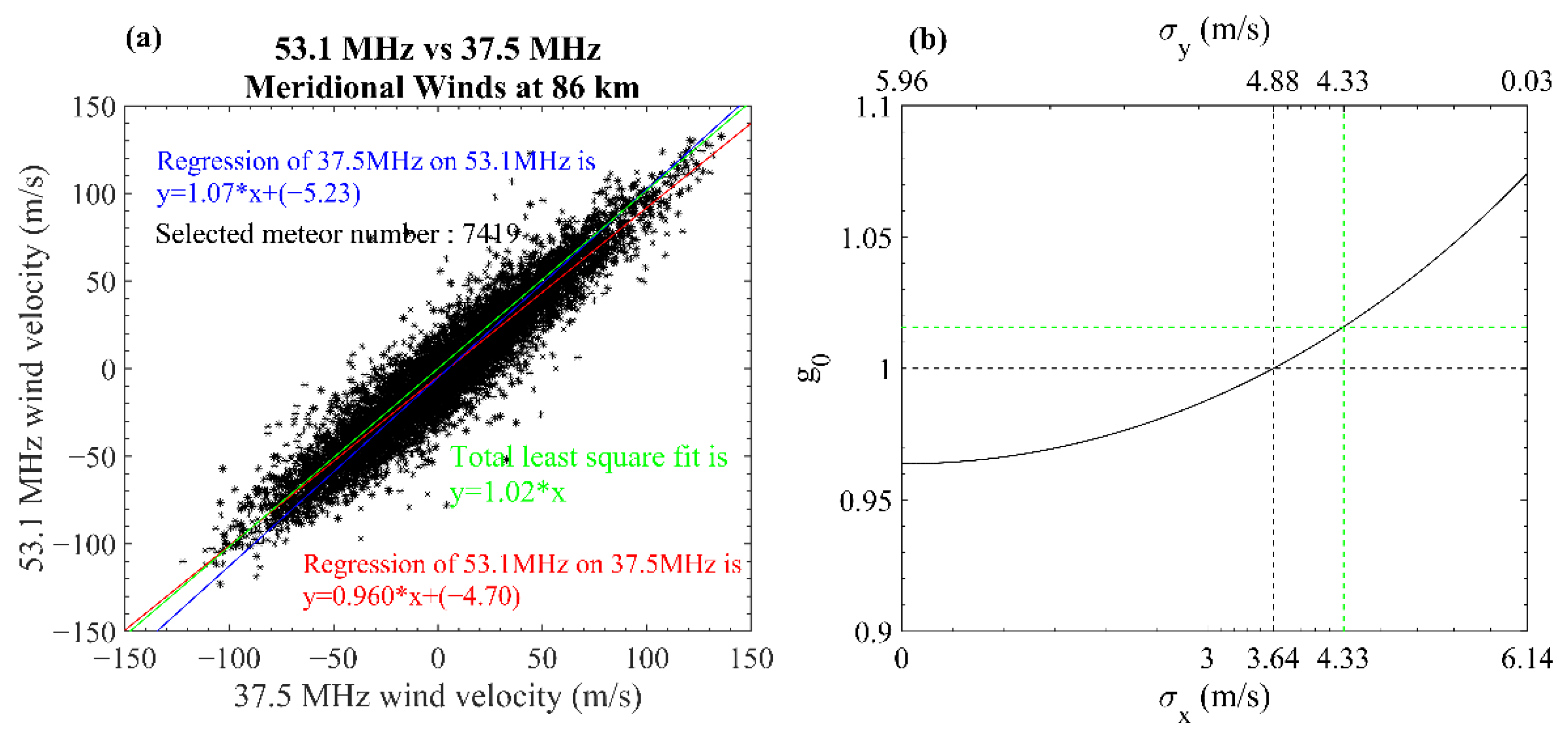
• Statistical analyses of the winds measured by the two MRs reveal an estimate of the uncertainties in the winds from the two systems, meaning the wind fields obtained by the different radars can be calibrated. The least squares regression fitting line is close to the y = x line, which means that the random errors of the two techniques are similar.
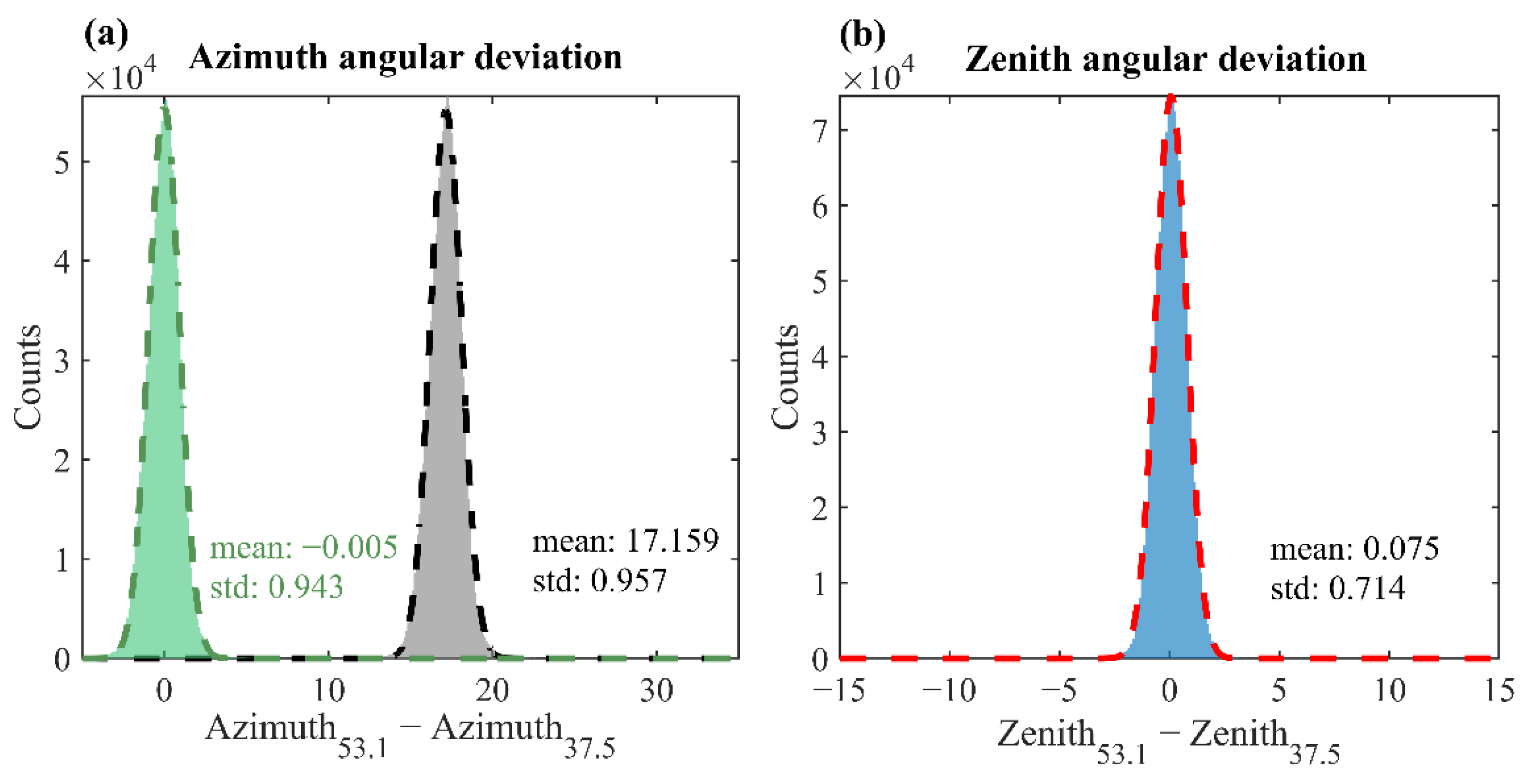
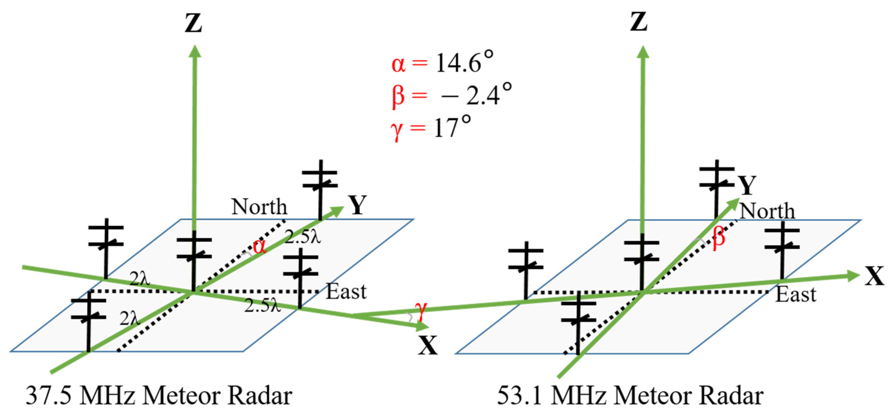
• Our correction method identifies the relative deviation between the reference directions of two collocated MR systems by selecting simultaneously observed meteors. This enables us to estimate the deviation in the azimuth reference direction. Fortunately, this method requires no additional hardware or data. After the correction has been implemented, the mean deviation between the reference directions of the two MR receiving systems approaches 0°; thus, the two systems can be regarded as being aligned. For these two MRs, correcting the angular deviation facilitates a qualitative and quantitative comparison, as well as the joint observation and verification of atmospheric dynamics in the MLT region, such as atmospheric tides and gravity waves.
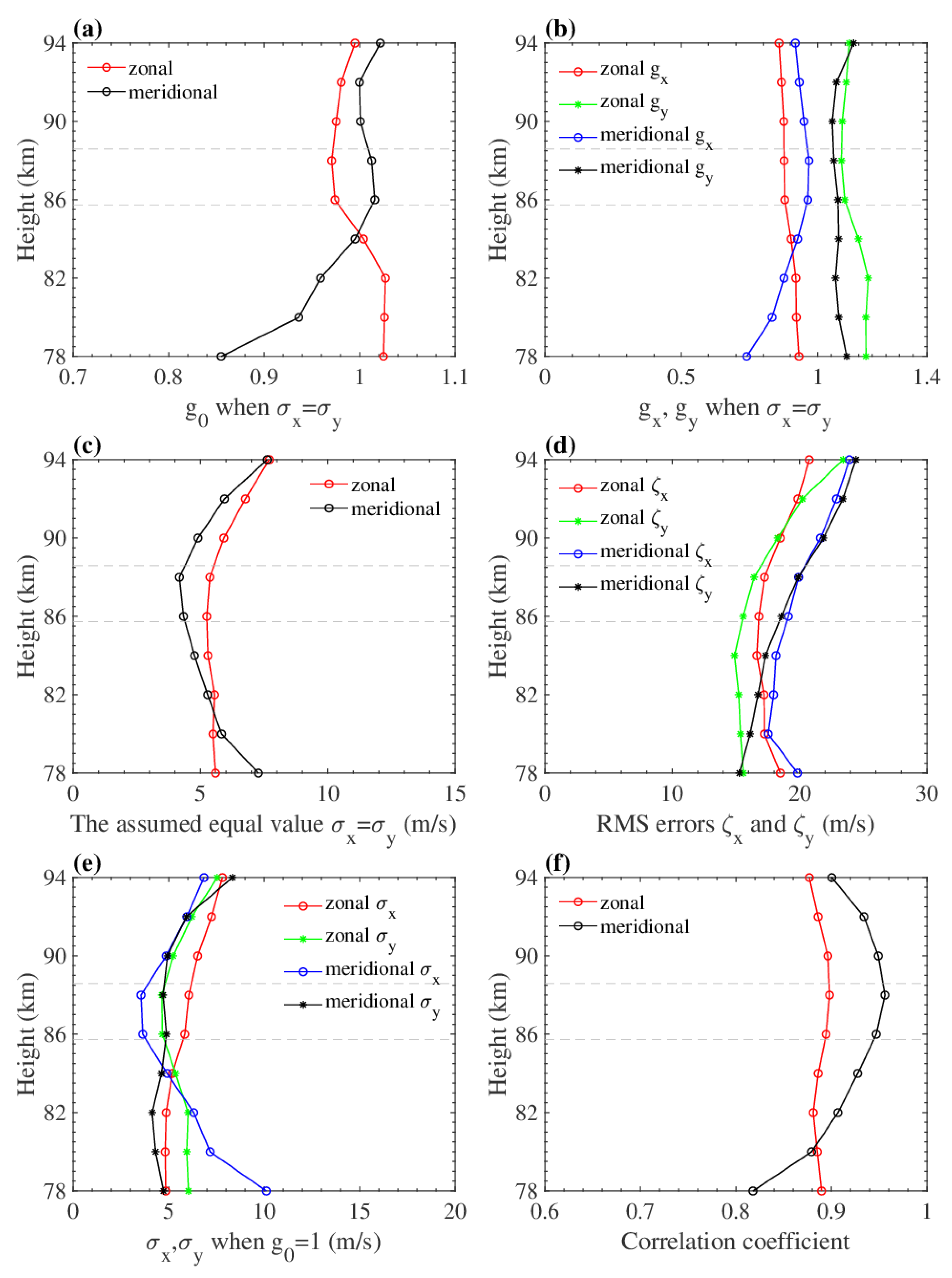
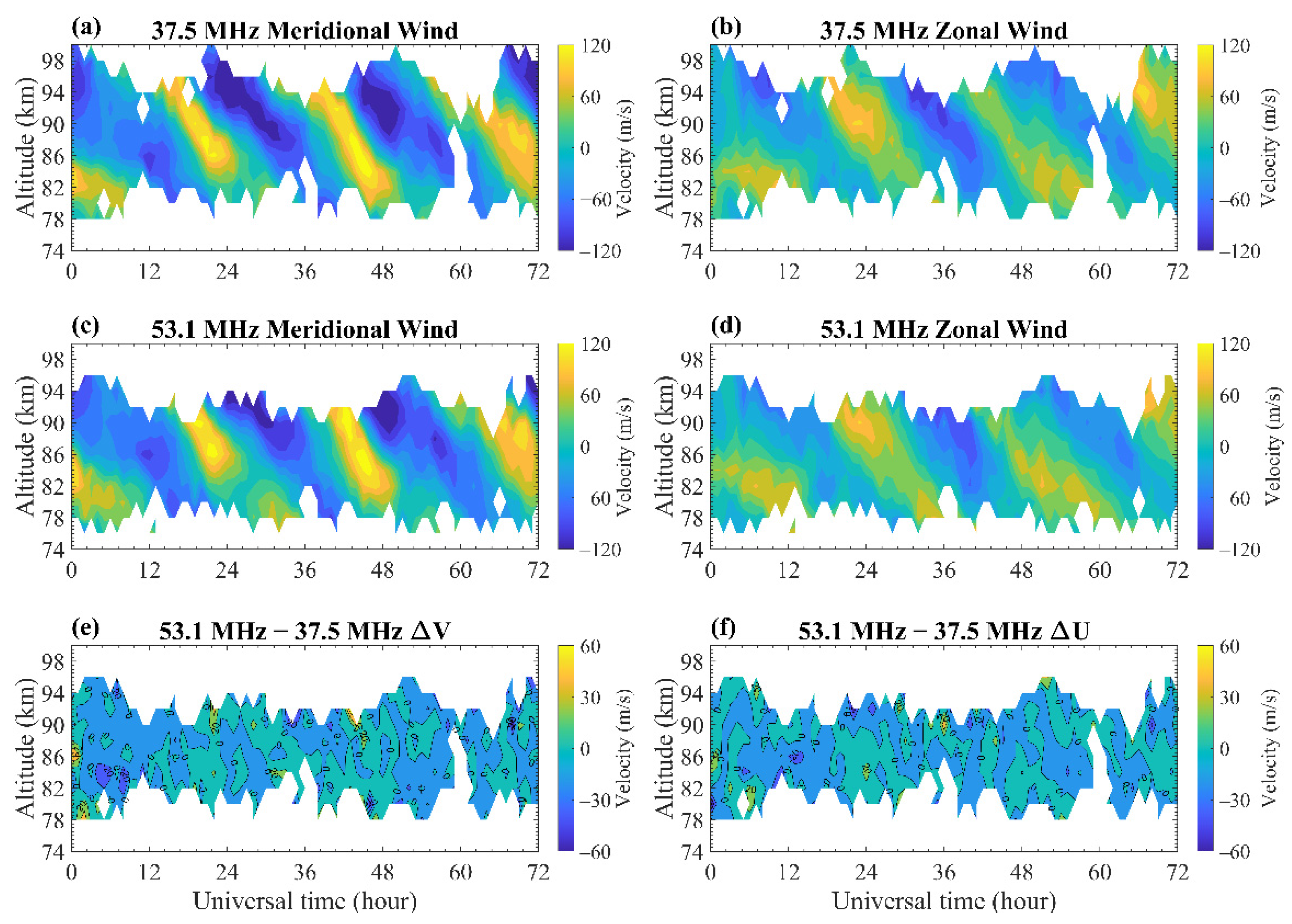
• The winds measured by the two collocated MRs show strong agreement. The results are highly correlated with the meteor distributions and are best at the peak height. Within the altitude range of 78–94 km, the correlation coefficients are higher than 0.78, and the wind velocities observed by the 53.1 MHz MR are generally lower than those observed by the 37.5 MHz MR by approximately 5–20%. After the angular deviation is corrected, the correlation coefficients increase by ~0.05 and are essentially greater than 0.9 over the entire height range. Furthermore, the uncertainties ${\sigma }_x$ and ${\sigma }_y$ are reduced by approximately 20%, and the differences in the wind components can basically be ignored. The comparison of the results from before and after implementing the correction confirms the consistent performance of both KMMRs for the entire detection height range. When compared to other techniques, MRs seem to provide a benchmark for MLT wind measurements, at least in this study within the altitude range of 78–94 km, where enough meteor counts are obtained.

References

1. Vincent, R.A. The dynamics of the mesosphere and lower thermosphere: A brief review. Prog. Earth Planet. Sci. 2015, 2, 4. [Google Scholar] [CrossRef] [Green Version]
2. Reid, I.M. MF and HF radar techniques for investigating the dynamics and structure of the 50 to 110 km height region: A review. Prog. Earth Planet. Sci. 2015, 2, 33. [Google Scholar] [CrossRef] [Green Version]
3. Sato, K.; Watanabe, S.; Kawatani, Y.; Tomikawa, Y.; Miyazaki, K.; Takahashi, M. On the origins of mesospheric gravity waves. Geophys. Res. Lett. 2009, 36, L19801. [Google Scholar] [CrossRef] [Green Version]
4. Hocking, W.K.; Thayaparan, T.; Franke, S.J. Method for statistical comparison of geophysical data by multiple instruments which have differing accuracies. Adv. Space Res. 2001, 27, 1089–1098. [Google Scholar] [CrossRef]
5. Holdsworth, D.A.; Reid, I.M.; Cervera, M.A. Buckland Park all-sky interferometric meteor radar. Radio Sci. 2004, 39, RS5009. [Google Scholar] [CrossRef]
6. Yu, Y.; Wan, W.; Ning, B.; Liu, L.; Wang, Z.; Hu, L.; Ren, Z. Tidal wind mapping from observations of a meteor radar chain in December 2011. J. Geophys. Res. Space Phys. 2013, 118, 2321–2332. [Google Scholar] [CrossRef] [Green Version]
7. Chau, J.L.; Stober, G.; Hall, C.M.; Tsutsumi, M.; Laskar, F.I.; Hoffmann, P. Polar mesospheric horizontal divergence and relative vorticity measurements using multiple specular meteor radars. Radio Sci. 2017, 52, 811–828. [Google Scholar] [CrossRef]
8. Jia, M.; Xue, X.; Gu, S.; Chen, T.; Ning, B.; Wu, J.; Zeng, X.; Dou, X. Multiyear Observations of Gravity Wave Momentum Fluxes in the Midlatitude Mesosphere and Lower Thermosphere Region by Meteor Radar. J. Geophys. Res. Space Phys. 2018, 123, 5684–5703. [Google Scholar] [CrossRef] [Green Version]
9. Kishore Kumar, G.; Hocking, W.K. Climatology of northern polar latitude MLT dynamics: Mean winds and tides. Ann. Geophys. 2010, 28, 1859–1876. [Google Scholar] [CrossRef]
10. Wilhelm, S.; Stober, G.; Chau, J.L. A comparison of 11-year mesospheric and lower thermospheric winds determined by meteor and MF radar at 69°N. Ann. Geophys. 2017, 35, 893–906. [Google Scholar] [CrossRef] [Green Version]
11. Yi, W.; Reid, I.M.; Xue, X.; Murphy, D.J.; Hall, C.M.; Tsutsumi, M.; Ning, B.; Li, G.; Younger, J.P.; Chen, T.; et al. High- and Middle-Latitude Neutral Mesospheric Density Response to Geomagnetic Storms. Geophys. Res. Lett. 2018, 45, 436–444. [Google Scholar] [CrossRef] [Green Version]
12. Yi, W.; Chen, J.-S.; Ma, C.-B.; Li, N.; Zhao, Z.-W. Observation of Upper Atmospheric Temperature by Kunming All-Sky Meteor Radar. Chin. J. Geophys. 2014, 57, 750–760. [Google Scholar] [CrossRef]
13. Reid, I.M.; Holdsworth, D.A.; Morris, R.J.; Murphy, D.J.; Vincent, R.A. Meteor observations using the Davis mesosphere-stratosphere-troposphere radar. J. Geophys. Res.-Space Phys. 2006, 111, A05305. [Google Scholar] [CrossRef] [Green Version]
14. McKinley, D.W.R. Meteor Science and Engineering, 1st ed.; McGraw-Hill: New York, NY, USA, 1961; pp. 5–104. [Google Scholar]
15. Ceplecha, Z.; Borovička, J.; Elford, W.G.; ReVelle, D.O.; Hawkes, R.L.; Porubčan, V.; Šimek, M. Meteor Phenomena and Bodies. Space Sci. Rev. 1998, 84, 327–471. [Google Scholar] [CrossRef]
16. Yi, W.; Xue, X.H.; Reid, I.M.; Younger, J.P.; Chen, J.S.; Chen, T.D.; Li, N. Estimation of Mesospheric Densities at Low Latitudes Using the Kunming Meteor Radar Together With SABER Temperatures. J. Geophys. Res.-Space Phys. 2018, 123, 3183–3195. [Google Scholar] [CrossRef]
17. Younger, J.P.; Lee, C.S.; Reid, I.M.; Vincent, R.A.; Kim, Y.H.; Murphy, D.J. The effects of deionization processes on meteor radar diffusion coefficients below 90 km. J. Geophys. Res.-Atmos. 2014, 119, 10027–10043. [Google Scholar] [CrossRef] [Green Version]
18. Hocking, W.K.; Fuller, B.; Vandepeer, B. Real-time determination of meteor-related parameters utilizing modem digital technology. J. Atmos. Sol.-Terr. Phys. 2001, 63, 155–169. [Google Scholar] [CrossRef]
19. Holdsworth, D.A.; Tsutsumi, M.; Reid, I.M.; Nakamura, T.; Tsuda, T. Interferometric meteor radar phase calibration using meteor echoes. Radio Sci. 2004, 39, RS5012. [Google Scholar] [CrossRef]
20. Reid, I.M.; McIntosh, D.L.; Murphy, D.J.; Vincent, R.A. Mesospheric radar wind comparisons at high and middle southern latitudes. Earth Planets Space 2018, 70, 84. [Google Scholar] [CrossRef]
21. McIntosh, D.L. Comparisons of VHF Meteor Radar Observations in the Middle Atmosphere with Multiple Independent Remote Sensing Techniques. Ph.D. Thesis, University of Adelaide, Adelaide, Australia, 2010. [Google Scholar]
22. Yi, W.; Xue, X.H.; Reid, I.M.; Murphy, D.J.; Hall, C.M.; Tsutsumi, M.; Ning, B.Q.; Li, G.Z.; Vincent, R.A.; Chen, J.S.; et al. Climatology of the mesopause relative density using a global distribution of meteor radars. Atmos. Chem. Phys. 2019, 19, 7567–7581. [Google Scholar] [CrossRef] [Green Version]
23. Vincent, R.A.; Kovalam, S.; Murphy, D.J.; Reid, I.M.; Younger, J.P. Trends and Variability in Vertical Winds in the Southern Hemisphere Summer Polar Mesosphere and Lower Thermosphere. J. Geophys. Res.-Atmos. 2019, 124, 11070–11085. [Google Scholar] [CrossRef]
24. Cervera, M.A.; Reid, I.M. Comparison of simultaneous wind measurements using colocated VHF meteor radar and MF spaced antenna radar systems. Radio Sci. 1995, 30, 1245–1261. [Google Scholar] [CrossRef]
25. Hall, C.M.; Aso, T.; Tsutsumi, M.; Nozawa, S.; Manson, A.H.; Meek, C.E. A comparison of mesosphere and lower thermosphere neutral winds as determined by meteor and medium-frequency radar at 70°N. Radio Sci. 2005, 40, RS4001. [Google Scholar] [CrossRef]
26. Jones, G.O.L.; Berkey, F.T.; Fish, C.S.; Hocking, W.K.; Taylor, M.J. Validation of imaging Doppler interferometer winds using meteor radar. Geophys. Res. Lett. 2003, 30, 1743. [Google Scholar] [CrossRef] [Green Version]
27. Holdsworth, D.A.; Reid, I.M. The Buckland Park MF radar: Routine observation scheme and velocity comparisons. Ann. Geophys. 2004, 22, 3815–3828. [Google Scholar] [CrossRef]
28. Liu, A.Z.; Hocking, W.K.; Franke, S.J.; Thayaparan, T. Comparison of Na lidar and meteor radar wind measurements at Starfire Optical Range, NM, USA. J. Atmos. Sol.-Terr. Phys. 2002, 64, 31–40. [Google Scholar] [CrossRef] [Green Version]
29. Franke, S.J.; Chu, X.; Liu, A.Z.; Hocking, W.K. Comparison of meteor radar and Na Doppler lidar measurements of winds in the mesopause region above Maui, Hawaii. J. Geophys. Res. Atmos. 2005, 110, D09S02. [Google Scholar] [CrossRef] [Green Version]
30. Lee, C.; Jee, G.; Kam, H.; Wu, Q.; Ham, Y.B.; Kim, Y.H.; Kim, J.H. A Comparison of Fabry–Perot Interferometer and Meteor Radar Wind Measurements Near the Polar Mesopause Region. J. Geophys. Res. Space Phys. 2021, 126, e2020JA028802. [Google Scholar] [CrossRef]
31. Gu, S.; Hou, X.; Li, N.; Yi, W.; Ding, Z.; Chen, J.; Hu, G.; Dou, X. First Comparative Analysis of the Simultaneous Horizontal Wind Observations by Collocated Meteor Radar and FPI at Low Latitude through 892.0-nm Airglow Emission. Remote Sens. 2021, 13, 4337. [Google Scholar] [CrossRef]
Figure 1. (a) Hourly detected meteor counts on 8 November 2013; the blue and red bars present the hourly counts observed by the 37.5 and 53.1 MHz MRs, respectively. (b) Height distributions of the meteor counts (solid lines in 1 km bins) from 1 November 2013 to 31 December 2014, and the curves fitted to the counts (dashed lines) assuming a Gaussian distribution; the meteor peak height and corresponding meteor count are also labeled for each MR.
Remotesensing 14 02354 g001
Figure 2. Comparisons between the hourly zonal and meridional winds from 8 to 10 November 2013, observed by the (a,b) 37.5 MHz MR and (c,d) 53.1 MHz MR. (e,f) Wind difference between the 53.1 MHz and 37.5 MHz MRs.
Remotesensing 14 02354 g002
Figure 3. Quantitative example of the relationship among parameters. (a) Scatter plot of the hourly meridional winds (asterisks) at a height of 86 km measured by the two MRs and averaged over 14 months. The red line represents the regression of the 53.1 MHz MR winds on the 37.5 MHz MR winds, and the blue line indicates the opposite. The green line indicates the total least squares regression fit of all available data. The number of the selected meteors and the slopes of these three lines are also labeled. (b) The mathematical relationship between g 0 , σ x , and σ y . The black curve represents the numerical relationship; the green dashed lines represent the values of g 0 , σ x , and σ y under the assumption that σ x and σ y are equal; and the black dashed lines represent the values of random noise when g 0 = 1 .
Remotesensing 14 02354 g003
Figure 4. Summary of the numerical parameters at heights of 78–94 km for the two MRs: (a) optimal slope g 0 assuming that σ x = σ y ; (b) slopes of the least squares regression fits of the 53.1 MHz MR results against the 37.5 MHz MR results and of the 37.5 MHz MR results against the 53.1 MHz MR results; (c) results obtained by assuming equal values σ x and σ y ; (d) RMS continuous errors of the two systems; (e) σ x and σ y when g 0 = 1 ; (f) correlation coefficients between the two MR measurements. The red and green lines correspond to the zonal component, and the blue and black lines correspond to the meridional component. The subscripts x and y represent the 37.5 MHz and 53.1 MHz MRs, respectively. The gray dashed lines correspond to the meteor peak height for both MRs.
Remotesensing 14 02354 g004
Figure 5. Histograms of the deviations in the (a) azimuth and (b) zenith reference directions for simultaneously observed meteor echoes. The dashed lines represent the best-fitting Gaussian curves. When the deviation from the azimuth reference direction between the two MRs is approximately 17°, the count of simultaneous meteor echoes reaches the maximum. The green and gray lines represent the statistical differences in the azimuth angles before and after the angular correction, respectively. The mean and standard deviation are also labeled.
Remotesensing 14 02354 g005
Figure 6. Schematics of the relative positions of the receiver antenna arrays of the two MR systems. The reference direction may exhibit angular deviations of α and β and a total angular deviation γ. The antenna arrays refer to the east–north–up coordinate system.
Remotesensing 14 02354 g006
Figure 7. Comparisons between the hourly zonal and meridional winds from 8 to 10 November 2013, observed by the (a,b) 37.5 MHz MR and (c,d) 53.1 MHz MR. (e,f) Wind difference between the 53.1 MHz and 37.5 MHz MRs. Same as Figure 2 but for the winds after the azimuth reference direction has been corrected.
Remotesensing 14 02354 g007
Figure 8. Summary of the numerical parameters for the wind measurements at heights of 78–94 km after correcting the angular reference direction. (a) optimal slope g 0 assuming that σ x = σ y ; (b) slopes of the least squares regression fits of the 53.1 MHz MR results against the 37.5 MHz MR results and of the 37.5 MHz MR results against the 53.1 MHz MR results; (c) results obtained by assuming equal values σ x and σ y ; (d) RMS continuous errors of the two systems; (e) σ x and σ y when g 0 = 1 ; (f) correlation coefficients between the two MR measurements. The red and green lines correspond to the zonal component, and the blue and black lines correspond to the meridional component. The subscripts x and y represent the 37.5 MHz and 53.1 MHz MRs, respectively. The gray dashed lines correspond to the meteor peak height for both MRs. For ease of comparison, the dashed lines represent the results shown in Figure 4, and the meanings of the colors are the same as in Figure 4.
Remotesensing 14 02354 g008
Figure 9. Histograms of the differences in the meridional and zonal wind velocity estimates at 76–94 km between the 53.1 MHz and 37.5 MHz MRs before (black) and after (green) applying the angular correction. The smoothed curves represent Gaussian distributions with the fitted mean and variance, and the mean and standard deviation are labeled.
Remotesensing 14 02354 g009
Figure 10. The monthly variations of the mean wind differences and meteor counts at 88 km. The red and black lines are the monthly mean wind differences with standard deviation error bars corresponding to the zonal and meridional wind components, respectively. The blue and orange bars represent the monthly meteor counts of the 37.5 MHz MR and the 53.1 MHz MR. The gray dashed line represents the mean wind difference of 0.
Remotesensing 14 02354 g010