Article

Unexpected Regional Zonal Structures in Low Latitude Ionosphere Call for a High Longitudinal Resolution of the Global Ionospheric Maps

1
Key Laboratory of Earth and Planetary Physics, Institute of Geology and Geophysics, Chinese Academy of Sciences, Beijing 100029, China
2
Heilongjiang Mohe Observatory of Geophysics, Institute of Geology and Geophysics, Chinese Academy of Sciences, Beijing 100029, China
3
College of Earth and Planetary Sciences, University of Chinese Academy of Sciences, Beijing 100049, China
4
Beijing National Observatory of Space Environment, Institute of Geology and Geophysics, Chinese Academy of Sciences, Beijing 100029, China
*
Author to whom correspondence should be addressed.
Remote Sens. 2022, 14(10), 2315; https://doi.org/10.3390/rs14102315
Submission received: 3 April 2022 / Revised: 7 May 2022 / Accepted: 7 May 2022 / Published: 11 May 2022

Abstract

:
This study reports unexpected strong longitudinal structures from Global Navigation Satellite System (GNSS) derived total electron content (TEC) observations in the low-latitude ionosphere over Asia. The observations during 2019–2020 show diverse patterns in the zonal difference of regional TEC, even under geomagnetically quiet conditions. The TEC in the northern hemisphere occasionally exhibits drastic zonal gradients. The intense regional gradients in TEC span a longitudinal extent of about 20°. The higher values may appear on the east or the west side. Strong zonal gradients may appear in all seasons, regardless of geomagnetically quiet or active conditions. The 15 December 2019 and 16 March 2020 cases depict an intense zonal differences cluster in the narrow latitudinal band of 16°N to 28°N, spanning a regional scale smaller than the normal longitudinal structures. In contrast, the Global Ionospheric Maps (GIMs) with a longitudinal resolution of 5° show a much flatter zonal picture. Such intense and regional-scale zonal structures in the low-latitude ionosphere call for a high zonal resolution of GIMs in terms of better geographically distributed observations. Notably, no counterpart regional structures are found at the conjugated points in the southern hemisphere during the two cases. Although the physical drivers are not certain, the appearance only in the northern hemisphere possibly excludes the dominant contribution to forming the regional structures from the equatorial electric field.

1. Introduction

The ionosphere has unique spatial structures, including complicated altitudinal and horizontal structures. Its spatial structures are critical for ionospheric monitoring, investigations, modelling, and applications. The presence of the spatial structures at different scales in the ionosphere poses a huge challenge for various techniques to monitor and explain the ionosphere, which increases the difficulty in accurate modelling and description of the state of the ionosphere and limits the capability and reliability of ionospheric applications [1,2,3,4,5].
The ionosphere has significant longitudinal structures, besides the well-studied altitudinal and latitudinal structures [6,7]. The middle-latitude ionosphere shows evident east-west differences in electron density and total electron content (TEC) over the American and Asian sectors [8,9,10,11]. The east-west differences in the regional ionosphere may change signs in the daytime and nighttime, varying with season and solar activity level as well [8,10]. On a global scale, the climatological ionosphere at middle latitudes is found to have a longitudinal structure of two waves in the Northern Hemisphere (NH) and one wave in the Southern Hemisphere (SH) [12,13,14]. In contrast, the ionosphere in the equatorial and low-latitude regions has distinctive wave-like longitudinal patterns [15,16,17,18]. The wave-like zonal patterns in the equatorial and low latitudes can be identified in many plasma parameters, with significant contributions from wavenumber 1 to 4 components. The intensities of these components are closely related to local time, season, and solar activity levels [15,16,17].
Dramatic longitudinal differences are detected in the ionosphere under certain space weather conditions [19,20]. For example, Figure 12 in Mendillo [19] demonstrates a negative phase storm in western America and a positive phase storm in eastern America during the 8 March 1970 event. Recently, regional structures with strong zonal differences have been presented at middle and low latitudes [11,20,21,22]. Liu et al. [21] found that the storm-time TEC responses are quite different between the two middle latitude locations of 30° longitude away from each other in storm events. The TEC shares the negative storm phases at the two locations during the first days of the storm period. During the following days, the positive/negative storm phases alternatively appear at one location, accompanied by an opposite phase at another location. Similarly, the low-latitude ionosphere behaves differently in different longitudinal sectors. Even within a sector, the west and the east sides may sometimes respond quite discrepantly, as reported in Kuai et al. [22] and Xu et al. [11].
Strong longitudinal gradients are also observed in TEC during geomagnetically quiet days, which could be a consequence of a poleward expansion of the northern crest of the Equatorial Ionization Anomaly (EIA) [23,24]. Huang et al. [23] and Liu et al. [24] reported the presence of large longitudinal gradients in TEC at 27°–31°N and at 24.5°–27.6°N. In their cases, the intense longitudinal differences are illustrated from the TEC data by covering an east-west range of around 10°. Unfortunately, neither work has included any information on the spatial boundary of the area with strong gradients. Thus, it is unclear whether such phenomena belong to structures with a finer scale or whether they are the regular large-scale longitudinal structure mentioned above with stronger amplitudes under special situations [25,26].
This work aims to explore the longitudinal patterns of TEC in the Asian sector from 2019 to 2020. We considered two typical cases to illustrate the spatial structure of the intense longitudinal TEC gradients based on the regional TEC data by using Global Navigation Satellite System (GNSS) receivers operated in Asia [3,27,28,29,30]. From the horizontal extent, it is confirmed that the strong longitudinal gradients in TEC are of finer scales. In other words, they are a featured structure, not belonging to a part of the regular longitudinal structures [15,16,17,18,25,26]. Meanwhile, we will verify whether our current Global Ionospheric Maps (GIM) [1] product can reasonably describe such structures or not. It suggests that further improvements of the GIM products with a finer longitudinal resolution and more data with better longitudinal coverage may improve the ability to describe such horizontal structures.

2. Materials and Methods

The data used for this study are estimated from the RINEX files recorded by a network of ground-based GNSS receivers. These receivers are operated by the International GNSS Service (IGS) [ftp://gdc.cddis.eosdis.nasa.gov/ (accessed on 25 March 2022)], the BeiDou Ionospheric Observation Network (BION) from the Institute of Geology and Geophysics, Chinese Academy of Sciences [27,28], and the Crustal Movement Observation Network of China (CMONOC) [29,30]. The GNSS receivers can track the signals from the overhead flying satellites of GNSS, including Global Positioning System (GPS), Russian Global Navigation Satellite System (GLONASS), European global satellite-based navigation system (Galileo), and the Chinese BeiDou Navigation Satellite System (BDS). Some GNSS receivers can receive signals from the five geostationary satellites (GEO) of the BDS [3,23,27,28].
The slant total electron content (STEC) can be retrieved from the dual-frequency GNSS phase and pseudo-range measurements [1]. The STEC is the integral of the number of free electrons in a unit section along the path of radio wave between the satellite and the receiver. The STEC is converted to vertical total electron content using a suitable mapping function of different ionospheric pierce point (IPP) locations. For simplicity, hereafter, the vertical total electron content is referred to as TEC.
In the TEC retrieving, the ionosphere is simplified as a thin layer at an altitude of 450 km [1]. STEC was obtained by subtracting the receiver and satellite differential code biases (DCBs) from the geometry-free combination of the carrier phase and pseudo-range measurements. Usually, the different methods deal with the DCBs independently. As a result, the DCBs appear as two independent and unknown constants in the estimations. In our TEC processing, the DCBs are treated together as an unknown constant for a continuous arc, not separately, as is usually done. The DCB and STEC are determined simultaneously from the observations of a receiver. Regardless of spatial structures of the ionosphere, arcs from different PRNs should share similar TEC values at the overlap points or limited nearby regions [31,32]. All overlap points detected by a receiver will apply constraint conditions to estimate the DCBs during short durations of epochs. After the DCB and STEC are solved with overlapped arc restrictions, we convert STEC to TEC with a mapping function [1], which describes the geometry of STEC and that of TEC with the local spherical symmetry assumption of the ionosphere. Observations at low elevations may suffer from the influence of multipath effects. To reduce the multipath effect, the cutoff elevation angle for non-GEO observations is set to be 30°, higher than 10° used in CODE [1]. We only consider the observations with higher elevation angles. The TEC data are at a time resolution of 30 s and in units of TECu; 1 TECu = 1016 electrons/m2.
The IPPs of GNSS receivers allow us to monitor the ionosphere over a wide area. Especially, some GNSS receivers will provide the TEC observations at five GEO IPPs. These GEO IPPs are located roughly in a west-east line along a specific latitude [21,28]. The special geometry of the GEO IPPs provides us an ideal opportunity to explore the longitudinal variations of TEC [23,24], because to some extent they are free of the mixing effect of spatial and temporal variations of the ionosphere. The data detected by the GNSS receiver GDGZ (113.4°E, 23.1°N) will be chosen as an example to show the detailed pictures in the following sections.
In addition, we will discuss the capability of GIM to capture the longitudinal structures. Several centers have developed global TEC products [33,34,35,36,37,38]. The CODE TEC GIMs [1] and Massachusetts Institute of Technology (MIT) TEC maps [33] are chosen as representatives. The CODE TEC GIMs can be downloaded from the FTP site (ftp://igs.ensg.eu//pub/igs/products/ionosphere/ (accessed on 25 March 2022)) and the Madrigal distributed data system through (http://www.openmadrigal.org/ (accessed on 2 March 2022)). The CODE GIMs are global TEC products at grids of 2.5° latitude and 5° longitude, whereas the MIT products have TEC with a spatial resolution of 1° latitude and longitude.

3. Results

In this section, two typical cases in December 2019 and in March 2020 are chosen to illustrate the features in winter and equinoctial months. The Beidou GEO TEC recorded by the GDGZ receiver will give the details during the two cases and provide an overview in 2019–2020. Regional maps will also be used to identify the spatial extent of the intense gradients.

3.1. Zonal Differences in TEC

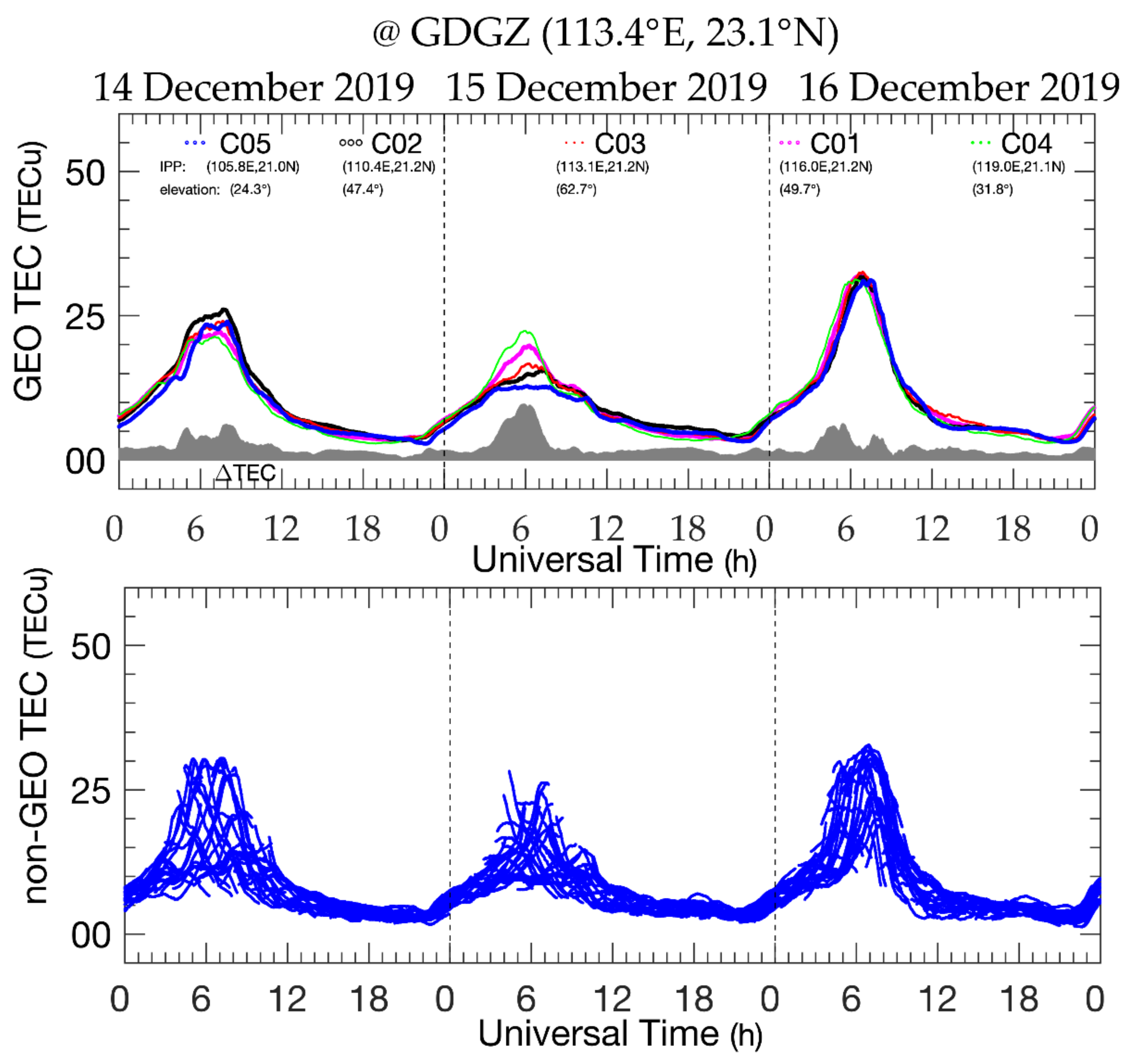
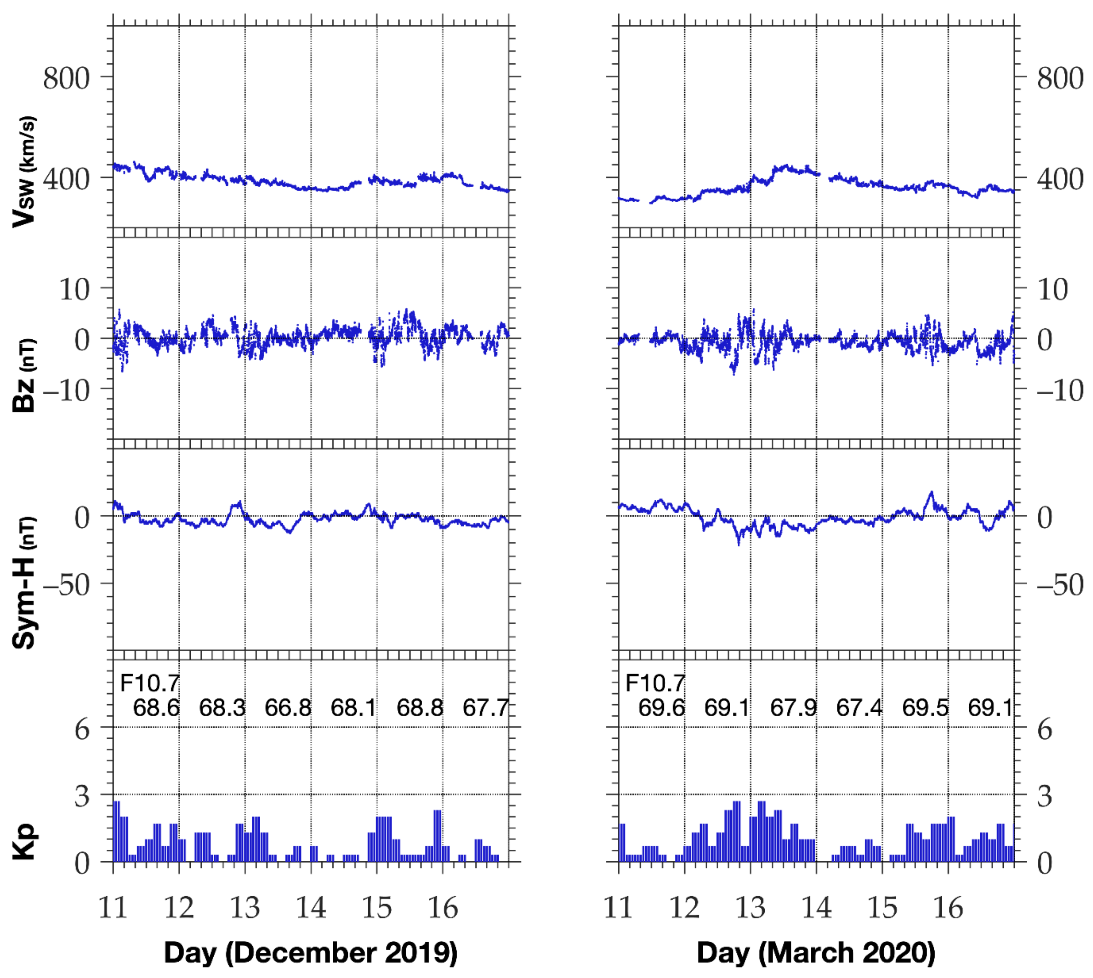
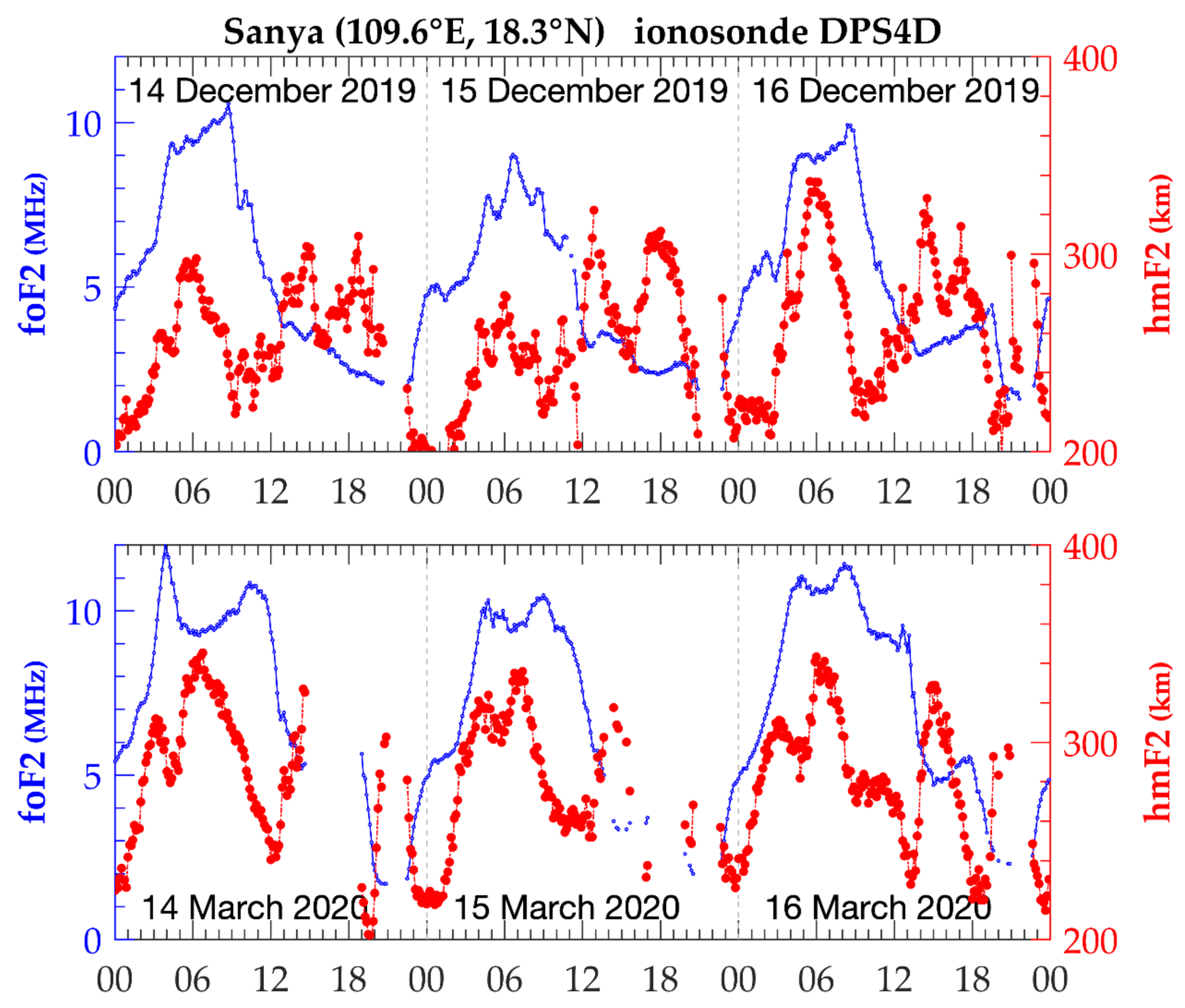
3.1.1. 14–16 December (DOY 348–350) 2019

Figure 1 plots the TEC observations recorded by the GNSS receiver GDGZ on 14–16 December 2019 (Day of Year, DOY, 348–350). We use ΔTEC to measure the absolute maximum differences among the TECs at the five GEO IPPs, which is shown as the gray area in the top panel.
The top panel of Figure 1 displays obvious day-to-day variabilities in the 3-day GEO TEC and ΔTEC detected by GDGZ. On 14 December (DOY 348) and 16 December (DOY 350) 2019, the GEO TEC had higher values and weak differences, as indicated by ΔTEC. The gray area indicates a striking feature; that is, the zonal differences of TEC grow the strongest on 15 December (DOY 349); meanwhile, the values of GEO TEC become lower, especially those of C05. The TEC values on the east side (C04) surpass those on the west side (C05) at the interval of strong longitudinal differences. Large ΔTEC persists over 3 h, peaking around 06 UT with values over 10 TECu.
Compared to the GEO TEC, the bottom panel of Figure 1 illustrates that the values of non-GEO TEC are also of vast day-to-day and spatial variabilities. The scatter in the non-GEO TEC depicts significant spatial variations of TEC in the view field of GDGZ. Although some attempts have been conducted [39,40,41,42,43], it is still a critical challenge for the community to accurately and reliably organize the spatial variations of the ionosphere from non-GEO TEC observations under the situations with large plasma density gradients. Alternatively, we prefer to use GEO TEC to examine the longitudinal pictures of the ionosphere.
Figure 2 takes a portrait of the day-to-day variabilities of TEC. The period of the data spans 37 days (DOY 329–365) in 2019. Panels in the order from top to bottom give the TEC for each of the GEO IPPs recorded by GDGZ from west to east. It can be seen from the panels of Figure 2 that there are significant day-to-day variabilities in the 37-day TEC. A quite identical pattern is displayed in the medians (blue curves) of every IPP. In contrast, the values of TEC on 15 December (DOY 349), marked by red lines, are different from the west (C05) to the east (C04). On that day, the TEC negatively deviates from medians on the west (C05 and C02), turns to close the medians (C03 and C01), and positively deviates from medians (C04).
As mentioned above, ΔTEC measures the zonal differences of the GEO TEC recorded by a GNSS receiver. The ΔTEC can be easily determined from the GEO TEC observations recorded by the GNSS network receivers. The middle point of the west GEO IPP with extremum and the east one is assigned as the weight center for a receiver. The weight center of the GEO IPPs is evaluated for each receiver for simplicity. Since the ΔTEC of GEO observations detected by GDGZ peaks around 06 UT on 15 December (Figure 1), as shown in Figure 3, the network based regional results at 06 UT on 15 December 2019. The legend labelled in the bottom-left corner of Figure 3 provides two triangles in red and blue. The size of the two triangles for the legend stands for ΔTEC with 10 TECu. A red (blue) triangle stands for the situation of TEC having a higher (lower) value on the east side than on the west side. Black points and triangles in Figure 3 give the locations of the receivers and their GEO IPPs weight centers. A larger triangle indicates a stronger longitudinal difference. It should be stressed that a triangle denotes the TEC difference being detected within a zonal range of 12° centered at its location.
It can be seen from Figure 3 that on 15 December 2019, there was a prevalence of red triangles, i.e., higher TEC on the east side than on the west at 06 UT, around the period of the peak ΔTEC detected by GDGZ. Contrary to expectations, the strong longitudinal differences appear in a narrow latitudinal band in the northern hemisphere, ranging from higher than 16°N to lower than 23°N. The big triangles have a longitude extent of about 12°, implying that the strong differences of TEC also span a narrow longitude band, ranging from around 105°E to 120°E. Interestingly, no counterpart features are found in the southern hemisphere, particularly at the two conjugate receivers. Of course, the selected GNSS receivers are very sparse over there. Out of the limited zone, the triangles are small and vary in colors (blue or red), reflecting that the longitudinal differences in TEC are much smaller.

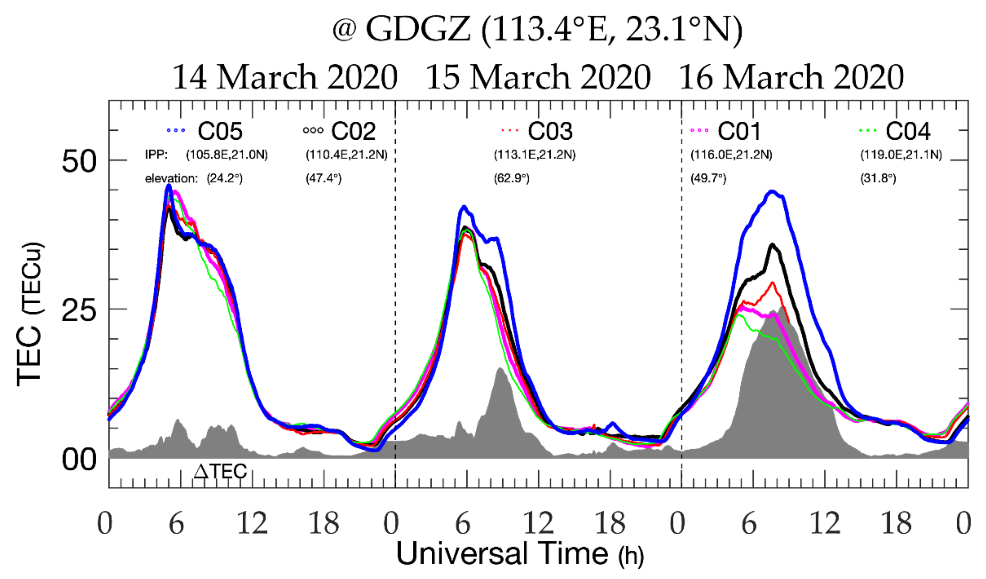
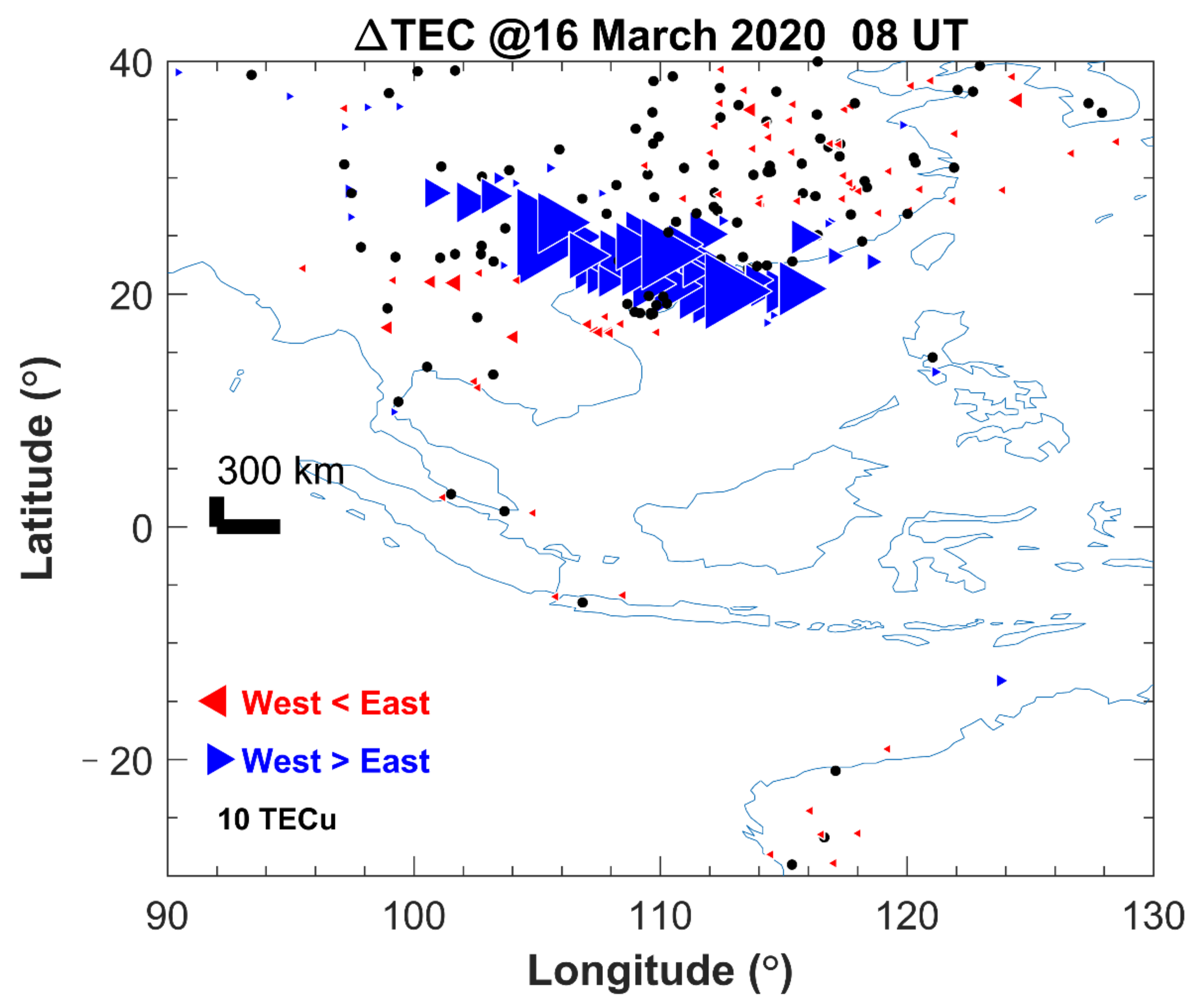
3.1.2. 14–16 March (DOY 74–76) 2020

In a similar style to Figure 1, Figure 4 shows the GEO TEC and ΔTEC recorded by GDGZ during 14–16 March (DOY 074–076) 2020. As shown in Figure 4, both GEO TEC and ΔTEC have a significant diurnal pattern and day-to-day variabilities during these three days. On 16 March (DOY 076) 2020, the ΔTEC was the largest, while the TEC of four GEO IPPs was the smallest for the three days. The ΔTEC reaches about 30 TECu at its peak time around 08–09 UT. The difference is so strong that it is comparable or even higher than the values of the TEC of C03, C01, and C04. In contrast, ΔTEC is smaller on the previous two days. The differences among GEO TEC are contributed from all IPPs, different from the pattern on the day before. On 15 March, the deviations between C05 and C02 make the absolute contribution; namely, there are many weak longitudinal differences at longitudes for the IPPs of C02-C04. Furthermore, TEC is also different in the diurnal pattern during 14–16 March 2020. Except for C04 and C01, the daytime peak of TECs at the other IPPs shifts to later hours on 16 March. Compared with Figure 1 and Figure 4, TECs of C04 are the highest on 15 December 2019, and those of C05 are the highest on 16 March 2020. ΔTEC suggests opposite longitudinal slopes on 15 December 2019 and 16 March 2020.
Figure 5 exhibits the diurnal variations of the TEC of five GEO IPPs from 25 February to 5 April (DOY 056–096) in 2020 recorded at GDGZ. It can be seen from the panels that the spread in the 41-day TEC exhibits considerable day-to-day variabilities. Similar to Figure 2, the medians (blue curves) of each IPP share a somewhat identical pattern. However, there are remarkable differences in the diurnal pattern of TEC at the five IPPs. The red lines show that the TEC deviated from the medians differently on 16 March (DOY 076). The TEC of C05 positively deviates from the medians, changes from the negative before around 07 UT to positive (C02 and C03) later, and negatively deviates from the medians (C01 and C04). In addition, the daytime peak also shifts to earlier hours for the east IPPs.
As demonstrated in Figure 4, ΔTEC at GDGZ peaks at 08–09 UT on 16 March 2020; thus, we show in Figure 6 the network based regional ΔTEC at 08 UT, in a similar style to Figure 3. The regional ΔTEC are determined from the GEO TEC observations. Big blue triangles are found to cluster in a tilted zone, ranging in latitude from higher than 18°N to lower than 30°N and longitude around 100°E to 116°E. The zone with strong west-to-east TEC differences tilts to the southeast. The extent of big triangles shows considerable longitudinal differences in a longitude range of about 95°E to 121°E. It is wider and more poleward than that in Figure 3. Similar to Figure 3, no counterpart features are found at the two receivers conjugated around the high gradient zone in the southern hemisphere. Out of the zone, the smaller size of the triangles demonstrates that the longitudinal differences in TEC are smaller and less regular.

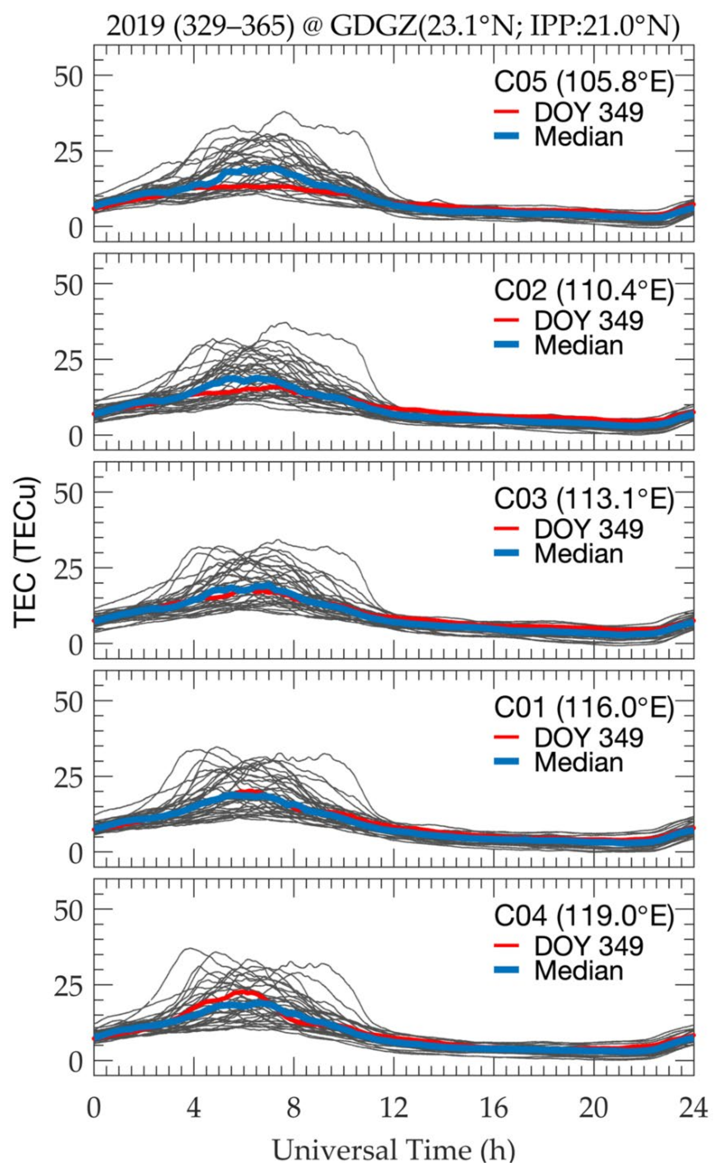
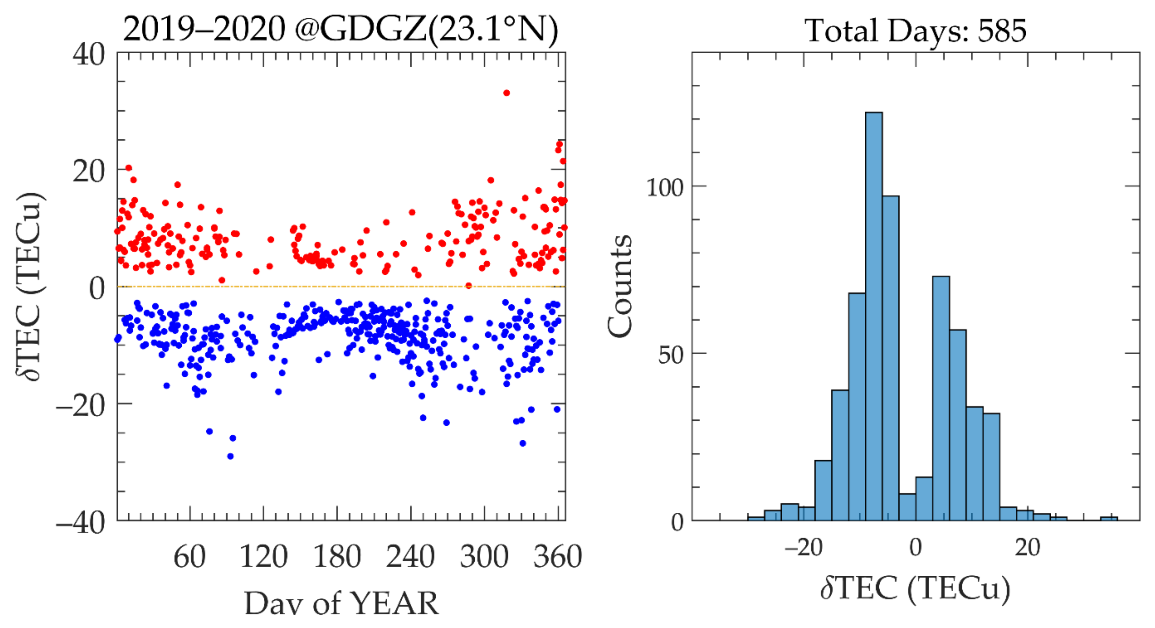
3.2. General Overview for Longitudinal Differences of TEC Recorded at GDGZ in 2019–2020

Figure 1, Figure 2, Figure 3, Figure 4, Figure 5 and Figure 6 exhibited the features of the two cases. To provide a general overview, we collect the GEO TEC observations in 2019–2020 recorded by the receiver GDGZ. The maximum and minimum of the TEC are searched every 5 min from the five GEO IPPs observations. Their corresponding IPPs or longitudes are identified simultaneously. A series of 5-min differences among the five GEO IPPs can be easily calculated from these TEC maxima and minima. Now the daily peak difference of the GEO TEC can be determined for the two years of observations at GDGZ.
We introduce δTEC to label the daily peak longitude difference. When the maximum of TEC appears at the east, δTEC has a positive value; otherwise, it will have a negative sign. The absolute value of δTEC is the ΔTEC, as described in the above subsections.
During 2019–2020, there are 585 days of observations available at GDGZ. Figure 7 depicts the histogram and the seasonal variation of δTEC in the two years. A general overview of δTEC can be drawn from Figure 7. δTEC has positive and negative signs, with somewhat dominant counts for the days of negative values. The absolute values of δTEC, or ΔTEC, vary from several TECu to tens of TECu, even higher than 20 TECu. There is a weak seasonal dependency in either δTEC or ΔTEC. In the summer season, they are smaller. Extreme values are found in the winter and equinoctial seasons.

4. Discussion

4.1. Patterns of Longitudinal Differences

The effects of the waves of lower atmospheric origins and those of the winds modulated by the global geomagnetic field configuration further contribute to the longitudinal changes in the ionosphere [8,9,10,11,12,13,14,15]. Under general circumstances, the longitudinal difference is not significant [38,41], as indicated in the patterns at GDGZ on 14 and 16 December 2019, and 14 March 2020.
Besides the generally weak differences, large longitudinal structures are occasionally present. From the two cases demonstrated in Figure 1 and Figure 4 and the general overview in 2019–2020, we can summarize the overall pattern of the longitudinal structures in TEC. They can be classified as a zonal tilt with higher values on the west side (16 March 2020 case) or with higher values on the east side (15 December 2019 case). The pattern may shift to another one, even in a single day. In addition, although strong gradients are clustered in limited regions, case studies show that they clustered at different latitude bands, not fixed. It is unclear what caused the large gradients clustered in different latitudes.
Huang et al. [23] and Liu et al. [24] also reported some strong regional gradient cases. However, there are some remarkable differences among the cases. The cases on 15 December 2019 and 16 March 2020 suggest that strong gradients may appear on the smaller TEC days, whereas the case on 11 March 2016 in Huang et al. [23] and that on 2 June 2015 in Liu et al. [24] occurred in the days of enhanced TEC values. Further, Huang et al. [23] detected cases at higher latitudes than ours.

4.2. Possible Contributors of Longitudinal Differences

It is certain that space weather, especially geomagnetic storms, may contribute vast influences to the variation and structure of the ionosphere [19,44]. Huang et al. [23] discussed the situations when geomagnetic storms occur.
Figure 8 illustrates the solar and geophysical conditions for the two cases we analyzed. The OMNI website provides information of solar 10.7 cm radio flux (F10.7), solar wind velocity (Vsw), the z component of interplanetary magnetic field (IMF Bz), and symmetrical H (Sym-H) and Kp indices during 11–16 December 2019 and 11–16 March 2020.
As shown in Figure 8, the studied periods are during solar minimum. F10.7 remains constant, with values of about 67–70 sfu (solar flux unit, 1 sfu = 1022 W/m2/Hz), indicating that the day-to-day change of solar photoionization does not involve the formation of strong longitudinal structures. As noted in the evolution of Vsw, IMF Bz, and the geomagnetic activity indices, both the solar wind and geomagnetic activity are not active on the case day and several previous days. The Kp index on the preceding days is at a level never over 3, and the Sym-H is close to zero. Therefore, the two cases exclude the contributions from solar weather. Other contributors should act as a significant agent for the strong gradients.
It is well-known that the ionosphere has distinct diurnal variations [45,46], mainly due to the evolution of the solar photoionization effect related to the Earth’s rotation. The ionosphere presents considerable and complicated diurnal pictures. Meanwhile, the local time of the east and west ionosphere is always different. Thus, one may naturally doubt that the longitudinal differences are a manifestation of the diurnal variation of the ionosphere.
To validate the local time effect, we convert the TEC shown in Figure 1 and Figure 4 as a function of universal time to the local time frame. The results are given in Figure 9. Comparing the ΔTEC in Figure 9 with Figure 1 and Figure 4, one can easily infer that the answer to the above doubt is NO. The local time effect becomes the major contributor only under circumstances when the time change rate of TEC is equal to the longitudinal change rate. However, the time change rate observed cannot meet such conditions.
Strong zonal gradients are not consistent in time and amplitude with the time change rate of TEC. It is well known that the ionosphere has distinct diurnal variation. The TEC varies mostly in sunrise and sunset hours. TEC is expected to have the largest time change rates at the sunrise and sunset hours, whereas the strong gradients grow with the values of TEC in our two cases and cases reported in Huang et al. [23] and Liu et al. [24]. Furthermore, there are strong differences in the diurnal pattern of TECs at the GEO IPPs, more remarkable than that in Hu et al. [28] and Xiong et al. [47]. The deviations of the TEC on 15 December 2019 and 16 March 2020 from the medians also provide another clue. Figure 2 and Figure 5 depict the departure from the median changes with IPPs and with cases. Strong structures may occur at times before and after the diurnal peak. All the facts support that the local time effect of the ionosphere cannot cause such intriguing and strong longitudinal structures.
Figure 10 shows the critical frequency (foF2) and peak height (hmF2) of the F2 layer observed by an ionosonde DPS4D at Sanya (109.6°E, 18.3°N) for the two cases. Sanya locates southwest of C02 IPP of GDGZ. Sanya locates about 330 km away from C02 IPP but within the zone of the intense gradients (see Figure 2 and Figure 5). The foF2 observations at Sanya share a roughly similar day-to-day variability with C02 TEC at GDGZ. The hmF2 at Sanya can indicate the day-to-day changes of dynamical processes in the equatorial and low-latitude ionosphere. As seen from Figure 10, hmF2 has lower values at the intervals of strong longitudinal structures around 06 UT on 15 December 2019 and 08 UT on 16 March 2020, compared to the other two days. The lower hmF2 is more evident for the 15 December 2019 case.
The equatorial zonal electric field or vertical plasma drift is the dominant dynamical factor controlling the equatorial and low-latitude ionosphere [48,49]. We use the equatorial electrojet (EEJ), indicated by the intensity of ΔH, to infer the equatorial zonal electric field changes, according to their close relationship [48]. ΔH is determined from the difference of the observations of H, the horizontal magnetic field component, recorded by an equatorial magnetometer at Da Lat (108.4°E, 11.9°N) and by an off-equatorial magnetometer at Phu Thuy (106.0°E, 21.0°N). The two magnetometers locate quite close to the longitude of the westmost GEO IPP C05 of the receiver GDGZ.
Figure 11 gives the estimated ΔH during 14–16 December 2019 and 14–16 March 2020. From Figure 11, we can see that both the daily intensity and peak time of EEJ change day by day. For the December 2019 case, the EEJ values on 15 December lie between the other two days during the persistence of strong gradients. Meanwhile, for the March 2020 case, the EEJ has higher values at the strong difference times.
Liu et al. [24] also investigated the EEJ behavior in the course of strong gradients. They found that both the intensity of EEJ and TEC values over the gradient region share a consistent day-to-day pattern. On 1–2 June 2015, when ΔTEC becomes the strongest among the several days, the enhancements of TEC are most significant, and the EEJ also registers the maximum compared to the previous days. The enhancement in TEC over the EIA crest region is widely considered a manifestation of an intensified electric field [24,49].
However, for the current two cases, during the strong zonal gradients, there are smaller values of hmF2 at Sanya, while the EEJ has discrepant performances between the cases.
Most importantly, there is a hemispheric asymmetry of the strong longitudinal difference. We choose two cases in different seasons, one in the northern winter and another one in the vernal equinox. As illustrated in Figure 3 and Figure 6, no strong differences are present in the longitudinal TEC in the southern hemisphere. The absence in the southern hemisphere highlights that the equatorial electric field may not be the most important agent responsible for forming strong longitude structures. Otherwise, strong differences should be present in the southern hemisphere. At the very least, some other drivers are expected to be involved in forming such interesting phenomena.

4.3. Performance of GIMs

Figure 12 and Figure 13 display some snapshots of the TEC at 20°N in the Asian sector as a function of longitudes. Snapshots are taken at 00, 02, 04, 06, 07, and 09 UT for the 15 December 2019 case, and at 02, 04, 06, 08, 10, and 12 UT for the 16 March 2020 case, respectively, corresponding to the times before, during, and after the strong gradients. The TEC is from our regional GNSS observations and those of CODE and MIT TEC. The black dots for the regional observed TEC show clearly that the strong structure around 20°N should not be a part of the normal long scale longitude structures [15,16,17,18]. This is more visible at 06 and 07 UT on 15 December 2019.
We choose the GIM TEC products provided by CODE and MIT to demonstrate the performance of GIM TEC under the studied circumstances. From the snapshots, we can see that the TEC products perform relatively well and are comparable at times without strong structures, although there are some differences in the values. In general, MIT TEC has a stronger ability to capture the longitudinal variations of the regional TEC. Compared to CODE GIMs, the MIT products have a more reliable presentation.
It has been reported that the GIM TEC products can describe the wave-like structures in the low-latitude ionosphere [17,50]. Currently, many GIMs take a spatial resolution of 5° in longitude and 2.5° in latitude [36], and MIT products have a spatial resolution of 1°. It is expected that a finer spatial resolution may provide more accurate pictures of the global ionosphere when the GNSS receivers are reasonably distributed worldwide. However, the GNSS receivers used in the GIMs are relatively sparse in some regions. Thus, international cooperation is calling for improving the ability to describe the structures of the ionosphere.
In addition, it should be cautioned that we must realize the possible degradation of the reliability of some ionospheric observations when there are strong zonal gradients. Unfortunately, our attention is generally focused on the impact of latitudinal structures [2,39].

5. Conclusions

In this work, we investigated the regional longitudinal differences in the low latitude ionosphere. The GNSS TEC observations in the Asian-Australian sector provide new findings, as summarized below.
(1)
The GNSS TEC observations in 2019–2020 exhibit diverse longitudinal structures in the northern low-latitude ionosphere. Intense zonal differences may occur with highest TEC on the east or west side, regardless of geomagnetic activity conditions.
(2)
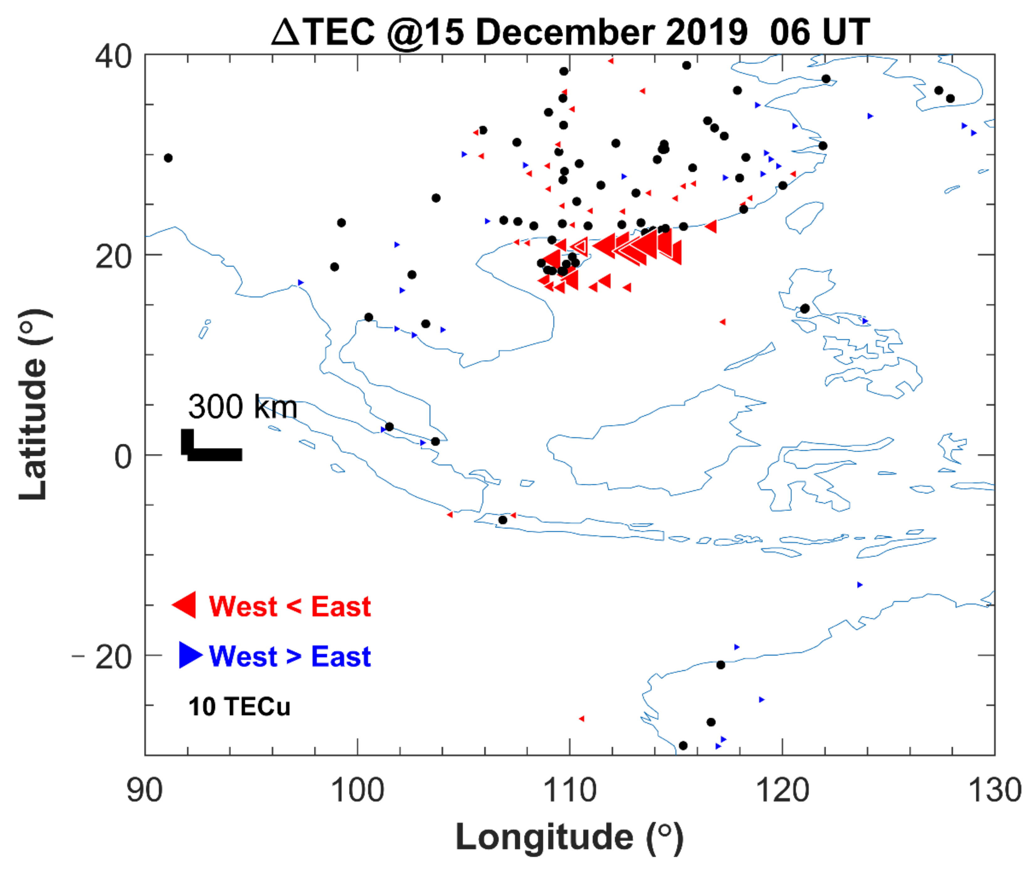
The strong zonal differences are clustered in a narrow zone. The zone is different case by case. The spatial extent of this phenomenon highlights that it is a new kind of spatial structure, not the extreme presentation of the large-scale longitudinal variations reported before.
(3)
There are evident and diverse zonal differences in the departures from the medians during the period of strong gradients. The features of the strong differences cannot be satisfactorily explained in terms of the local time effects of the diurnal variations of the ionosphere.
(4)
Strong zonal differences are absent in the conjugated region in the southern hemisphere in the two cases.
(5)
The regional scale longitudinal structures with strong differences challenge the presentation of the current GIMs. It suggests a finer spatial resolution being adopted in future products of GIMs.

Author Contributions

Conceptualization, L.L.; Data curation, Y.Y., G.L. and W.S.; Formal analysis, L.L. and Y.Y.; Methodology, L.L. and Y.Y.; Validation, R.Z., Y.C., H.L. and H.Z.; Writing—original draft, L.L. and Y.Y.; Writing—review & editing, L.L., Y.C., H.L. and H.Z. All authors have read and agreed to the published version of the manuscript.

Funding

This research was supported by National Natural Science Foundation of China (42030202), National key research and development program (2017YFE0131400), and the Open Research Project of Large Research Infrastructures of CAS-”Study on the interaction between low/mid-latitude atmosphere and ionosphere based on the Chinese Meridian Project”.

Data Availability Statement

The Meridian Project of China provided funding in the ionosonde chain. The data of ionosonde observations and the GNSS rinex files are archived from World Data Center for Geophysics, Beijing (http://www.geophys.ac.cn/, last accessed 25 March 2022). Other GNSS data are requested from the Crustal Movement Observation Network of China (CMONOC) and downloaded from IGS FTP site (ftp://gdc.cddis.eosdis.nasa.gov/, last accessed on 25 March 2022). The CODE GIM data can be accessed from the FTP side (ftp://igs.ensg.eu//pub/igs/products/ionosphere/, last accessed on 25 March 2022). The Haystack Observatory of Massachusetts Institute of Technology provided TEC data products, which can be accessed through the Madrigal distributed data system (http://www.openmadrigal.org/, last accessed on 2 March 2022). The data of daily solar flux and 1-min averaged solar wind, SYM-H, and Kp indices are downloaded from the OMNI database, which are available at https://omniweb.gsfc.nasa.gov/ (last accessed on 25 March 2022). The data of magnetometers are provided from the site (https://www.intermagnet.org/, last accessed on 25 March 2022).

Acknowledgments

The authors appreciate Xiukuang Zhao for providing the GNSS data. They also acknowledge the use of data from the Crustal Movement Observation Network of China (CMONOC) and the Chinese Meridian Project.

Conflicts of Interest

The authors declare no conflict of interest.

References

  1. Schaer, S. Mapping and Predicting the Earths Ionosphere using the Global Positioning System. Ph.D. Thesis, University of Bern, Bern, Switzerland, 1999. [Google Scholar]
  2. Yue, X.; Schreiner, W.S.; Lei, J.; Sokolovskiy, S.V.; Rocken, C.; Hunt, D.C.; Kuo, Y.-H. Error analysis of Abel retrieved electron density profiles from radio occultation measurements. Ann. Geophys. 2010, 28, 217–222. [Google Scholar] [CrossRef] [Green Version]
  3. Yang, Y.; Liu, L.; Zhao, X.; Xie, H.; Chen, Y.; Le, H.; Zhang, R.; Tariq, M.A.; Li, W. Ionospheric Nighttime Enhancements at Low Latitudes Challenge Performance of the Global Ionospheric Maps. Remote Sens. 2022, 14, 1088. [Google Scholar] [CrossRef]
  4. Liu, L.; Chen, Y.; Le, H.; Ning, B.; Wan, W.; Liu, J.; Hu, L. A case study of postmidnight enhancement in F-layer electron density over Sanya of China. J. Geophys. Res. Space Phys. 2013, 118, 4640–4648. [Google Scholar] [CrossRef]
  5. Li, Z.; Wang, N.; Li, M.; Zhou, K.; Yuan, Y.B.; Yuan, H. Evaluation and analysis of the global ionospheric TEC map in the frame of international GNSS services. Chin. J. Geophys. 2017, 60, 3718–3729. [Google Scholar] [CrossRef]
  6. Liu, L.; Le, H.; Wan, W.; Sulzer, M.P.; Lei, J.; Zhang, M.-L. An analysis of the scale heights in the lower topside ionosphere based on the Arecibo incoherent scatter radar measurements. J. Geophys. Res. Space Phys. 2007, 112, A06307. [Google Scholar] [CrossRef] [Green Version]
  7. Heelis, R.A.; Coley, W.R. Variations in the low- and middle-latitude topside ion concentration observed by DMSP during superstorm events. J. Geophys. Res. 2007, 112, A08310. [Google Scholar] [CrossRef] [Green Version]
  8. Zhang, S.-R.; Foster, J.C.; Coster, A.J.; Erickson, P.J. East-West Coast differences in total electron content over the continental US. Geophys. Res. Lett. 2011, 38, L19101. [Google Scholar] [CrossRef] [Green Version]
  9. Zhang, S.-R.; Foster, J.C.; Holt, J.M.; Erickson, P.J.; Coster, A.J. Magnetic declination and zonal wind effects on longitudinal differences of ionospheric electron density at midlatitudes. J. Geophys. Res. Space Phys. 2012, 117, A08329. [Google Scholar] [CrossRef] [Green Version]
  10. Zhao, B.; Wang, M.; Wang, Y.; Ren, Z.; Yue, X.; Zhu, J.; Wan, W.; Ning, B.; Liu, J.; Xiong, B. East-west differences in F-region electron density at midlatitude: Evidence from the Far East region. J. Geophys. Res. Space Phys. 2013, 118, 542–553. [Google Scholar] [CrossRef]
  11. Xu, J.S.; Li, X.J.; Liu, Y.W.; Jing, M. TEC differences for the mid-latitude ionosphere in both sides of the longitudes with zero declination. Adv. Space Res. 2014, 54, 883–895. [Google Scholar] [CrossRef]
  12. Li, Q.; Liu, L.; Balan, N.; Huang, H.; Zhang, R.; Chen, Y.; Le, H. Longitudinal structure of the midlatitude ionosphere using COSMIC electron density profiles. J. Geophys. Res. Space Phys. 2018, 123, 8766–8777. [Google Scholar] [CrossRef]
  13. Xiong, C.; Lühr, H. The Midlatitude Summer Night Anomaly as observed by CHAMP and GRACE: Interpreted as tidal features. J. Geophys. Res. Space Phys. 2014, 119, 4905–4915. [Google Scholar] [CrossRef] [Green Version]
  14. Ma, H.; Liu, L.; Chen, Y.; Le, H.; Li, Q.; Zhang, H. Longitudinal differences in electron temperature on both sides of zero declination line in the mid-latitude topside ionosphere. J. Geophys. Res. Space Phys. 2021, 126, e2020JA028471. [Google Scholar] [CrossRef]
  15. Immel, T.J.; Sagawa, E.; England, S.L.; Henderson, S.B.; Hagan, M.E.; Mende, S.B.; Frey, H.U.; Swenson, C.M.; Paxton, L.J. Control of equatorial ionospheric morphology by atmospheric tides. Geophys. Res. Lett. 2006, 33, L15108. [Google Scholar] [CrossRef]
  16. Kil, H.; Lee, W.K.; Kwak, Y.-S.; Oh, S.-J.; Paxton, L.J.; Zhang, Y. Persistent longitudinal features in the low-latitude ionosphere. J. Geophys. Res. 2012, 117, A06315. [Google Scholar] [CrossRef] [Green Version]
  17. Wan, W.; Liu, L.; Pi, X.; Zhang, M.-L.; Ning, B.; Xiong, J.; Ding, F. Wavenumber-4 patterns of the total electron content over the low latitude ionosphere. Geophys. Res. Lett. 2008, 35, L12104. [Google Scholar] [CrossRef]
  18. Ren, Z.; Wan, W.; Liu, L.; Zhao, B.; Wei, Y.; Yue, X.; Heelis, R.A. Longitudinal variations of electron temperature and total ion density in the sunset equatorial topside ionosphere. Geophys. Res. Lett. 2008, 35, L05108. [Google Scholar] [CrossRef] [Green Version]
  19. Mendillo, M. Storms in the ionosphere: Patterns and processes for total electron content. Rev. Geophys. 2006, 44, RG4001. [Google Scholar] [CrossRef]
  20. Fagundes, P.R.; Cardoso, F.A.; Fejer, B.G.; Venkatesh, K.; Ribeiro, B.A.G.; Pillat, V.G. Positive and negative GPS-TEC ionospheric storm effects during the extreme space weather event of March 2015 over the Brazilian sector. J. Geophys. Res. Space Phys. 2016, 121, 5613–5625. [Google Scholar] [CrossRef] [Green Version]
  21. Liu, L.; Le, H.; Chen, Y.; Zhang, R.; Wan, W. New Aspects of the ionospheric behavior over Millstone Hill during the 30-day incoherent scatter radar experiment in October 2002. J. Geophys. Res. Space Phys. 2019, 124, 6288–6295. [Google Scholar] [CrossRef]
  22. Kuai, J.; Liu, L.; Liu, J.; Sripathi, S.; Zhao, B.; Chen, Y.; Le, H.; Hu, L. Effects of disturbed electric fields in the low-latitude and equatorial ionosphere during the 2015 St. Patrick’s Day storm. J. Geophys. Res. Space Phys. 2016, 121, 9111–9126. [Google Scholar] [CrossRef]
  23. Huang, F.; Lei, J.; Dou, X. Daytime ionospheric longitudinal gradients seen in the observations from a regional BeiDou GEO receiver network. J. Geophys. Res. Space Phys. 2017, 122, 6552–6561. [Google Scholar] [CrossRef]
  24. Liu, L.; Ding, Z.; Zhang, R.; Chen, Y.; Le, H.; Zhang, H.; Wu, J.; Wan, W. A case study of the enhancements in ionospheric electron density and its longitudinal gradient at Chinese low latitudes. J. Geophys. Res. Space Phys. 2020, 125, e2019JA027751. [Google Scholar] [CrossRef]
  25. Sunda, S.; Vyas, B.M. Local time, seasonal, and solar cycle dependency of longitudinal variations of TEC along the crest of EIA over India. J. Geophys. Res. Space Phys. 2013, 118, 6777–6785. [Google Scholar] [CrossRef]
  26. Vladimer, J.A.; Jastrzebski, P.; Lee, M.C.; Doherty, P.H.; Decker, D.T.; Anderson, D.N. Longitude structure of ionospheric total electron content at low latitudes measured by the TOPEX/Poseidon satellite. Radio Sci. 1999, 34, 1239–1260. [Google Scholar] [CrossRef] [Green Version]
  27. Sun, W.; Wu, B.; Wu, Z.; Hu, L.; Zhao, X.; Zheng, J.; Xie, H.; Yang, S.; Ning, B.; Li, G. IONISE: An ionospheric observational network for irregularity and scintillation in East and Southeast Asia. J. Geophys. Res. Space Phys. 2020, 125, e2020JA028055. [Google Scholar] [CrossRef]
  28. Hu, L.; Yue, X.; Ning, B. Development of the Beidou Ionospheric Observation Network in China for space weather monitoring. Space Weather 2017, 15, 974–984. [Google Scholar] [CrossRef]
  29. Yuan, Y.; Li, Z.; Wang, N.; Zhang, B.; Li, H.; Li, M.; Huo, X.; Ou, J. Monitoring the ionosphere based on the Crustal Movement Observation Network of China. Geod. Geodyn. 2015, 16, 73–80. [Google Scholar] [CrossRef] [Green Version]
  30. Aa, E.; Huang, W.; Yu, S.; Liu, S.; Shi, L.; Gong, J.; Chen, Y.; Shen, H. A regional ionospheric TEC mapping technique over China and adjacent areas on the basis of data assimilation. J. Geophys. Res. Space Phys. 2015, 120, 5049–5061. [Google Scholar] [CrossRef] [Green Version]
  31. She, C.; Yue, X.; Hu, L.; Zhang, F. Estimation of Ionospheric Total Electron Content from a Multi-GNSS Station in China. IEEE Trans. Geosci. Remote Sens. 2020, 58, 852–860. [Google Scholar] [CrossRef]
  32. Prol, F.D.S.; Camargo, P.D.O.; Monico, J.F.G.; Muella, D.A.H. Assessment of a TEC calibration procedure by single-frequency PPP. GPS Solut. 2018, 22, 35. [Google Scholar] [CrossRef] [Green Version]
  33. Rideout, W.; Coster, A. Automated GPS processing for global total electron content data. GPS Solut. 2006, 10, 219–228. [Google Scholar] [CrossRef]
  34. Mannucci, A.; Wilson, B.; Yuan, D.; Ho, C.; Lindqwister, U.; Runge, T. A global mapping technique for GPS-derived ionospheric total electron content measurements. Radio Sci. 1998, 33, 565–582. [Google Scholar] [CrossRef]
  35. Roma-Dollase, D.; Hernández-Pajares, M.; Krankowski, A.; Kotulak, K.; Ghoddousi-Fard, R.; Yuan, Y.; Li, Z.; Zhang, H.; Shi, C.; Wang, C.; et al. Consistency of seven different GNSS global ionospheric mapping techniques during one solar cycle. J. Geod. 2018, 92, 691–706. [Google Scholar] [CrossRef] [Green Version]
  36. Li, Z.; Wang, N.; Liu, A.; Yuan, Y.; Wang, L.; Hernández-Pajares, M.; Krankowski, A.; Yuan, H. Status of CAS global ionospheric maps after the maximum of solar cycle 24. Satell. Navig. 2021, 2, 19. [Google Scholar] [CrossRef]
  37. Komjathy, A.; Sparks, L.; Wilson, B.D.; Mannucci, A.J. Automated daily processing of more than 1000 ground-based GPS receivers for studying intense ionospheric storms. Radio Sci. 2005, 40, RS6006. [Google Scholar] [CrossRef] [Green Version]
  38. Hernandez-Pajares, M.; Juan, J.; Sanz, J. New approaches in global ionospheric determination using ground gps data. J. Atmos. Sol. Terr. Phys. 1999, 61, 1237–1247. [Google Scholar] [CrossRef]
  39. Nava, B.; Radicella, S.M.; Leitinger, R.; Coisson, P. Use of total electron content data to analyze ionosphere electron density gradients. Adv. Space Res. 2007, 39, 1292–1297. [Google Scholar] [CrossRef]
  40. Kim, J.; Lee, S.W.; Lee, H.K. An annual variation analysis of the ionospheric spatial gradient over a regional area for GNSS applications. Adv. Space Res. 2014, 54, 333–341. [Google Scholar] [CrossRef]
  41. Jakowski, N.; Stankov, S.M.; Schlueter, S.; Klaehn, D. On developing a new ionospheric perturbation index for space weather operations. Adv. Space Res. 2006, 38, 2596–2600. [Google Scholar] [CrossRef]
  42. Juan, J.M.; Sanz, J.; Rovira-Garcia, A.; González-Casado, G.; Ibáñez, D.; Perez, R.O. AATR an ionospheric activity indicator specifically based on GNSS measurements. J. Space Weather Space Clim. 2018, 8, A14. [Google Scholar] [CrossRef]
  43. Srinivas, V.S.; Sarma, A.D.; Reddy, A.S.; Reddy, D.K. Investigation of the Effect of Ionospheric Gradients on GPS Signals in the Context of LAAS. Prog. Electromagn. Res. B 2014, 57, 191–205. [Google Scholar] [CrossRef] [Green Version]
  44. Heelis, R.A.; Maute, A. Challenges to Understanding the Earth’s Ionosphere and Thermosphere. J. Geophys. Res. Space Phys. 2020, 125, e2019JA027497. [Google Scholar] [CrossRef]
  45. Klobuchar, J.A. Ionospheric time-delay algorithm for single-frequency GPS users. IEEE Trans. Aerosp. Electron. Syst. 1987, AES-23, 325–331. [Google Scholar] [CrossRef]
  46. Liu, L.B.; Chen, Y.D.; Zhang, R.L.; Le, H.J.; Zhang, H. Some investigations of ionospheric diurnal variation. Rev. Geophys. Planet. Phys. 2021, 52, 647–661. [Google Scholar] [CrossRef]
  47. Xiong, B.; Wan, W.; Yu, Y.; Hu, L. Investigation of ionospheric TEC over China based on GNSS data. Adv. Space Res. 2016, 58, 867–877. [Google Scholar] [CrossRef]
  48. Anderson, D.; Anghel, A.; Yumoto, K.; Ishitsuka, M.; Kudeki, E. Estimating daytime vertical ExB drift velocities in the equatorial F-region using ground-based magnetometer observations. Geophys. Res. Lett. 2002, 29, 1596. [Google Scholar] [CrossRef]
  49. Zhao, B.; Wan, W.; Liu, L.; Igarashi, K.; Nakamura, M.; Paxton, L.J.; Su, S.-Y.; Li, G.; Ren, Z. Anomalous enhancement of ionospheric electron content in the Asian-Australian region during a geomagnetically quiet day. J. Geophys. Res. 2008, 113, A11302. [Google Scholar] [CrossRef] [Green Version]
  50. Mukhtarov, P.; Pancheva, D.; Andonov, B.; Pashova, L. Global TEC maps based on GNSS data: 1. Empirical background TEC model. J. Geophys. Res. Space Phys. 2013, 118, 4594–4608. [Google Scholar] [CrossRef]
Figure 1. Temporal evolution of the TEC observations from the GNSS receiver GDGZ (113.4°E, 23.1°N) on 14–16 December 2019 (day of year (DOY) 348–350). The bottom panel plots the non-GEO TEC. The top panel is for the GEO observations. The TEC of the five GEO PRNs, along with their elevation angles and IPPs coordinates, are labelled. Gray shaded area plots ΔTEC, the peak difference of the GEO TECs covering longitudes from 105.8°E to 119.0°E.
Remotesensing 14 02315 g001
Figure 2. The daily GEO TEC recorded at GDGZ during DOY 329–365 in 2019. In each panel the red curve marks the data of each of the IPPs on 15 December (DOY 349), and the blue line plots the medians during the period.
Remotesensing 14 02315 g002
Figure 3. Distribution of the network-based ΔTEC strength at 06 UT on 15 December (DOY 349) in 2019. Red (blue) triangles denote higher TEC on the east (west) side. The black points mark the locations of GNSS receivers. The solid horizontal and vertical bars around the equator are scales measuring a distance of 300 km in the zonal and meridional directions, respectively. The red and blue triangles at the bottom left corner act as a scale of 10 TECu.
Remotesensing 14 02315 g003
Figure 4. Similar to Figure 1, but for the GEO TEC and ΔTEC during 14–16 March (DOY 074–076) 2020.
Remotesensing 14 02315 g004
Figure 5. Similar to Figure 2, but for those during DOY 056–096 in 2020. The red curves mark the data of GEO IPPs on 16 March (DOY 076), and the blue lines plot the medians during the period.
Remotesensing 14 02315 g005
Figure 6. Similar to Figure 2, but for the case at 08 UT on 16 March (DOY 076) 2020.
Remotesensing 14 02315 g006
Figure 7. Seasonal variation and the histogram of δTEC, the daily peak longitudinal difference of GEO TEC.
Remotesensing 14 02315 g007
Figure 8. Solar 10.7 cm radio flux (F10.7), solar wind velocity (Vsw), interplanetary magnetic field z component (Bz), and symmetrical H (Sym-H) and Kp indices during 11–16 December 2019 and 11–16 March 2020.
Remotesensing 14 02315 g008
Figure 9. Local time variation of the TEC of the five GEO IPPs recorded at GDGZ on 15 December 2019 and 16 March 2020.
Remotesensing 14 02315 g009
Figure 10. The critical frequency (foF2) and peak height (hmF2) of the F2 layer observed by Sanya DPS4D ionosonde during 14–16 December 2019 and 14–16 March 2020, respectively.
Remotesensing 14 02315 g010
Figure 11. The equatorial electrojet (EEJ) during 14–16 December 2019 and 14–16 March 2020. The EEJ is indicated by ΔH, the intensity difference of the horizontal magnetic field component recorded at Da Lat, an equatorial magnetometer, and at Phu Thuy, an off-equatorial magnetometer.
Remotesensing 14 02315 g011
Figure 12. Snapshots of the longitudinal variation of the TEC from the network of GNSS receivers, CODE GIM, and MIT TEC products on 15 December 2019. The black dots are the regional GNSS TEC observations, the green pluses are for that of MIT TEC, and the brown curves for the CODE TEC.
Remotesensing 14 02315 g012
Figure 13. Same as Figure 12, but for the case on 16 March 2020.
Remotesensing 14 02315 g013
Publisher’s Note: MDPI stays neutral with regard to jurisdictional claims in published maps and institutional affiliations.

