Article

A Method for Classifying Complex Features in Urban Areas Using Video Satellite Remote Sensing Data

1
School of Resource and Environmental Sciences, Wuhan University, Wuhan 430079, China
2
Land Satellite Remote Sensing Application Center, Ministry of Natural Resources of P.R. China, Beijing 100048, China
3
The State Key Laboratory of Information Engineering in Surveying, Mapping and Remote Sensing (LIESMARS), Wuhan University, Wuhan 430079, China
4
Collaborative Innovation Center of Geospatial Technology, Wuhan 430079, China
5
Ecology and Environment Monitoring and Scientific Research Center, Yangtze Basin Ecology and Environment Administration, Ministry of Ecology and Environment of the P.R. China, Wuhan 430014, China
*
Author to whom correspondence should be addressed.
Remote Sens. 2022, 14(10), 2324; https://doi.org/10.3390/rs14102324
Submission received: 23 March 2022 / Revised: 4 May 2022 / Accepted: 6 May 2022 / Published: 11 May 2022

Abstract

:
The classification of optical satellite-derived remote sensing images is an important satellite remote sensing application. Due to the wide variety of artificial features and complex ground situations in urban areas, the classification of complex urban features has always been a focus of and challenge in the field of remote sensing image classification. Given the limited information that can be obtained from traditional optical satellite-derived remote sensing data of a classification area, it is difficult to classify artificial features in detail at the pixel level. With the development of technologies, such as satellite platforms and sensors, the data types acquired by remote sensing satellites have evolved from static images to dynamic videos. Compared with traditional satellite-derived images, satellite-derived videos contain increased ground object reflection information, especially information obtained from different observation angles, and can thus provide more information for classifying complex urban features and improving the corresponding classification accuracies. In this paper, first, we analyze urban-area, ground feature characteristics and satellite-derived video remote sensing data. Second, according to these characteristics, we design a pixel-level classification method based on the application of machine learning techniques to video remote sensing data that represents complex, urban-area ground features. Last, we conduct experiments on real data. The test results show that applying the method designed in this paper to classify dynamic, satellite-derived video remote sensing data can improve the classification accuracy of complex features in urban areas compared with the classification results obtained using static, satellite-derived remote sensing image data at the same resolution.

1. Introduction

The classification of remote sensing images derived from optical satellites is an important application in the field of satellite remote sensing. As the resolution of satellite-derived remote sensing imagery has gradually improved, research goals have progressively developed from classifying objects of several kilometers to classifying objects of several meters. In terms of object categorization, research has also developed from classifying natural features to delineating artificial features. However, many types of artificial ground features exist in urban areas, and the reflection characteristics of these features can be relatively similar. The pixel spectra reflected in traditional static, multispectral remote sensing data can be applied to better classify certain artificial ground feature categories. However, these traditional data present certain challenges with regard to the classification of certain artificial feature categories, such as commercial areas, residential areas and cement squares, all of which are artificial structures.
Scholars, practitioners and professionals worldwide have begun to use multiangle, ground feature reflection information to distinguish different types of ground features. A two-stage framework to extract spatial and motion features from satellite video scenes to perform feature classification was proposed in [1,2]. Research to revealing events of interest (EOIs) from satellite video scenes using a two-stream method was devoted in [3]. Satellite video data to perform spatiotemporal scene interpretations were processed in [4].
Aiming to classify multiangle optical remote sensing images with a focus on the classification of natural features, remote sensing data collected by the Ziyuan (ZY-3) satellite at three observation angles were classified in [5]. The remote sensing data recorded by the multiangle imaging spectroradiometer (MISR) aboard the Earth Observing System (EOS) Terra satellite at 9 observation angles were classified in [6,7]. The weighted super-resolution reconstruction method for multiangle remote sensing images was adapted to alleviate the limitations associated with the use of images with different resolutions in [8]. An improved land cover classification study based on fusion data derived from multiple sources and multitemporal satellite data, including data from the Gaofen (GF-1) satellite and moderate resolution imaging spectroradiometer (MODIS) normalized difference vegetation index (NDVI) data were conducted in [9,10]. A bidirectional reflectance factor (BRF) product was developed using the multiangle implementation of the atmospheric correction (MAIAC) algorithm by the MODIS science team in [11]. A sensor design and methodology for the direct retrieval of forest light use efficiency (LUE) changes from space were suggested by measuring the photochemical reflectance index (PRI) of the shadow fraction with a multiangle spectrometer in [12]. Regarding the classification of complex features, a remote sensing classification study of local climate zones in high-density cities and a simultaneous road-extraction method for complex urban areas by incorporating very-high-resolution images were presented by [13,14]. Moreover, in a geometric potential assessment experiment performed on ZY3-02 triple-linear-array imagery, several variation types were determined, such as changes in the thermal environment, which can alter the installation angle of the camera, thus leading to varying geometric performances in [15].
A few studies and experiments have been conducted with a focus on satellite-derived video remote sensing data. An on-orbit relative radiometric calibration method for optical video satellites was proposed to address the high-frame-rate characteristics of video satellites in [16]. Regarding the classification of moving targets and events, point-target tracking for satellite video data based on the Hu correlation filter, the ship detection and tracking method based on multiscale saliency and contrast analysis in the surrounding region to enhance the defined recall and precision abilities of satellite video data were carried out in [17,18]. The motion detection sensitivity of instant learning algorithms applied to satellite-derived videos for weather forecasting was enhanced in [19]. In addition, an ingenious method for processing big surveillance video data acquired from smart monitoring cameras was developed in [20].
These past experiments showed that remote sensing data obtained from multiple angles contain more abundant information than single-angle data and can thus provide a basis for an increasingly accurate ground feature classification method and a novel approach to ground feature recognition and classification research. The purpose of this paper is to obtain a method for classifying video satellite remote sensing data that requires less computation than traditional methods. Compared with static, satellite remote sensing image data, video satellite data with the method in this paper can obtain higher classification accuracy. A method for classifying video satellite remote sensing data, which requires less computation than traditional methods, is designed. A variety of parameters of input data are employed during the experiment.

2. Materials and Methods

2.1. Data Sources

The satellite-derived video data utilized in this study were obtained from the Jilin-1 agile video satellite constructed by Chang Guang Satellite Technology Co., Ltd. in Jinlin, China. Different from traditional Earth observation satellites, this satellite can obtain high-resolution, 3-band, color video data of the same scene for a maximum duration of 120 s with 25 frames per second. The ground resolution of each pixel at the nadir point can reach 1.13 m. The resulting imagery contains 3 bands: red band, green band, and blue band. The Jilin-1 agile video satellite has the ability to obtain hundreds of uncompressed, continuous, multiple-observation-angle images instead of the highly compressed video data reflected by the H.264, H.265 and MP4 standards. Thus, this satellite can generate and retain much more information than traditional methods while simultaneously increasing the data volume.
As an experiment, we selected a 600 × 950-pixel area that contains a rich variety of land cover types from the satellite-derived video dataset; an image from this dataset is shown in Figure 1a.
The characteristics of the utilized experimental data are briefly described as follows:
  • City represented by the video satellite remote sensing data: New Delhi, India;
  • Size of the data: 600 × 950 pixels;
  • Ground resolution of the data: approximately 1.13 m;
  • Bandwidths of the data: blue band, 437–512 nm; green band, 489–585 nm; and red band: 580–723 nm;
  • Dynamic range of the data: 8 bits (0–255) for each channel;
  • Data acquisition duration: 28 s; number of observation angles (frames): 700.
Regarding the ground-truth data, first, we obtained a high-resolution image of the study location from Google Earth, as shown in Figure 1b; second, we used both the video satellite and Google Earth data sources to select ground-truth data corresponding to different land cover types. We manually selected 8 significantly different land cover classes/types according to the two datasets.
In our experiment, the 8 selected land classes included grasslands, trees, bare soils, factory district buildings, residential district buildings, business district buildings, asphalt roads, and concrete roads. The number of pixels corresponding to each land cover class ranged from 335 to 6715 which are listed in Table 1. A color image of the video satellite data and a labeled map showing the eight ground-truth land cover classes are shown in Figure 1c.
Among the 8 selected feature types, residential buildings, factory buildings and business buildings are architecture types, while concrete roads and most building tops are cement materials. Due to the similar characteristics of these features, it is difficult to accurately distinguish them using traditional remote sensing image data. This has always been a difficult problem in urban remote sensing classification research. In this paper, first, we analyzed the characteristics of the urban ground features reflected in the video satellite data; second, based on machine learning methods, we explored an improved method for classifying features with similar attributes.

2.2. Experimental Methods

The input experimental color video satellite data consisted of fourth-order tensor data containing longitude, latitude, spectral and observation angle. When we processed each pixel, the processing unit was a second-order tensor (matrix).
If such methods as CNN are selected, it implies that we have to process the fourth-order tensor data directly. Taking this experiment as an example, each processing unit is composed of 3 × 3 × 3 × 700 (longitude, latitude, spectrum and observation angle). If the pixel-based method is used and each pixel is processed separately, each processing unit is composed of 3 × 700 (spectrum and observation angle), which is only a second-order tensor (a matrix of 3 × 700). Therefore, we finally adapted pixel-based methods.
The main flow chart followed in this experiment is shown in Figure 2. First, we used the dimension-reduction method to process each pixel from a second-order tensor to a first-order tensor (vector), which fused the spectral and observation angle dimensions into a single tensor. For example, we fused a matrix with a 3-band spectrum and 700 observation angle into a 2100 dimensional vector. Second, different training set ratios and different numbers of observation angles were selected for experimentation, and mainstream pixel-based classification methods were applied to classify land features. All these steps are explained in detail below.
In this paper, the value of each pixel was composed of 3 spectral dimensions and 700 observation angle dimensions. Considering that classification of a second-order tensor composed of a spectral dimension and observation angle dimension computation amount is very expensive, in this paper we adopted a dimension-reduction method to improve the computational efficiency. First, second-order tensor composed of 3 spectral dimensions and 700 observation angle dimensions was reduced to a first-order tensor, forming to a 2100-dimensional vector. Second, we chose classifiers to classify the 2100-dimensional vector data. Numerous classifiers have been proposed to classify traditional remote sensing data, including the support vector machine (SVM), ensemble learning, linear discriminant analysis (LDA), naive Bayes, logistic regression, etc. Common and effective methods, such as basic classifiers, are selected and applied in this study, and the impact of classifiers between the SVM and ensemble learning is compared.
The ratio of the training set to the testing set was an important parameter that had to be determined in our experiment. To analyze different ratios in general, the double-growth rule to select ratios from 1% to 100% was mainly applied. The ground truth dataset was delineated into training sets with the following proportions: 1%, 2.5%, 5%, 10%, 20%, 40% and 80%. The remaining proportions of the ground truth dataset were employed for testing.
To ensure consistency in the number of pixels used for training and testing, we randomly chose 5% of the ground truth array as the training set and utilized the other 95% of the array as the testing set. This pixel ratio was subsequently selected as the training-and-testing data ratio in all other experiments to ensure fair comparisons among the results.
Without prior knowledge or presumptions of the information conveyed by each observation angle, it was assumed that a certain level of redundancy existed among images of different angles. Based on the view that the spectral reflectance levels of adjacent angles should be more similar than those of distant angles, for example, we observed that an open umbrella from left or right is similar but quite different from the above. We assumed that the level of information redundancy was higher between two images of adjacent angles than between two images of distant angles. Thus, we selected angles at appropriate intervals for the classification task. For example, when we input 2-angle image data for classification, we selected the 1st- and 350th-angle images to obtain better results than the 1st- and 2nd-angle images. Based on the double-growth rule, we chose 1-angle data, 2-angle data, 4-angle data, 8-angle data, 16-angle data, 32-angle data, 64-angle data, 128-angle data, 256-angle data, 512-angle data, and all 700-angle data for classification.

3. Results

In accordance with the experimental method designed in Section 2, we processed and classified the experiments in MATLAB. The time consumption of each single classification experiment ranges from several seconds to several minutes with a personal computer (Intel i5 9400, 16 GB RAM, and 1 TB hard disk). The detailed output experimental results generated by using the SVM classification method are described as follows:

3.1. Classification Results Obtained Using Single-Angle Data

When the experimental data contain only single-angle images, we can consider these images to be traditional satellite-derived image data rather than satellite-derived video data.
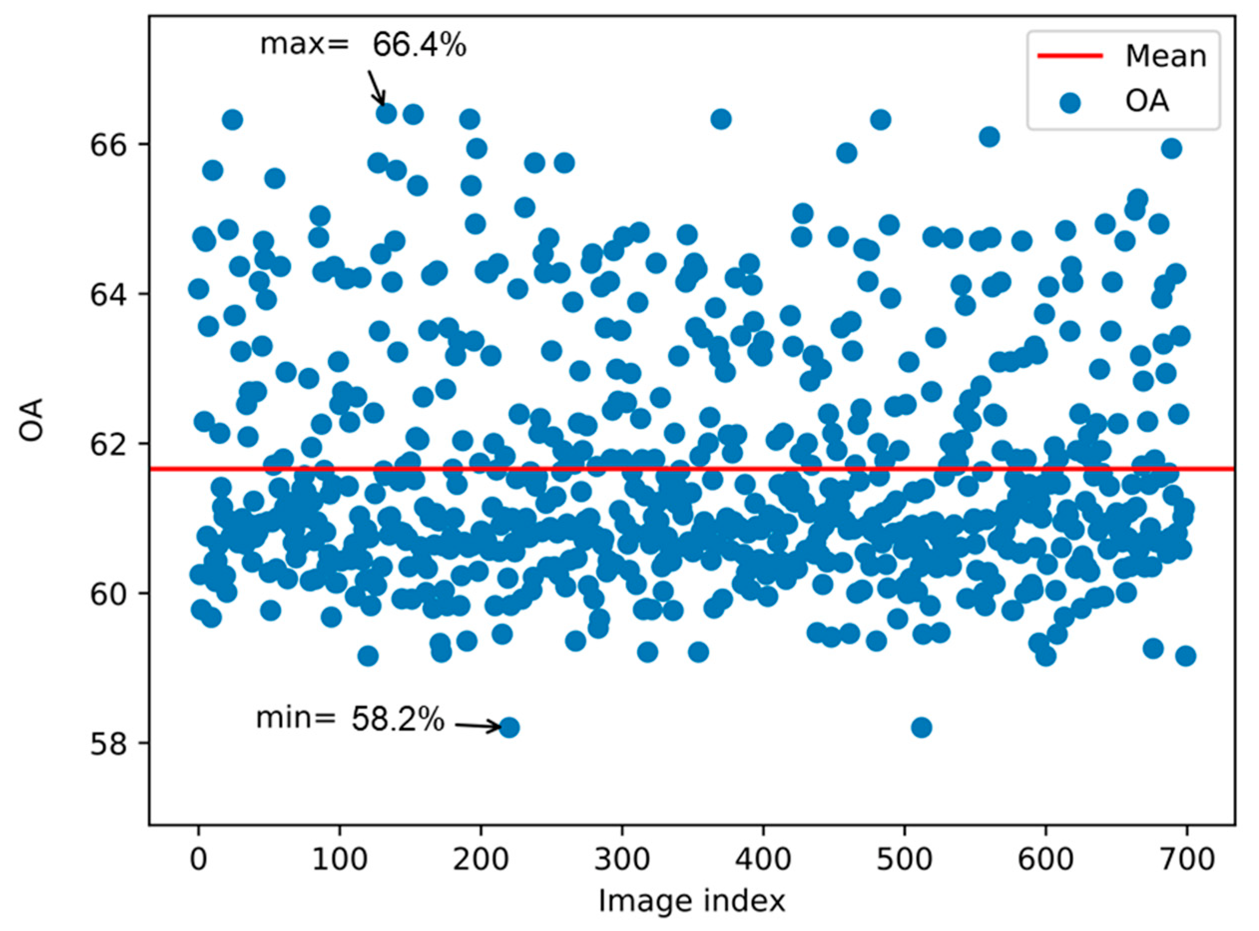
We analyzed each of the 700 obtained angles to explore the potential existence of regular patterns. Figure 3 shows the overall classification accuracy obtained for each single-angle image when 5% of the pixels were employed as the training set and 95% of the pixels were employed as the testing set in the SVM classification method. The overall accuracies (OAs) of the classification results were distributed between 58.2% and 66.4%, and the average OA of the single-angle classification results was 61.7%.
Figure 4 shows the kappa classification value of every single-angle image when 5% of the pixels were utilized as the training set and 95% were employed as the testing set in the SVM classification method. The Kappa values were distributed between 47.8% and 58.7%.
Figure 5 is a confusion matrix of the classification results derived when single-angle images were employed as the input data, with 5% of the pixels used as the training set and 95% used as the testing set in the SVM classification method. We identified only 3 land cover classes with producer’s accuracy, which indicates the probability of the ground real reference data correctly classified scores above 80% and 4 land cover classes with user’s accuracy, which indicates the ratio of the inspection points falling on the certain category correctly classified in the classification result figure scores above 80%. The producer’s accuracy scores of 4 land cover classes and the user’s accuracy scores of 2 land cover classes were below 40%. All business district pixels were classified incorrectly when only the single-angle images obtained at the same observation angle were employed. In the following experiment, an incredible classification accuracy increase was observed for this land cover class.
The use of only one observation angle may have introduced random variations that can prevent the discovery of regular trends. Therefore, we repeated the above experiment 9 more times using the 9 other angles and calculated the average values to build the same confusion matrix containing the classification results, as shown in Figure 6.
Similar to the results shown in Figure 5, certain land cover types, such as grasslands, factory district buildings, trees and asphalt roads, can be classified with high producer’s accuracies when only single-angle images are used.
However, the classification results obtained for the other land cover types were very poor, and the producer’s accuracies of certain land cover types were even below 5%. More than 7900 pixels were incorrectly classified as factory district buildings. Thus, we concluded that residential district buildings, business district buildings, and bare soils are hard to distinguish from factory district buildings when classification is performed based on only single-angle images. In the following experiment, we discovered that multiangle images are clearly superior for classifying these four land cover types.

3.2. Confusion Matrix Comparative Analysis between Single-Angle Images and Multiangle Images

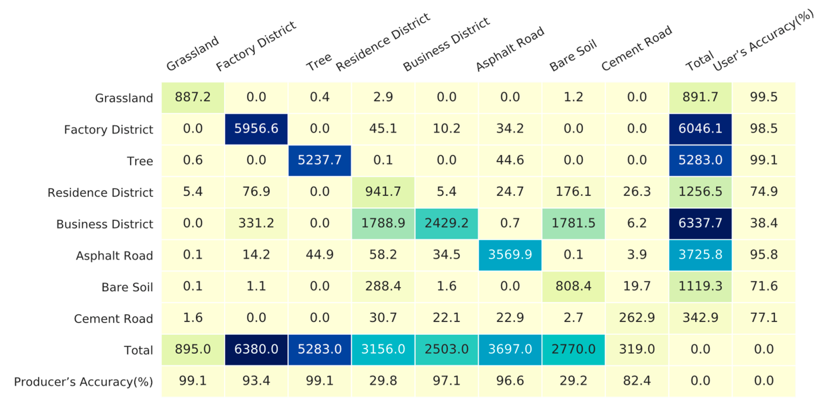
The use of images taken at multiple observation angles provides more useful classification information than single-angle images. As predicted, compared with the single-angle-image data classification results, the use of multiangle images yielded obvious improvements. We chose 32-angle images and 700-angle images for analysis. For example, Figure 7 shows the results of one classification experiment conducted using 32-angle images with 5% of the pixels utilized as the training set and the remaining 95% utilized as the testing set in the SVM classification method.
To reduce the occurrence of deviations due to the use of different angle combinations among the 32-angle images, we randomly selected 32 angles among the 700 angles, repeated the experiment 10 times and calculated the average results. Thus, the pixel counts in Figure 8 correspond to decimal values. We analyzed business district buildings. For example, the average producer’s accuracy score of business district buildings improved from 0% to 97.1%, while the corresponding user’s accuracy improved from 0% to 38.4%. The classification accuracy of every land cover type increased, except the producer’s accuracy of factory district buildings, which decreased from 97.7% to 93.4%, and the user’s accuracy of concrete roads, which decreased from 84.6% to 77.1%. However, on the whole, compared with the use of single-angle images as input data, the overall accuracy obtained when 32-angle images were utilized reflected an obvious improvement.
Figure 9 shows the classification results obtained when 700-angle images were employed, with 5% of the pixels utilized as the training set and the remaining 95% of the pixels employed as the testing set in the SVM classification method. We discovered that the accuracy of each land cover type increased, except for the producer’s accuracy scores of the business district buildings and concrete roads, as well the user’s accuracy scores of the residence district buildings, all of which decreased slightly. Similar to the comparison between the 32-angle images and the single-angle images, the use of the 700-angle images yielded an OA increase, compared with the use of the 32-angle images.
An interesting discovery made during this experiment was that for certain land cover types, such as residence district buildings, the producer’s accuracy decreased and then increased as the number of angles considered in the image data increased. This finding shows that the use of a larger number of observation angles usually introduces more information that is useful for classifying most land cover types. However, in certain situations, redundant observation information can introduce errors for certain land cover types.

3.3. Results Derived Using the SVM Classification Method

The classification percentage results derived using different training sample ratios and different observation angle numbers based on the SVM classification method are listed in Table 2. To reduce the influence of the angle selection scheme, we repeated each experiment 10 times with randomly selected angles and calculated the average percentages when constructing Table 2.
According to the training set ratios listed in Table 2, each training set was built by randomly selecting the corresponding proportion of data among all samples, while all remaining samples were utilized as the test set. The number of observation angles corresponds to the specified number of observation angles selected for the classification experiments. Theoretically, the higher the proportion of training samples was, the greater the amount of information was learned, which was helpful for obtaining more classification information and thus higher classification accuracies. Moreover, the larger the number of observation angles involved in the classification experiments and the richer the classification information contained in these data were, the higher the resulting classification accuracy was. The experimental results also show that this principle was basically consistent among the experiments conducted using different quantities of observation angle data.
The classification results derived based on the SVM method show that with the same number of observation angles, the use of an increased number of training samples produced a relatively small classification accuracy improvement, while with the same number of training samples, the use of an increased number of observation angles yielded greater improvement in the overall classification accuracy. For instance, when only two observation angles were involved in the classification experiments, the overall classification accuracy obtained when 80% of the samples were employed for training only increased from 60.6% to 67.3% compared with the 6.6% increase obtained when 1% of the samples were in the training set. When 1% of the samples were used for training with the 700-observation-angle data, the overall classification accuracy improved from 60.6% to 75.1%, reflecting an increase of 14.4%. When the commonly employed 5% ratio and 10% ratio were used to build the training sets and when 700 observation angles were compared with two observation angles, the overall classification accuracies increased by 17.6% and 18.2%, respectively, thus greatly improving the overall classification accuracy, especially for nearly indistinguishable features.
The highest classification accuracy was obtained when the maximum number of observation angles and the highest training sample proportion were utilized. This finding also conforms to the theoretical law supported by our previous assumptions.
When few observation angles were used, for example, when the number of observation angles was less than 256, and especially when the number of observation angles was less than 32, increasing the amount of considered observation angle information improved the classification accuracy of urban areas. For example, when 10% of the samples were employed as the training data, adding information from two observation angles induced a 5% improvement in the classification accuracy. Additionally, when many observation angles were available, for example, when there were more than 256 observation angles, the continual addition of more observation angles, e.g., when 10% of the samples were applied as the training data to provide information on the 256 observation angles, a classification accuracy improvement of only 0.3% was obtained. At this time, if the amount of considered observation angle information continued to increase, the classification accuracy improvement became relatively limited, that is, when few observation angles are available, increasing the amount of observation angle information can provide more useful information for classification and can greatly improve the overall classification accuracy. However, when many observation angles are already available, the addition of observation angle information can produce less useful information for classification and thus has a limited effect on improving the overall classification accuracy.

3.4. Results Derived Using the Ensemble Learning Classification Method

The classification results obtained in accordance with the use of different training sample ratios and observation angle numbers in the ensemble learning classification method are listed in Table 3.
According to the training set ratios listed in Table 3, each training set was built by randomly selecting the corresponding proportion of data among all samples, while all remaining samples were applied as the test set. The number of observation angles corresponds to the specified number of observation angles selected for the classification experiments. Similar to the trends obtained in the SVM experimental results, theoretically, the higher the proportion of training samples was, the greater the amount of helpful information for classification was learned. Thus, the higher the classification accuracy was, the larger the number of observation angles involved in the classification experiments, and the richer the classification information contained in these data were, the higher the resulting classification accuracy was. The experimental results also show that in experiments with different quantities of observation angle data, regardless of whether the SVM method or ensemble learning method was used, the findings basically conformed to the rules described above. The highest classification OA was achieved when the largest possible amount of observation angle information and the highest proportion of training samples were applied.
Similar to the conclusions drawn from the SVM classification results, when using the ensemble learning-based classification method, increasing the amount of observation angle information more effectively improved the classification accuracy compared with increasing the number of training samples. Similarly, when information from fewer than 256 observation angles was considered, the addition of more observation-angle information significantly improved the classification accuracy. When information from more than 256 observation angles was considered, the continual addition of more observation-angle information had less of a role in improving the classification accuracy.
The classification accuracy obtained using the ensemble learning-based classification method was slightly lower than that obtained using the SVM-based classification method. However, certain parameters exhibited higher classification accuracies in the ensemble learning-based results than in the SVM-based results. For example, when 2.5% of the samples were employed as the training dataset and the number of considered observation angles was greater than or equal to 4, the classification accuracy derived based on the ensemble learning method was higher than that derived based on the SVM method. This finding indicates that when classifying complex urban features using video satellite data, different classification methods may have distinct advantages and disadvantages under different parameter conditions.

4. Discussion

The experiments described in this paper show that, compared with traditional optical remote sensing satellite data, video remote sensing satellite data can be used to better distinguish complex urban features, to effectively improve the classification accuracy of complex urban features, and to classify certain subdivided urban features by category, such as various concrete roads constructed of the same materials and certain commercial, residential and factory buildings. These classifications are difficult to perform using traditional optical remote sensing satellite data. Regarding the application of video satellite data for classification tasks, the information provided by different observation angles comprises both redundant information and complementary information. The use of an increased amount of satellite observation-angle information usually yields a higher classification accuracy, especially when relatively few observation angles are available, and the average classification accuracy improves obviously as each new observation angle is considered. Regarding the video satellite data considered in this paper, when data were available for fewer than 256 observation angles, increasing the amount of observation angle information could significantly improve the classification OA. When data were available for more than 256 observation angles, if additional observation angle information was provided, the improvement in the classification OA was limited.

5. Conclusions

According to the characteristics of video satellite data, this paper reduced the data dimensions and then classified many ground features, including various urban building types, based on the following machine learning methods: SVM and ensemble learning. The results show that video satellite data are better than traditional remote sensing satellite data and contain richer information. Generally, the use of more observation angle information enables better classification accuracies and the effective classification of buildings, roads and other features in different urban areas. In this paper, the analysis results obtained with regard to the improved classification OAs from the consideration of observation angle information can serve as the basis and fundamental information for constructing the parameters of a new generation of video remote sensing satellites, which are specifically designed for urban remote sensing research in the future. Video satellite data have great potential with regard to the remote sensing classification of complex urban features. With the research foundation provided in this paper, video satellite data research involving the remote sensing of urban complex features can be effectively promoted in the future.

Author Contributions

F.Y. and T.A. conceived of and designed the experiments; J.W. performed the experiments; Y.Y. and Z.Z. analyzed the data; and F.Y. and Z.Z. wrote the paper. All authors have read and agreed to the published version of the manuscript.

Funding

Funding for this research was provided by the National Key Research and Development Program of China (grant number 2019YFC0408901), the National Key Research and Development Program of China (grant number 2018YFB2100500), and the ”Spatial monitoring of the environmental and ecological sustainable development in the Lancang-Mekong region” project (project number BF2102).

Institutional Review Board Statement

Not applicable.

Informed Consent Statement

Not applicable.

Data Availability Statement

Not applicable.

Acknowledgments

We would like to thank Chang Guang Satellite Technology Co., Ltd. for providing the remote sensing experimental data.

Conflicts of Interest

The authors declare no conflict of interest.

References

  1. Gu, Y.; Liu, H.; Wang, T.; Li, S.; Gao, G. Deep feature extraction and motion representation for satellite video scene classification. Sci. China Inf. Sci. 2020, 63, 93–107. [Google Scholar] [CrossRef] [Green Version]
  2. Hu, F.; Xia, G.S.; Hu, J.; Zhang, L. Transferring deep convolutional neural networks for the scene classification of high-resolution remote sensing imagery. Remote Sens. 2015, 7, 14680–14707. [Google Scholar] [CrossRef] [Green Version]
  3. Gu, Y.; Wang, T.; Jin, X.; Gao, G. Detection of Event of Interest for Satellite Video Understanding. IEEE Trans. Geosci. Remote Sens. 2020, 58, 7860–7871. [Google Scholar] [CrossRef]
  4. Mou, L.; Zhu, X.X. Spatiotemporal Scene Interpretation of Space Videos via Deep Neural Network and Tracklet Analysis. In Proceedings of the 2016 IEEE International Geoscience and Remote Sensing Symposium (IGARSS), Beijing, China, 11–16 July 2016; pp. 1823–1826. [Google Scholar] [CrossRef]
  5. Liu, C. Study on ground feature characteristics of multi angle remote sensing satellite images. Surv. Mapp. Tech. Equip. 2021, 23, 5. [Google Scholar]
  6. Yang, X.F.; Wang, X.M. Classification of MISR multi- angle imagery based on decision tree classifier. J. Geo-Inf. Sci. 2016, 18, 416–422. [Google Scholar] [CrossRef]
  7. Yang, X.F.; Ye, M.; Mao, D.L. Multi-angle remote sensing image classification based on artificial bee colony algorithm. Remote Sens. Land Resour. 2018, 30, 48–54. [Google Scholar]
  8. Zhang, H.; Yang, Z.; Zhang, L.; Shen, H. Super-resolution reconstruction for multi-angle remote sensing images considering resolution differences. Remote Sens. 2014, 6, 637–657. [Google Scholar] [CrossRef] [Green Version]
  9. Kong, F.; Li, X.; Wang, H.; Xie, D.; Li, X.; Bai, Y. Land cover classification based on fused data from GF-1 and MODIS NDVI time series. Remote Sens. 2016, 8, 741. [Google Scholar] [CrossRef] [Green Version]
  10. Chen, B.; Huang, B.; Xu, B. Multi-source remotely sensed data fusion for improving land cover classification. ISPRS J. Photogramm. Remote Sens. 2017, 124, 27–39. [Google Scholar] [CrossRef]
  11. Chen, C.; Knyazikhin, Y.; Park, T.; Yan, K.; Lyapustin, A.; Wang, Y.; Yang, B.; Myneni, R.B. Prototyping of lai and fpar retrievals from modis multi-angle implementation of atmospheric correction (maiac) data. Remote Sens. 2017, 9, 370. [Google Scholar] [CrossRef] [Green Version]
  12. Hall, F.G.; Hilker, T.; Coops, N.C.; Lyapustin, A.; Huemmrich, K.F.; Middleton, E.; Margolis, H.; Drolet, G.; Black, T.A. Multi-angle remote sensing of forest light use efficiency by observing PRI variation with canopy shadow fraction. Remote Sens. Environ. 2018, 112, 3201–3211. [Google Scholar] [CrossRef] [Green Version]
  13. Xu, Y.; Ren, C.; Cai, M.; Edward, N.Y.Y.; Wu, T. Classification of local climate zones using ASTER and Landsat data for high-density cities. IEEE J. Sel. Top. Appl. Earth Obs. Remote Sens. 2017, 10, 3397–3405. [Google Scholar] [CrossRef]
  14. Shao, Z.; Zhou, Z.; Huang, X.; Zhang, Y. MRENet: Simultaneous Extraction of Road Surface and Road Centerline in Complex Urban Scenes from Very High-Resolution Images. Remote Sens. 2021, 13, 239. [Google Scholar] [CrossRef]
  15. Xu, K.; Jiang, Y.; Zhang, G.; Zhang, Q.; Wang, X. Geometric potential assessment for ZY3-02 triple linear array imagery. Remote Sens. 2017, 9, 658. [Google Scholar] [CrossRef] [Green Version]
  16. Zhang, G.; Li, L.T.; Jiang, Y.H.; Shi, X.T. On-orbit relative radiometric calibration of optical video satellites without uniform calibration sites. Int. J. Remote Sens. 2019, 40, 5454–5474. [Google Scholar] [CrossRef]
  17. Wu, J.; Wang, T.; Yan, J.; Zhang, G.; Jiang, X.; Wang, Y.; Bai, Q.; Yuan, C. Satellite video point-target tracking based on Hu correlation filter. Chin. Space Sci. Technol. 2019, 39, 55–63. [Google Scholar]
  18. Li, H.; Chen, L.; Li, F.; Huang, M. Ship detection and tracking method for satellite video based on multiscale saliency and surrounding contrast analysis. J. Appl. Remote Sens. 2019, 13, 026511. [Google Scholar] [CrossRef]
  19. Joe, J.F. Enhanced Sensitivity of Motion Detection in Satellite Videos Using Instant Learning Algorithms. In Proceedings of the IET Chennai 3rd International Conference on Sustainable Energy and Intelligent Systems (SEISCON 2012), Tiruchengode, India, 27–29 December 2012; pp. 424–429. [Google Scholar]
  20. Shao, Z.; Cai, J.; Wang, Z. Smart monitoring cameras driven intelligent processing to big surveillance video data. IEEE Trans. Big Data 2017, 4, 105–116. [Google Scholar] [CrossRef]
Figure 1. Experimental image and ground-truth data (a) and the corresponding image obtained from the satellite video remote sensing data (b). The reference satellite-derived remote sensing data from Google Earth (c) and the labeled ground truth data.
Remotesensing 14 02324 g001
Figure 2. Main flow chart of the experimental methods.
Remotesensing 14 02324 g002
Figure 3. Classification OA when obtained single-angle images were utilized as the input data. The red line represents the average OA of every single-angle classification OA result.
Remotesensing 14 02324 g003
Figure 4. Kappa values of the classification results derived when a single-angle image was used as the input data. The red line represents the average of every single-angle kappa value of the classification results.
Remotesensing 14 02324 g004
Figure 5. Confusion matrix of classification results when only single-angle images according to one angle served as the input data.
Remotesensing 14 02324 g005
Figure 6. Confusion matrix of the classification results derived when single-angle images were employed as the input data (average values obtained with single-angle images corresponding to 10 angles).
Remotesensing 14 02324 g006
Figure 7. Confusion matrix of the classification results obtained when one set of 32-angle images was employed as the input data.
Remotesensing 14 02324 g007
Figure 8. Confusion matrix of the classification results obtained when 32-angle images were selected as input data (representing the average values obtained in 10 iterations).
Remotesensing 14 02324 g008
Figure 9. Confusion matrix of the classification results derived when 700-angle images were selected as the input data.
Remotesensing 14 02324 g009
Table 1. Ground truth land cover classes and the corresponding numbers of samples.
No.Class NameNumber of Samples
1Grasslands924
2Trees6715
3Bare soils5561
4Building (factory district)3322
5Building (residential district)2634
6Building (business district)3891
7Asphalt roads2915
8Concrete roads335
Total\26,315
Table 2. Classification OAs derived using the SVM method.
Training Set Radio1%2.5%5%10%20%40%80%
Number of Angles
156.960.061.763.665.164.266.2
260.661.063.464.565.664.967.3
462.463.169.169.569.569.772.8
865.769.772.173.075.976.577.0
1669.370.873.774.877.277.878.6
3270.373.176.878.179.480.280.9
6470.774.578.579.981.082.083.1
12871.376.979.781.382.683.784.9
25671.577.080.582.183.784.885.9
51271.677.780.782.484.285.485.5
70075.178.081.082.785.185.688.0
Table 3. Classification OAs derived using the ensemble learning method.
Training Set Ratio1%2.5%5%10%20%40%80%
Number of Angles
151.552.754.554.555.656.260.4
255.056.456.656.657.057.962.9
461.864.263.864.564.166.667.7
864.666.566.966.867.068.969.3
1665.970.372.471.872.472.373.5
3267.373.174.374.775.976.076.4
6468.474.676.677.477.978.078.0
12868.776.978.079.179.780.080. 8
25668.579.080.080.280.681.081.1
51268.579.680.781.181.682.282.4
70072.081.080.881.481.982.783.0
Publisher’s Note: MDPI stays neutral with regard to jurisdictional claims in published maps and institutional affiliations.