Article

Using Satellite NDVI Time-Series to Monitor Grazing Effects on Vegetation Productivity and Phenology in Heterogeneous Mediterranean Forests

1
Computational Biology and Population Genomics Group, Centre for Ecology, Evolution and Environmental Changes, Departamento de Biologia Animal, Faculdade de Ciências, Universidade de Lisboa, Campo Grande, 1749-016 Lisboa, Portugal
2
MARETEC/LARSyS, Instituto Superior Técnico, Universidade de Lisboa, Av. Rovisco Pais 1, 1049-001 Lisboa, Portugal
3
Terraprima—Serviços Ambientais, Sociedade Unipessoal, Lda, 2135-199 Samora Correia, Portugal
4
Terraprima—Sociedade Agrícola, Lda, Apartado 8, Quinta da França—Teixoso, 6250-111 Caria BMT, Portugal
*
Author to whom correspondence should be addressed.
Remote Sens. 2022, 14(10), 2322; https://doi.org/10.3390/rs14102322
Submission received: 12 April 2022 / Revised: 7 May 2022 / Accepted: 8 May 2022 / Published: 11 May 2022
(This article belongs to the Section Environmental Remote Sensing)

Abstract

:
The reintroduction of livestock grazing to regulate biomass load is being tested for large-scale restoration in Mediterranean landscapes affected by rural abandonment. Concurrently, there is a need to develop cost-effective methods to monitor such interventions. Here, we investigate if satellite data can be used to monitor the response of vegetation phenology and productivity to grazing disturbance in a heterogenous forest mosaic with herbaceous, shrub, and tree cover. We identify which vegetation seasonal metrics respond most to grazing disturbances and are relevant to monitoring efforts. The study follows a BACI (Before-After-Control-Impact) design applied to a grazing intervention in a Pyrenean oak forest (Quercus pyrenaica) in central Portugal. Using NDVI time-series from Sentinel-2 imagery for the period between June 2016 and June 2021, we observed that each type of vegetation exhibited a distinct phenology curve. Herbaceous vegetation was the most responsive to moderate grazing disturbances with respect to changes in phenology and productivity metrics, namely an anticipation of seasonal events. Results for shrubs and trees suggest a decline in peak productivity in grazed areas but no changes in phenology patterns. The techniques demonstrated in this study are relevant to a broad range of use cases in the large-scale monitoring of fine-grained heterogeneous landscapes.

1. Introduction

Large herbivores play a critical role in ecosystem functioning; they contribute to the regulation of vegetation structure and composition, maintenance of habitat diversity, seed dispersal, and nutrient recycling [1,2,3]. Their effects on ecosystems are associated both with biomass consumption (i.e., herbivory) and with mechanical disturbances, such as trampling and wallowing. In some world regions, and particularly in the Mediterranean basin, the populations of wild herbivores have historically been depleted, and their ecological role has been largely replaced by livestock in extensive grazing regimes [4,5]. More recently, during the last half-century, socioeconomic changes have been driving the abandonment of marginal agricultural land, including grazing areas [5,6,7]. Abandoned areas have experienced two main land-use-change trajectories: afforestation or natural revegetation driven by secondary succession. In both cases, active biomass management may be neglected, or even absent, due to the low benefit–cost ratio [8,9]. This results in unregulated biomass growth with shrub and tree encroachment, which leads to an increased risk of wildfire and impairs the sustainability of these landscapes.
For these reasons, the reintroduction of grazing by large domestic herbivores is being regarded as a nature-based solution to counteract and address the risks of unregulated biomass growth in marginal land [10,11,12]. This method has the advantage of being applicable on large scales, such as in landscape restoration, and of being potentially cost-effective when compared to other management options [13,14].
If adequately managed, the reintroduction of livestock grazing is expected to generate moderate levels of ecological disturbance and contribute to the restoration or maintenance of habitat and species diversity, regulate biomass growth and vegetation structure, and promote nutrient cycling and seed dispersal [3,15,16]. On the other hand, grazing regimes need to be carefully monitored and adjusted to avoid the risk of overgrazing and other associated impacts, such as soil degradation, low tree regeneration, a decline in vegetation productivity and in species diversity, and lower resilience to environmental pressures [17,18,19].
Hence, these approaches require monitoring techniques that can be applied to large spatial scales, without compromising the spatial and temporal resolutions, to ensure an effective evaluation and monitoring of the results. The increasing spatial, temporal, and spectral resolutions of Earth-observation satellites pushes forward the use of remote sensing as a means of generating large-scale understandings, at low cost, of ecosystem conditions and environmental changes [20,21].
In the case of landscape vegetation monitoring, vegetation seasonal metrics, namely phenology and productivity metrics, are a good example of information that can be retrieved from remotely sensed imagery. Phenology can be defined as the timing of the development of photosynthetically active leaf foliage, and phenological parameters are the metrics used to describe the stage of the vegetation seasonal growth curve or phenology curve [22]. Therefore, phenology, which is monitored using phenology metrics, is intimately related to the variation in photosynthetic activity and vegetation growth, which is monitored using productivity metrics. Phenology curves, which show the temporal dynamics (i.e., changes in the value) of photosynthetic activity, are produced from time-series of primary productivity data, which, for their part, can be estimated using remotely sensed vegetation indexes based on the spectral reflective behavior of the vegetation. In particular, the level of vegetation greenness can be assessed from the comparison of reflectance in the near-infrared and red wavelengths, where the greener the vegetation, the more it will reflect light in the near-infrared and absorb in the red wavelength [23].
Remotely sensed phenology and productivity metrics are extracted from the phenology curves (Table 1, Appendix A, Figure A1) and can be used to infer vegetation seasonal dynamics and responses to environmental changes. This includes parameters associated with the timing of seasonal events, such as the start and end times of the growing season or season length, and the parameters associated with the values of productivity, such as the maximum or base productivity, the seasonal amplitude, or the small and large seasonal integrals [24].
In this work, we investigate if remotely sensed satellite data can be used to detect and monitor changes in phenology and productivity patterns in a deciduous forest mosaic, composed of different types of vegetation cover, namely herbs, shrubs, and trees, and characterized by high heterogeneity and fine spatial grain. We aim to identify which vegetation seasonal metrics respond to grazing disturbance and can be used to monitor and assess the effects of grazing interventions in this type of landscape.
More specifically, and when compared with areas under natural succession without grazing, the areas with moderate grazing are expected to show higher productivity of the herbaceous layer due to the reduction of self-shading by the standing senescent biomass, which prevents seed germination and plant growth [26]. Grazing was also shown to be associated with a compensation mechanism in herbaceous vegetation, where plants increase their growth rate to account for the suffered herbivory damages [26]. On the other hand, a declining trend in herbaceous productivity and in the annual minimum NDVI value could suggest an increase in bare ground due to overgrazing [27]. The effect of herbivory and trampling is also expected to cause a decline in shrub productivity due to the loss of photosynthetic structures [28]. Finally, the impacts of moderate livestock grazing are expected to be less severe on trees (especially on adult trees) than on other vegetation types. Hence, we do not anticipate grazing-driven changes. However, if present, declines in canopy greenness may indicate direct or indirect negative impacts on tree condition (e.g., mechanical damage to bark and branches, indirect effects from changes in soils features due to overgrazing) and the need to adjust the grazing regime.

2. Materials and Methods

2.1. Study Area

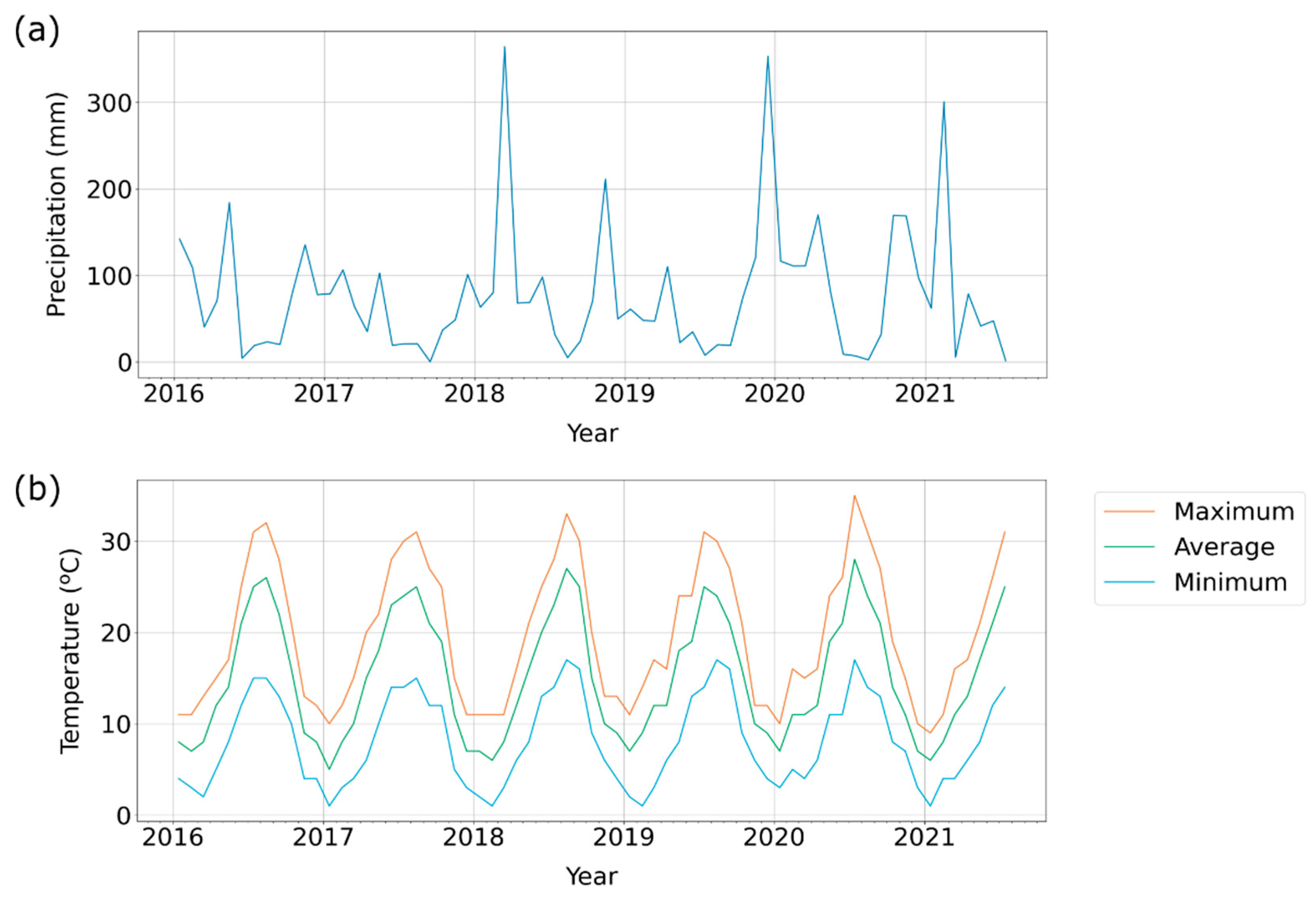
This study uses data from a Pyrenean oak forest (Quercus pyrenaica, Habitats Directive 9230) of about 200 ha, located in Quinta da França (Covilhã, Portugal, Figure 1a,b). This is a farm with multiple lands uses, including production and conservation forest, cereal crops, meadows, and pastures for livestock production (https://www.terraprima.pt/en/area-de-actividade/4, accessed on 6 May 2022). The climate is generally warm, with an average annual temperature of 12.6 °C and precipitation of 1012 mm (https://en.climate-data.org/europe/portugal/covilha/covilha-6944/, accessed on 14 September 2021). During the study period, the temperature ranged from 1 °C in January 2017 to 35 °C in July 2020. As for precipitation, March 2018 was the wettest month with 364.23 mm of accumulated rainfall, while September 2017 was the driest with 0.1 mm (Appendix A, Figure A2).
Regarding vegetation cover, the forest area is composed of tree-covered patches of varied sizes and densities, interspersed with shrubs and herbaceous vegetation (Figure 1c). The dominant species, Quercus pyrenaica, is a deciduous tree native to the Iberian Peninsula, where it has most (95%) of its distribution. As for the shrub layer, it is largely dominated by broom species (Cytisus multiflorus and C. scoparius). Hawthorn (Crataegus monogyna), blackberry (Rubus ulmifolius), and grey willow (Salix atrocinerea) are also present.
The forest study area has been under natural regeneration since two large fires in 1983 and 1995 and is now managed mostly for carbon storage and sequestration and conservation purposes. Periodic shrub clearing with mechanized tools has been used to prevent shrub encroachment and the risk of wildfires, with the last general intervention dating to 2010 (specific interventions, such as road maintenance, are more frequent and those areas were excluded from the analyses). More recently, in 2018, as part of the SILVPAST project (https://www.terraprima.pt/en/projecto/23, accessed on 6 May 2022), the oak forest was divided into two large sectors by a fence installed halfway (Figure 1b,c). A herd of approximately 60 cows was given access to the south sector in June 2018, while the north sector remained closed to grazing. Since then, the herd has had permanent access to the forest while also grazing on rainfed and irrigated pastures in the vicinity (total grazing area, including forest and pastures, of about 180 ha). This management intervention aims to test the use of cattle grazing as a nature-based solution to regulate vegetation structure and biomass loads. Wild herbivores, such as roe deer, are present in both sectors but in low abundance.

2.2. Study Design

The study follows a BACI (Before-After-Control-Impact) design, that is, its time interval spans from two years before to three years after the start of the grazing intervention and uses data from both forest sectors (Figure 1b). The north sector is used as a control area, and the south sector is used as an impact/test area. This type of study design is recommended for its robustness, because, when applied to areas sharing equivalent environmental conditions and exposed to the same natural and other background drivers of change, it allows for the singling out of the effect of the management intervention from background changes (e.g., interannual climate variability), thus reducing the potential bias from confounding variables [29,30].
Here, we use an NDVI time-series from Sentinel-2 imagery to analyze vegetation phenology from June 2016 to June 2021 and assess its response to cattle grazing. Vegetation phenology is examined separately for the three main types of vegetation cover in the oak forest mosaic: herbs, shrubs, and trees. A landcover map of 2020 with a pixel size of 20 cm (Figure 1c), produced from drone imagery and available from the farm managers, was upscaled using the 10 m × 10 m pixel grid of Sentinel-2. The dominant vegetation cover in each grid cell was defined using the following rules: cells with tree cover >80% were classified as tree areas; cells with tree cover <30%, herbaceous cover <30%, and shrub cover >50% were classified as shrub areas; and cells with herbaceous cover >70% as herbaceous areas; remaining cells not meeting any of these criteria were excluded from the analysis. Note, however, that the percentage of landcover only relates to the top vegetation layer visible from above (i.e., aerial image), so it does not reflect the vertical stratification at each point. We also excluded from the analysis those areas that had been subjected, since 2016, to any type of vegetation management, such as road maintenance or vegetation clearing for fence installation. Moreover, in the south sector, we only kept areas that were effectively used by cattle to ensure representativeness in the analyses. For that purpose, cattle movement data, collected with three GPS collars between 2018 and 2020, were analyzed on ArcGIS (version 10.7.1). We applied a conservative approach by only selecting GPS locations that were within a range of 50 m from each other and discarding movement outliers. Following outlier removal, frequent grazing areas (Figure 1b) were defined as the areas within a 50 m buffer of the selected location points. The upscaled landcover layer was then intersected with the limits of the two forest sectors (without excluded areas) and the NDVI layers, to classify and select all the eligible 10 m × 10 m pixels of the Sentinel-2 grid into six non-overlapping landcover groups, considering landcover in 2020: in the north sector, trees (3763 pixels), shrubs (554 pixels), and herbs (625 pixels); in the south sector, trees (1947 pixels), shrubs (118 pixels), and herbs (603 pixels). While these groups pertain to landcover in 2020, we expect the dominant landcover in each grid cell (10 m × 10 m) to have remained stable during the study period, with changes mostly occurring on a finer scale, being more gradual and nuanced, and related to changes in cover density and stratification (i.e., horizontal and vertical structures) and in ecosystem functioning, including phenology and productivity seasonal dynamics.

2.3. Satellite Data

Sentinel-2 Multispectral Instrument (MSI) orthorectified images (Level-1C) were acquired from January 2016 until June 2021. These images were automatically downloaded through Copernicus API HUB or manually downloaded from Copernicus Open Access Hub (https://scihub.copernicus.eu/, last accessed on 19 October 2021). Complete images (700 Mb) for the region’s 100 km tile (29TPE tile) that were free of clouds (≤5% clouds) were automatically selected and downloaded. For missing dates, due to the cloud-cover threshold (>5% clouds), a visual and geographic cloud-cover assessment was completed for the study area in the Sentinel Hub Playground (https://apps.sentinel-hub.com/sentinel-playground/, last accessed on 19 October 2021), and the images free of clouds were selected for download. The resulting time-series included all images of the Sentinel-2 tiles containing the study area for 5 years and 4 months, resulting in a final set of 121 images (1–4 per month).
The Normalized Difference Vegetation Index was calculated for the extent of the study area for all the available dates using Sentinel-2′s B4 (red) and B8 (near-infrared) bands [31]. The NDVI is one of the most widely used metrics in satellite vegetation monitoring [23,32]. It can be obtained by calculating the normalized difference between the near-infrared and red spectral bands (NDVI = (NIR − red)/(NIR + red)) and is positively correlated with the biophysical properties of vegetation cover and biomass [33]. Due to its correlation with plant biomass, several phenology and productivity metrics can be derived from this index. For that reason, it has been applied in a diverse range of phenology studies [34,35,36]. Moreover, due to its large-scale applicability and cost-efficiency, the NDVI has been and continues to be considered one of the most important tools in environmental research [23].

2.4. Data Analysis

Seasonal metrics were retrieved from the NDVI time-series using TIMESAT (version 3.3), a software package for time-series processing and the assessment of vegetation dynamics [24]. Due to the fact that the collected time-series had temporal gaps due to data unavailability, a Python script was used to bin the data into regular monthly time intervals as required by TIMESAT. Specifically, we selected one image per month based on the following criteria: preference was given to mid-month images (date close to the middle of the month); otherwise, preference was given to the image whose distance was closer to 30 days from the previous image/previous month. The goal of this approach was to build a monthly dataset that was as regularly timed as possible considering image availability constraints. The final dataset consisted of 60 monthly images, 1 per month during the 5-year interval between June 2016 and June 2021. The selected TIFF images were then converted to a binary format (.bin) using the GDAL library and imported to TIMESAT to perform the analysis.
An adaptive Savitzky–Golay filter was fitted to the data to reduce the noise in the time-series. A window size of four time-steps was selected for this filter, along with an adaption strength range of 2–3. The curves were fitted using TIMESAT’s TSM_GUI tool, and the default parameters values were applied to the time-series of individual pixels representative of the different landcover types. The values for the fitting parameters were accepted after verifying that fitted curves aligned with the expected seasonal parameters for the dominant type of vegetation.
The phenology and productivity metrics delivered by TIMESAT for each individual pixel were extracted from the corresponding Savitzky–Golay fitted curve. The median values were then calculated per pixel-group for group analyses of the vegetation metrics (Table 2). Moreover, for the visualization of phenological patterns, the NDVI values were imported directly from the 121 available satellite images, using Python’s GDAL library (version 3.3.2). A Savitzky–Golay filter was applied to the NDVI values on each pixel, using parameters similar to those on TIMESAT. Then, the median absolute deviation (MAD) and the median of the adjusted values were calculated for each of the six pixel-groups and plotted using Python’s Matplotlib library (version 3.4.2) (Figure 2).
Considering the Savitzky–Golay adjusted time-series, the default settings of TIMESAT were used to define the start of a growing season, that is, the time for which the left edge of the NDVI curve has increased to 20% of its maximum value. Similarly, the season is considered to end when the NDVI value drops to 20% of the maximum value. While the timing of each season varies between vegetation types and according to their growth dynamics, we can generally identify four growing seasons during the period of this study, the first two seasons (season 1 and 2) encompassed by the time-interval that starts between late 2016/early 2017 and ends between late 2018/early 2019 and the last two seasons (season 3 and season 4) encompassed by the time-interval that starts between late 2018/early 2019 and ends between late 2020/early 2021 (Figure 2). We considered these two intervals of time when assessing the impact of cattle grazing. The first interval corresponds to the first and second growing seasons, while the second interval corresponds to the third and fourth seasons, all identified using TIMESAT. Although the cattle were introduced in June 2018, the chosen time intervals are defined based on the assumption that the effect of cattle on vegetation dynamics would not be immediate and would therefore only be noticeable in the next growing seasons (i.e., seasons 3 and 4).
After dividing the time-series into two time intervals, the changes in vegetation seasonal metrics were assessed in two steps. First, by comparing phenology and productivity metrics between the two time intervals (seasons 1–2 against seasons 3–4) using paired samples of the pixels in each of the six groups (i.e., a pair of values for each single pixel, each value corresponding to a time interval). In this approach, the average value for the two growing seasons in each interval was used. This approach delivers a first assessment of changes in vegetation seasonal metrics, including the magnitude and direction of change, per vegetation type in each sector, regardless of the underlying drivers, namely climatic variability and presence or absence of grazing. Second, the magnitude and direction of the observed changes are compared between the two sectors (i.e., test if the differences are different). The aim of this analysis is to control for the natural interannual variability in vegetation dynamics and detect divergent patterns of change between the two sectors, which would be associated with the distinct trajectories in land use, that is, no intervention in the north sector versus cattle grazing in the south sector. We opted for this approach instead of a direct comparison of the sectors, because, despite being very similar, there are still differences between the two due to the natural spatial heterogeneity.
We used the paired Wilcoxon Signed-Rank tests when comparing the two time periods for each sector (step 1), and Mann–Whitney U tests when comparing the differences between sectors (step 2), as most of the metrics datasets did not meet the assumption of normality. In addition, statistical testing was complemented by visual inspection of the boxplots.
In both steps, statistically significant results were further analyzed by means of effect sizes using the Cliff’s delta value. This was necessary because sample sizes were very large (118 to 3763 pixels per group), and, therefore, the statistical significance may not reflect the practical significance [37]. The effect size informs on the magnitude of the difference between the groups and is frequently used to evaluate the extent of the effect of any type of treatment between two study groups [38].
Cliff’s delta, in particular, estimates the probability that a randomly selected observation from one sample group is larger than a randomly selected observation from another sample group, minus the reverse probability [39]. It is estimated as,
d = i , j [ x i > x j ] [ x j > x i ] m n ,
where xi are values within one group (test group), xj are values within another group (control group), and m and n are the respective sizes of the sampled groups. The Iverson bracket [∙] equals to 1 if the condition inside the square brackets is satisfied and 0 otherwise.
As such, this statistic ranges from 1 when all values in the test group are higher than the values in the control group, to −1 when the reverse is true. A Cliff’s delta of 0 (zero) means that the samples’ distributions completely overlap. Due to its non-parametric nature, Cliff’s delta reduces the impact of extreme values or of the distribution shape and is therefore suitable when data is not normally distributed or presents many outliers. For interpretation of results, we considered commonly used thresholds for this metric, with |d| < 0.147 being considered as ‘negligible’, 0.147 < |d| < 0.330 as ‘small’, 0.330 < |d| < 0.473 as ‘medium’, and |d| > 0.473 as ‘large’ [40].
Considering the description above, in the first step of the data analysis, the xi values correspond to the second time interval, being the averaged values (from seasons 3 and 4) of the phenology or productivity metrics for a given pixel, while the xj values represent the same for the first time interval (seasons 1 and 2). When dealing with productivity metrics, a positive signal of the delta value is associated with an increase in measured NDVI, and a negative value with a decrease. Regarding phenology metrics, a positive value would be associated with a delay of the date (i.e., later in time), while a negative value would be associated with an anticipation.
For the second step of the analysis, the absolute values of the differences between the two time intervals (from step 1) were used to compare the magnitude of change between sectors. Hence, xi represents the absolute values of the differences observed in the south sector for a given phenology or productivity metric in a given pixel, while xj represents the same on the north sector. In this case, delta values close to 1 would indicate that a higher degree or magnitude of change in the south sector, when compared with the north sector, while values close to −1 would indicate the reverse. In addition to the magnitude of change (assessed from the absolute values), the direction of the change (i.e., positive values indicating an increase or delay in the metrics and negative values indicating a decrease or anticipation) was assessed from the inspection of the boxplots.

3. Results

3.1. Phenology Patterns of Vegetation Types

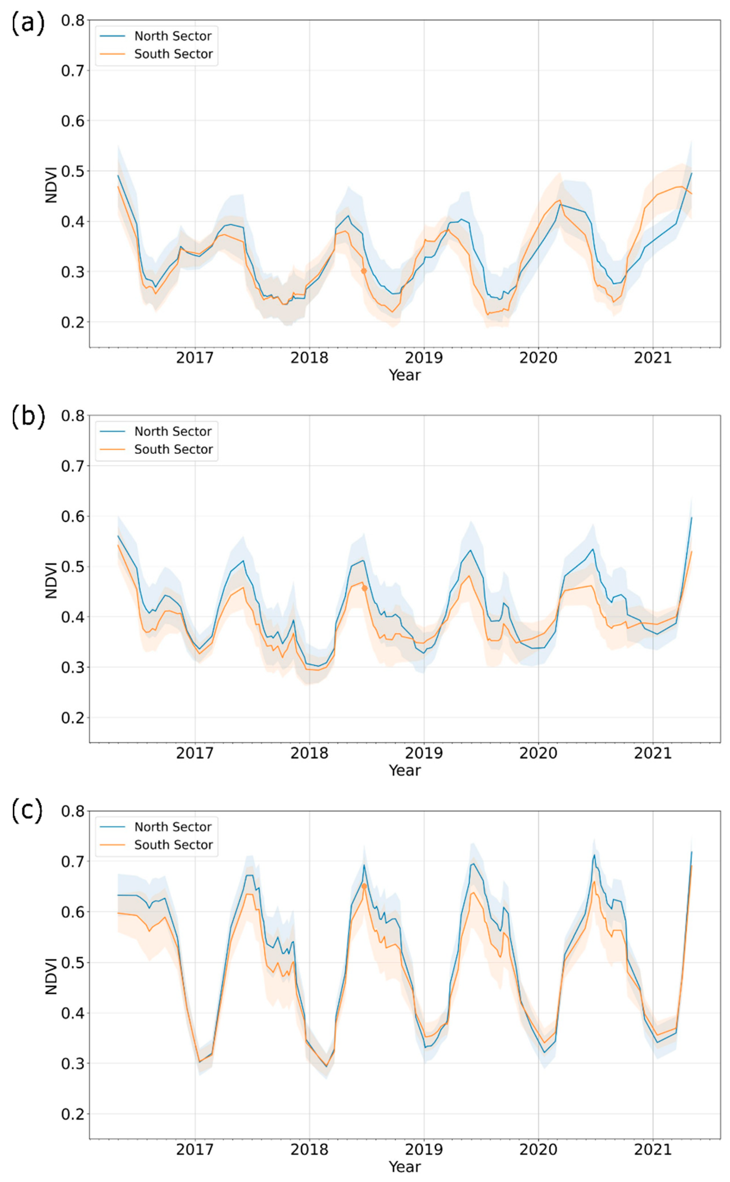
The three main types of vegetation assessed here are characterized by distinct phenological patterns (Figure 2, Table 2). The herbaceous vegetation has its growing season from autumn to summer, with a productivity peak around March and a senescent period in the summer. Shrubs start their growing season later than herbs, i.e., during the winter, reaching their maximum productivity in mid-spring, around May, after which they enter a descending phase until reaching a base value in the autumn. Finally, tree-dominated pixels displayed the most regular seasonal patterns, with growing seasons always starting at the end of the winter (early March) and coming to an end in the autumn (November), with peak productivity registered by the month of June. Both trees and shrubs show a second, smaller, peak of productivity in the autumn, around the month of November. This pattern could be related to the first events of precipitation in the autumn, which could restore shrub and tree productivity after the dry season, and it is also likely to be related to the start of the growing season of the herbs, also triggered by precipitation, in the understory of shrubs and trees. Hence, the NDVI of areas dominated by shrubs or trees (i.e., covering the top vegetation layers) also includes the signal of the herbs in the bottom layer, especially during shrubs’ and trees’ low productivity seasons, when their cover is at minimum levels or even absent (as in the case of deciduous trees).
From a temporal perspective, the phenology curves of the two sectors in the first two growing seasons seemed to be fairly aligned for all vegetation types but start to diverge after the introduction of cattle grazing in June 2018 in the south sector, especially in what regards herbaceous and shrub vegetation (Figure 2). In particular, the phenology curve of herbaceous vegetation in the south sector (Figure 2a) shows higher productivity in the initial stages of the growing season, an increase of the maximum productivity, and an earlier end time. Regarding shrubs (Figure 2b), the main changes seem to be a decrease in maximum NDVI in season 4, in the south sector, but also an increase of the base value, which may be an artifact of the presence of a more productive herbaceous layer under the shrub canopy at that time of the year. Finally, in the areas with tree cover, the phenology curve does not seem to be significantly disrupted by cattle grazing, continuing to be aligned with the curve from the north sector (Figure 2c). The most striking difference is an increase in the base NDVI value. As discussed above, this change may be associated with a stronger signal from the herbaceous layer in the understory, especially because oak trees are leafless at that time of the year.

3.2. Changes in Phenology Metrics

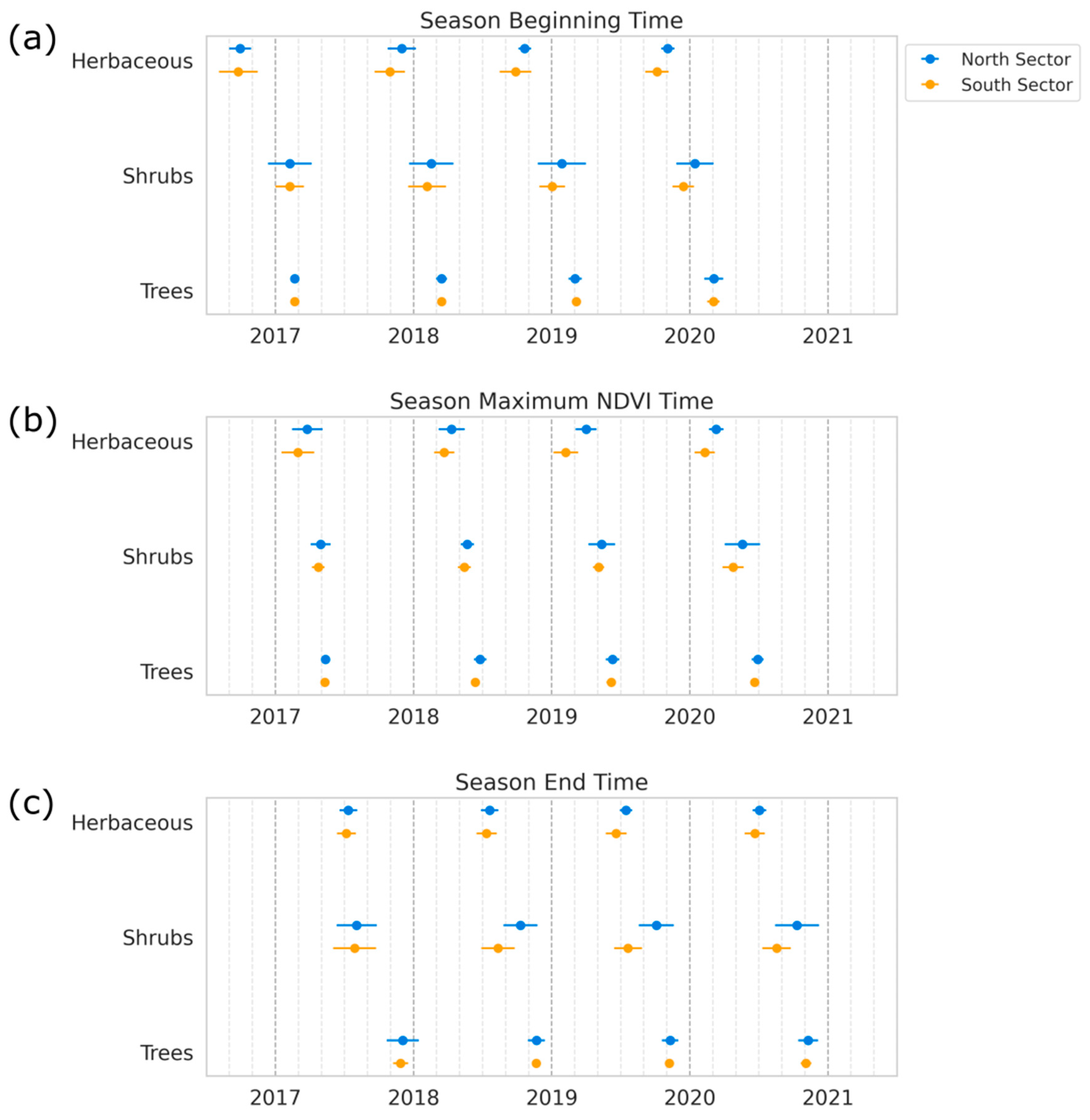
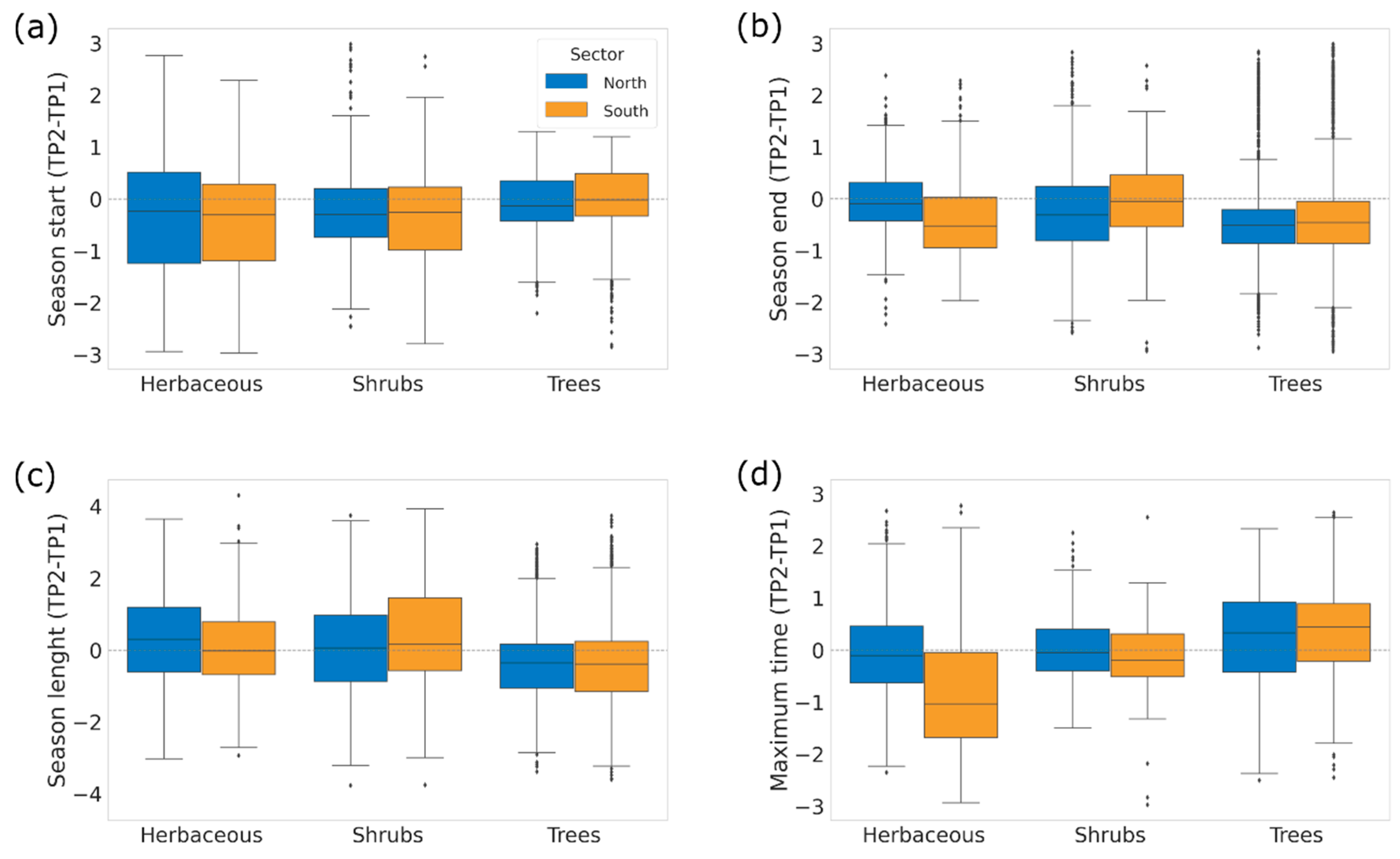
Shrub- and tree-dominated areas showed similar patterns of change between the two study periods (i.e., seasons 1–2 vs. season 3–4) in both study sectors. In the case of shrubs, the growing season started earlier in the second time period, but the end of the season did not change, which resulted in an increase in the season length (Table 3 and Table 4, Appendix A, Figure A4). Because these changes were equivalent in both study sectors (Table 5, Figure 3), they are probably driven by the same factors, in particular, by natural climatic variability. Regarding trees, the observed phenological changes included the anticipation of the end of the growing season, which consequently reduced the season length, and a delay in the timing of the peak productivity (Table 3 and Table 4, Appendix A, Figure A3). While changes were equivalent in both sectors (Table 5, Figure 3), and therefore probably driven by the same factors, the effect sizes were smaller in the south sector in relation to what constitutes the end of the season and its length. This could be due to a more vigorous signal of the herb layer in the south sector (see next paragraph and section), which starts its growing season at about the same time as the trees’ growing season ends, hence, probably masking and offsetting the decline of the trees’ signal at this time of the year.
Finally, both sectors experienced an anticipation of the end of the growing season for herbs and of their time of peak productivity (Table 3 and Table 4, Appendix A, Figure A3). However, the large values of the effect sizes indicate that this pattern was more prevalent in the south sector, while the effect sizes in the north were relatively small. This result is further confirmed by the comparison of changes between sectors, with larger changes observed in the south sector (Table 5, Figure 3), that is, the anticipation of the timing of the peak productivity and of the end of the growing season.

3.3. Changes in Productivity Metrics

Results for productivity metrics also reveal similar trajectories of change in both sectors but suggest stronger effects for all vegetation types in the south sector, some of which were driven, directly or indirectly, by grazing.
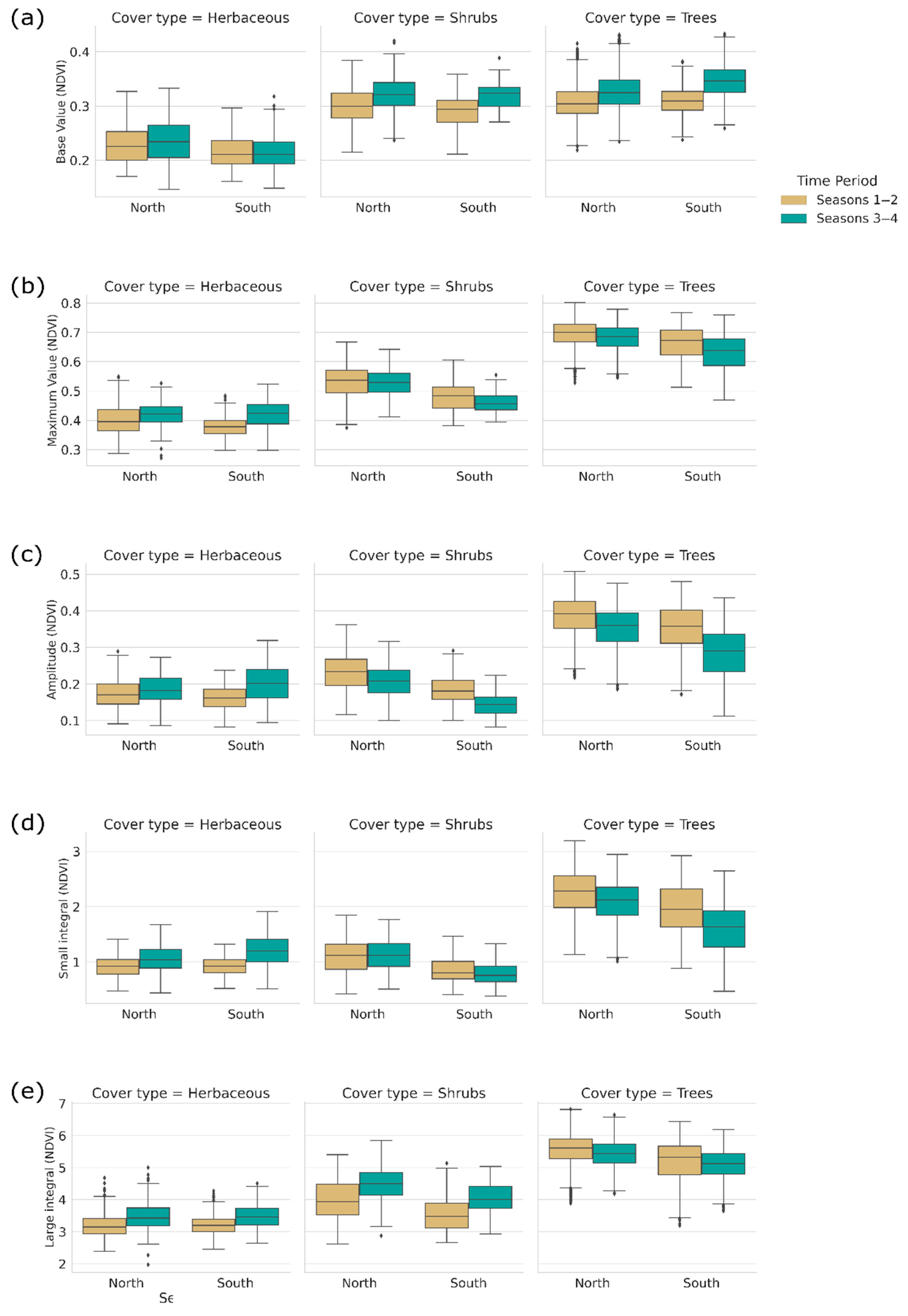
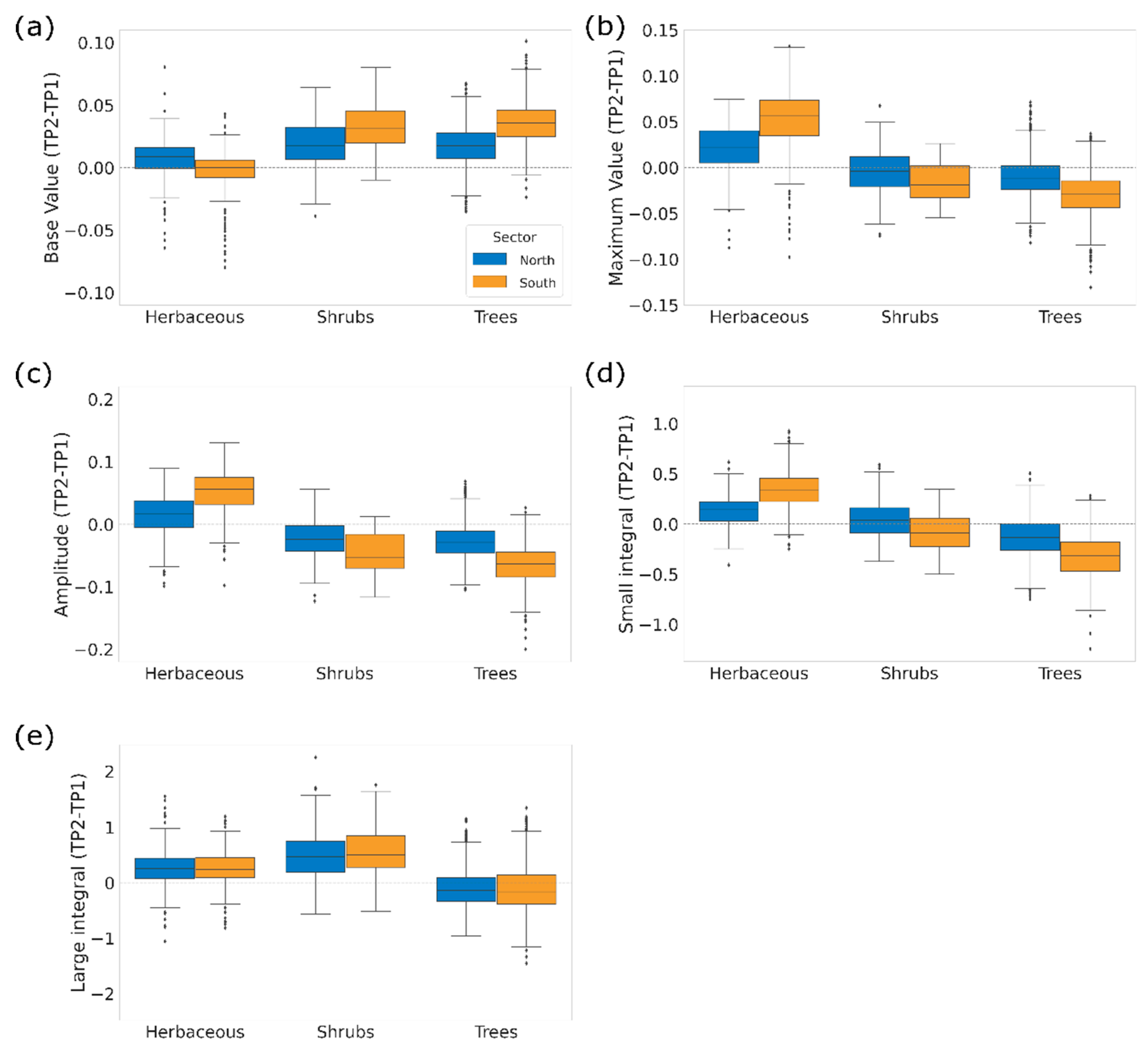
Starting with the herbaceous cover, the time-series shows a productivity increase in both sectors (associated with the maximum NDVI value) which contributed to raise the amplitude, as well as the value of the small and large integral. However, large effect sizes were only found for the maximum NDVI and for the small integral (associated with the seasonal productivity) in the south sector (Table 3 and Table 4, Appendix A, Figure A4). The comparison of changes between sectors supports this result, revealing larger differences in the south sector (Table 5, Figure 4). Moreover, because sectors show similar changes in the value of the large integral, but differ in the response of the small integral, the increase in the productivity of herbs during the growing season appears to be promoted by the introduction of cattle grazing.
In the shrub-covered areas, changes in productivity metrics were associated with an increase in the base value and a consequent decrease in amplitude in both sectors (Table 3 and Table 4, Appendix A, Figure A4). However, the rise of the base value is probably related to the signal of the herbaceous layer in autumn/winter, being that this a time of low seasonal productivity for shrubs. Effect sizes comparing changes between sectors are relatively small for all metrics, which reinforces the inference that this result is driven by the signal of herbaceous cover and not a real change in shrub productivity dynamics. Moreover, the increase in the value of the large integral (observed and equivalent in both sectors) is likely a consequence of the expansion of shrub cover during the study period and not necessarily of an increased productivity during the growing season (changes in the small integral were not significant). Nevertheless, it is worth noting that, at the peak season, the productivity of shrubs shows a decline in season 4 (Figure 2), with potential effects on the value of the large integral.
Finally, in tree dominated areas, the main changes in productivity metrics were an increase in the base value and a decrease in the amplitude, which were observed in both sectors, but with stronger effects on the south sector (Table 3 and Table 4, Appendix A, Figure A4). As for shrubs, this result is likely caused by the signal of the herbaceous layer, especially because trees are leafless at their base value, and herbs have started their growing season, and because the effect is stronger in the south sector (Table 5, Figure 4), where the herbaceous layer showed an increased productivity after the introduction of cattle grazing. Moreover, the decrease in amplitude in the south sector also seems to be due to a decrease in maximum productivity, which was observed in both sectors but more pronouncedly in the south sector (Table 5, Figure 4).

4. Discussion

This study analyzed the potential of remotely sensed satellite data to characterize vegetation phenology and productivity patterns and to detect changes driven by grazing disturbance in a heterogenous Mediterranean deciduous forest. Due to the expected differences in the phenological dynamics of the main vegetation types (i.e., herbs, shrubs and trees) and in their responses to grazing, landcover data were disaggregated before data analysis and vegetation types were examined independently.
More specifically, the combined used of a high-resolution landcover map (20 cm pixel; produced from drone imagery) with a time-series of high-resolution satellite data (10 m pixel) made possible the identification of relatively homogenous landcover patches within the forest mosaic, as well as the characterization of each vegetation type. This approach enabled a more comprehensive assessment of the seasonal dynamics in play. Moreover, because the study followed two contiguous areas that shared equivalent edaphoclimatic conditions, the specific responses of vegetation to livestock grazing could be singled out from the responses to other factors of change by means of a BACI experimental design, which facilitated the identification of the most responsive vegetation seasonal metrics and is an important contribution to future research on this subject and to the development of effective monitoring protocols supported by informative indicators. Furthermore, grazing-driven changes were detectable at an early stage of the grazing intervention, which reinforces the potential of satellite-based phenological time-series to monitor the use of livestock grazing for ecosystem management in fine-grained landscape mosaics and to foster adaptive management approaches.

4.1. Vegetation Seasonal Dynamics and Response to Grazing

The phenological curves here presented are consistent with the overall regional patterns described for the Iberian Peninsula [41] and show the distinct nature of each vegetation type. More specifically, the analyzed vegetation types show a time lag at the start of the growing season, with the herbaceous layer starting first in the autumn, followed by shrubs in the winter, and finally by deciduous trees in early spring (Figure 2, Table 2). There are also differences between the base and maximum NDVI values and consequently in amplitude. Being perennial, shrubs show lower NDVI amplitudes, with moderate values of minimum and maximum NDVI. Both trees and herbs show low base values (trees are leafless in winter, and herbs are senescent in summer) and moderate values, in the case of herbs, or high values, in the case of trees, of maximum NDVI, with the peak being reached around March by herbs and in May/June by trees.
The characterization of the main phenological dynamics present in a Pyrenean oak forest provides a valuable benchmark against which to monitor the trajectories of change in vegetation phenology and productivity in this type of ecosystem at a fine spatial scale. Due to the fact that this study is circumscribed to an area of approximately 200 ha, the generalization of these findings to the regional scale, which encompasses a larger diversity of environmental conditions, requires additional studies based on an unbiased and regionally representative sample [42]. Despite this caveat, we consider the patterns here described to be representative of the main dynamics present in the transitional landscapes found in the region, that is, landscapes under secondary succession following abandonment and/or large-scale disturbance events, namely fire, where vegetation types (trees, shrubs, and herbaceous patches) co-occur and are interspersed. Moreover, the use of high resolution spatial data is an important step to address the limitations of coarse spatial data when applied to the monitoring of heterogenous landscapes [43,44], including the failure to capture nuanced vegetation responses and effectively monitor changes to inform the best management decisions. Coarse resolution landcover maps produced at the national or regional scales, such as Corine Land Cover maps (https://land.copernicus.eu/), are often used as ancillary data to delimit the different landcover units, namely forest patches. However, these map products, which are produced for large spatial extents, ignore the fine-scale structure of vegetation within patches and inter-patch variability, thus missing an important component of ecosystem functioning when studying local-to-landscape scale processes [45]. In this study, the access to a high-resolution landcover map was critical to overcome such challenges and to enable a fine scale analysis that accounted for the structural heterogeneity of the forest patch that otherwise would only have been characterized by its shape and size and treated as structurally uniform. Hence, the method here described is particularly suited to monitor specific vegetation’s responses to management in fine-grained vegetation mosaics composed of multiple vegetation types but sharing similar edaphoclimatic conditions on the landscape scale.
Regarding the concrete responses to grazing, herbaceous vegetation was the most responsive, showing both phenology and productivity changes in the first years after the start of the grazing intervention. This result was expected, not only because this type of vegetation is the most subject to livestock grazing, but also because of the species’ short-term life cycles (annual, biennial), which allows a faster response to drivers of change. After the introduction of cattle in the south sector, seasonal events, namely the peak season time and the end of the growing season, suffered an anticipation. This change was possibly promoted by the lower amount of accumulated senescent herbaceous biomass in autumn (due to previous grazing and biomass removal), which enhanced the conditions for seed germination and seedling emergence in early autumn, namely more access to sunlight and space, when the abiotic conditions became appropriate for the start of the herb’s growing season [26]. This change was also accompanied by an increase in biomass production, revealed by a higher NDVI value at the season peak, which is a proxy for the maximum level of productivity, and a higher value of the small integer, which is an indicator of seasonal biomass production. Light to moderate grazing has been identified as a driver of grassland productivity, especially in areas where herbivores and plant communities evolved together [46]. The moderate disturbance effect created by herbivore presence has been associated with the maintenance of light and space availability, as well as with the control of dominant species, which may ultimately contribute to increased productivity by fostering plant-niche complementarity during the growing season [28,47].
Unlike the herbaceous layer, shrubs and trees did not show significant changes, driven by grazing, in phenological metrics but results suggest changes in productivity metrics. In the case of shrubs, the shape of the phenology curve (Figure 2) shows a flattening of the maximum NDVI values in the grazed sector in the last growing season (season 4), which suggests a decline in the overall productivity of the shrub layer. This change was not captured by statistical testing, which compared the average of the first two seasons with the average of the last two seasons but is probably related to the effect of trampling and herbivory by cattle. Trees showed a decrease in overall productivity in both the ungrazed and the grazed sectors; however, the change was more pronounced in the grazed sector. This trend is particularly reflected by the decline in the maximum NDVI value (Figure 2 and Figure 4), which is an indicator of lower tree productivity at the peak season. On the other hand, the decline in the value of the small integer is both linked to the decline in the maximum NDVI and to the increase in the base value (associated with the higher productivity of the herbaceous layer in the winter).
When compared to the north sector, the south sector was already characterized (in seasons 1 and 2, Table 1 and Figure 2) by a lower seasonal productivity, as indicated by the lower values of the maximum NDVI and of the small integer (with similar base values). This condition could be related to the effect of former fires and a higher level of fragmentation of tree cover in the south sector, which may have eroded the resilience of trees to the pressure exerted by climatic variability and grazing. While the relative contribution of each cause to the potential decline in primary productivity needs to be further investigated in future research, the current finding calls for targeted monitoring to avoid the unintended effects of cattle grazing in the condition of trees.

4.2. Use of NDVI Time-Series to Monitor Grazing

This study demonstrates the potential of NDVI time-series to monitor grazing effects on vegetation in fine-grained landscape mosaics and, particularly, to monitor grazing interventions for ecosystem restoration. All vegetation types exhibited changes in vegetation phenology or productivity that could be related to grazing. Moreover, these changes were already detectable by remote sensing after two growing seasons, which further supports the value of this type of data in fine-scale, large-extent, and continuous monitoring approaches.
The separate analysis by vegetation type shows that the suitability of vegetation metrics as indicators of change depends on the type of vegetation and on its responsiveness to the driver of change. In the case of herbaceous vegetation, both phenology and productivity indicators were useful to characterize the changes driven by the implementation of grazing. Notably, there were changes in the time of maximum productivity and in the magnitude of productivity (indicated by maximum NDVI and by the small integral) which are relevant to guide management, such as evaluating the system carrying capacity to keep grazing within sustainable limits [16,17,19]. For woody vegetation, that is, perennial shrubs and deciduous trees, only the productivity metrics seemed to change after grazing disturbance, at least in the first two seasons after livestock introduction. In this case, changes in the maximum NDVI value signaled a potential loss of productivity in the peak season. In the context of our case study, the decline in shrub productivity could be interpreted as a positive outcome, suggesting that the overall shrub biomass is being controlled and reduced by livestock disturbance, while in the case of trees it can be an early signal of unintended impacts and of the need to take action to mitigate them.
Moreover, some of the observed changes in productivity metrics in areas dominated by shrubs or trees were likely related to changes in the herbaceous layer. That is the case of the detected increase in the base NDVI value (with cascading effects on other metrics, such as amplitude and the small integral) at a time when shrubs are at minimum productivity levels and trees are leafless. In both cases, the relative contribution of the herbaceous layer to the overall signal of the vegetation is expected to be larger at that seasonal time and influence the observed NDVI value. Hence, while the current approach was successful in disaggregating the main vegetation types from a horizontal (aerial) structure perspective it has limitations regarding signal interferences from vertical stratification. In those cases, being aware of the distinct phenology of each vegetation type is an important step to disentangle responses, discard unclear results or eventually decide on the need of complementary approaches to confirm or refine results. The challenges posed by vertical stratification could also be addressed by monitoring the different vegetation types at different times in the year [43,48], as a complementary approach, or using data obtained from LiDAR (Light Detection and Ranging) or SAR (Synthetic Aperture Radar) sensors to characterize the composition of vegetation layers at each point [49]. However, the use of these type of data is still constrained by data availability and by technical capacity, which require advanced technical skills for data processing and interpretation [49,50].
Furthermore, while some metrics are potentially more informative than others, it is important to take all metrics into consideration when investigating vegetation changes [44], as they represent different aspects of the same response to a driver, or drivers, of change. For instance, an increase in the value of the large integral of perennial vegetation, as observed for shrubs (Table 3 and Table 4), that is not accompanied by an increase of the small integral, may indicate an accumulation of biomass from one year to the next, instead of an increase in seasonal productivity. Similarly, a decline in the small integral that is associated with a spurious increase of the base value, as observed for trees (Table 4 and Table 5), should also be interpreted with caution.
In summary, there is always the risk in stratified environments of signal interference by the understory layers, especially when the top layers are characterized by a sparse cover or are in a deciduous stage. Metrics that depend on other metrics are more vulnerable to this effect; that is the case of metrics dependent on the base value, such as amplitude and the small integral. On the other hand, metrics such as the maximum NDVI seem to be of less concern, especially if the areas selected for the study are characterized by a relatively homogenous cover of the dominant vegetation type. In our study, the selection of the pixels that would represent each vegetation type followed rules to ensure a homogenous cover at the pixel level, at least at the time of their maximum productivity. We found seasonal timing, or phenology metrics, to be less prone to signal contamination from vegetation types other than dominant type.
Finally, the overall set of metrics indicating changes in vegetation phenology and productivity is more diverse than the particular set of metrics responding to grazing. In this study, several metrics reflected the changes associated with the ongoing trajectory of vegetation succession and driven by natural climatic variability (Table 3 and Table 4), being, therefore, relevant for baseline monitoring purposes. Moreover, while this study delivers promising results on the potential of using NDVI time-series to monitor grazing on the landscape scale, future research should consider and evaluate the performance of multiple vegetation indexes (e.g., EVI, GNDVI) and of spectral band combinations to monitor the different vegetation types and in different landscape configurations, because the performance will depend on the context of application [51].

5. Conclusions

In this study, the challenges posed by the fine-grained structure (horizontal heterogeneity) of the landscape mosaic were mitigated by the intersection of the Sentinel-2 grid with an updated high-resolution landcover map of the study area and by using a conservative approach to select pixels that were representative of the different landcover types. The methods tested here demonstrate the potential of using satellite data to monitor vegetation changes in fine-grained landscape mosaics and, in particular, to monitor the effect of grazing, which is critical for ensuring sustainable grazing regimes or monitoring the use of livestock grazing in ecosystem restoration. On the other hand, the challenges posed by vertical stratification call for further research into complementary methods and data types (e.g., LiDAR data) that may help to overcome these challenges, especially when working on structurally complex areas composed of several vegetation layers. Nevertheless, a good knowledge of the phenological baseline dynamics of each vegetation type is essential to decouple the relative contribution of their signals from the overall reflectance of the vegetation and be able to critically interpret the extracted phenology and productivity metrics.
This study was successful in describing the seasonal dynamics of the main vegetation types in a deciduous oak forest mosaic with a fined-grained vegetation structure. Moreover, it captured the effects of grazing in vegetation seasonal metrics. In particular, the implementation of extensive (low-intensity) livestock grazing so far appears to be promoting an increase in the productivity of herbaceous vegetation and an anticipation of the peak season. Other effects that can be inferred from the data, although with less certainty, are a restraining effect on shrub productivity in peak season and a similar, but unintended, effect on tree productivity.
Finally, our findings suggest that the indicator value of seasonal metrics depends on the type of vegetation being monitored, an aspect that should be considered when designing monitoring protocols. In our case, we found that at an early stage of the grazing intervention (circa three years since the start) productivity metrics were more responsive than phenology metrics in the case of woody vegetation, while both types of metrics were responsive in the case of herbaceous vegetation.

Author Contributions

Conceptualization, D.B. and V.P.; Methodology, D.B., I.G. and V.P.; Software, D.B.; Formal Analysis, D.B.; Resources, I.G.; Writing—Original Draft Preparation, D.B. and V.P.; Writing—Review and Editing, T.D. and V.P.; Supervision, V.P. All authors have read and agreed to the published version of the manuscript.

Funding

This research was funded by the projects “SILVPAST—Cost-efficient implementation of silvo-pastoral mosaic systems of black oak” (PDR2020-101-031873), SILVANUS (European Union’s Horizon 2020 Research and Innovation Program Grant Agreement no. 101037247), and by FCT/MCTES (PIDDAC) through project LARSyS—FCT Pluriannual funding 2020–2023 (UIDB/50009/2020) and CEECIND/04469/2017 (V. Proença).

Data Availability Statement

Not applicable.

Acknowledgments

The authors would like to thank the reviewers for their comments which contributed to improve the paper.

Conflicts of Interest

The authors declare no conflict of interest.

Appendix A

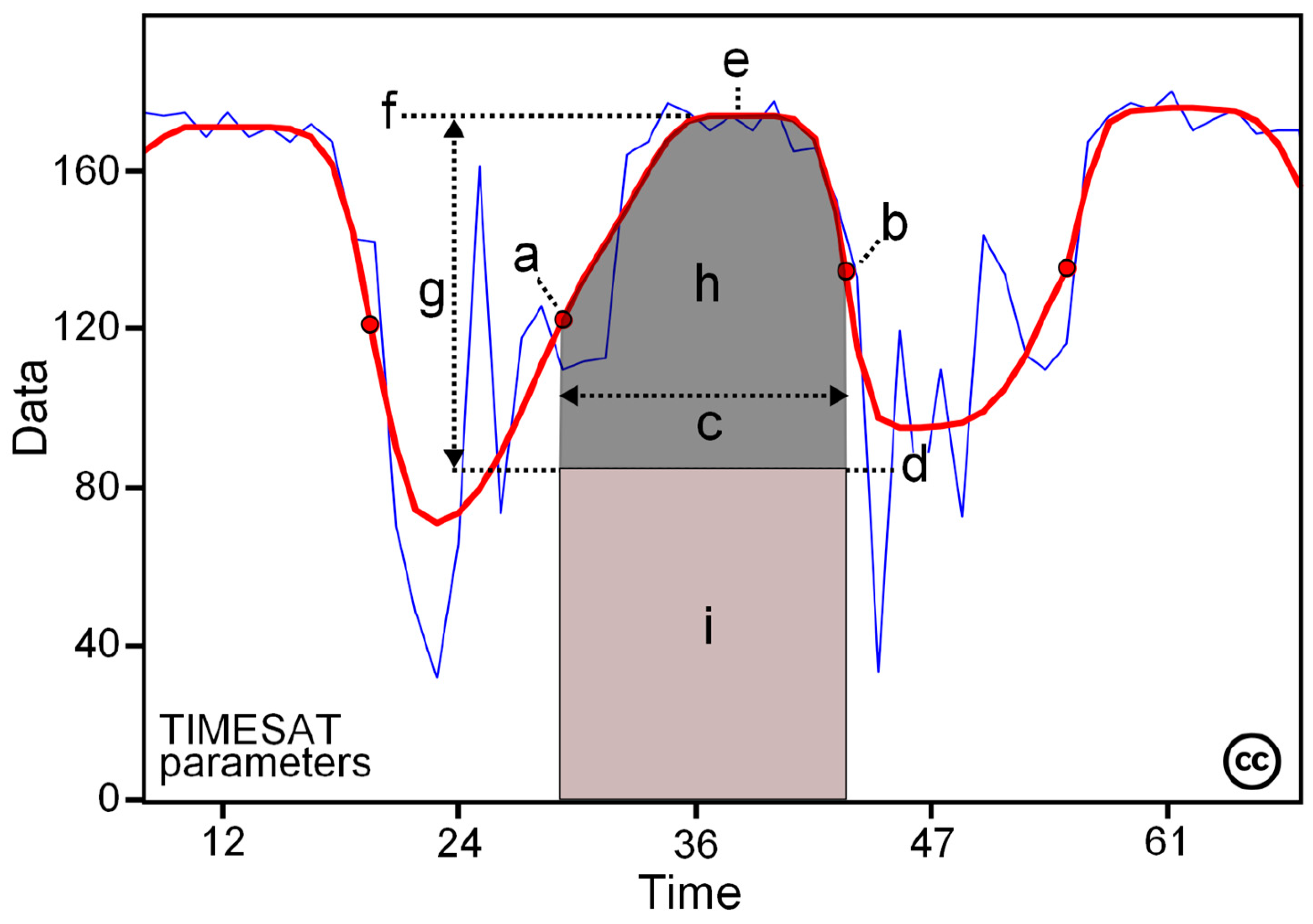
Figure A1. Some of the seasonality parameters generated in TIMESAT [24]: (a) beginning of season, (b) end of season, (c) length of season, (d) base value, (e) time of middle of season, (f) maximum value, (g) amplitude, and (h) small integrated value, (h + i) large integrated value. Raw time-series values are represented by the blue curve and the fitted time-series by the red curve. This figure is licensed under a Creative Commons Attribution-Non-Commercial-NoDerivs 2.5 Sweden License.
Remotesensing 14 02322 g0a1
Figure A2. Accumulated monthly precipitation (a) and monthly temperatures (b) for the region of Covilhã, Castelo Branco, Portugal from January 2016 to June 2021 (Source: https://www.worldweatheronline.com/covilha-weather-averages/castelo-branco/pt.aspx, accessed on 14 September 2021). Vertical gridlines indicate the first day of each year.
Remotesensing 14 02322 g0a2
Figure A3. Changes in phenological metrics during the study period. Median values are shown for (a) the start of the growing season, (b) maximum productivity and (c) season end for each type of vegetation in both sectors. The error bars depict the median absolute deviations.
Remotesensing 14 02322 g0a3
Figure A4. Changes in productivity metrics during the study period. Boxplots show the distribution of the values of the pixels averaged for the two seasons in each time interval (seasons 1–2 vs. seasons 3–4) for the metrics: (a) base value, (b) maximum value, (c) amplitude, (d) small integral, and (e) large integral.
Remotesensing 14 02322 g0a4

References

  1. Ripple, W.J.; Newsome, T.M.; Wolf, C.; Dirzo, R.; Everatt, K.T.; Galetti, M.; Hayward, M.W.; Kerley, G.I.H.; Levi, T.; Lindsey, P.A.; et al. Collapse of the World’s Largest Herbivores. Sci. Adv. 2015, 1, e1400103. [Google Scholar] [CrossRef] [PubMed] [Green Version]
  2. Smit, C.; Putman, R. Large Herbivores as ‘Environmental Engineers’. In Ungulate Management in Europe: Problems and Practices; Apollonio, M., Andersen, R., Putman, R., Eds.; Cambridge University Press: Cambridge, UK, 2011; pp. 260–283. ISBN 978-0-521-76059-1. [Google Scholar]
  3. Teillard, F.; de Souza, D.M.; Thoma, G.; Gerber, P.J.; Finn, J.A. What Does Life-Cycle Assessment of Agricultural Products Need for More Meaningful Inclusion of Biodiversity? J. Appl. Ecol. 2016, 53, 1422–1429. [Google Scholar] [CrossRef] [Green Version]
  4. Bignal, E.; McCracken, D. The Conservation Value of European Traditional Farming Systems. Environ. Rev. 2000, 8, 149–171. [Google Scholar] [CrossRef]
  5. Navarro, L.M.; Proença, V.; Kaplan, J.O.; Pereira, H.M. Maintaining Disturbance-Dependent Habitats. In Rewilding European Landscapes; Pereira, H.M., Navarro, L.M., Eds.; Springer International Publishing: Cham, Switzerland, 2015; pp. 143–167. ISBN 978-3-319-12039-3. [Google Scholar]
  6. Fernández-Manjarrés, J.F.; Ruiz-Benito, P.; Zavala, M.A.; Camarero, J.J.; Pulido, F.; Proença, V.; Navarro, L.; Sansilvestri, R.; Granda, E.; Marqués, L.; et al. Forest Adaptation to Climate Change along Steep Ecological Gradients: The Case of the Mediterranean-Temperate Transition in South-Western Europe. Sustainability 2018, 10, 3065. [Google Scholar] [CrossRef] [Green Version]
  7. Honrado, J.P.; Lomba, A.; Alves, P.J.M.; Aguiar, C.; Monteiro-Henriques, T.; Cerqueira, Y.; Monteiro, P.; Caldas, F.B. Conservation Management of EU Priority Habitats after Collapse of Traditional Pastoralism: Navigating Socioecological Transitions in Mountain Rangeland. Rural Sociol. 2017, 82, 101–128. [Google Scholar] [CrossRef] [Green Version]
  8. Lomba, A.; Moreira, F.; Klimek, S.; Jongman, R.H.; Sullivan, C.; Moran, J.; Poux, X.; Honrado, J.P.; Pinto-Correia, T.; Plieninger, T.; et al. Back to the Future: Rethinking Socioecological Systems Underlying High Nature Value Farmlands. Front. Ecol. Environ. 2020, 18, 36–42. [Google Scholar] [CrossRef]
  9. Navarro, L.M.; Marques, A.; Proença, V.; Ceauşu, S.; Gonçalves, B.; Capinha, C.; Fernandez, M.; Geldmann, J.; Pereira, H.M. Restoring Degraded Land: Contributing to Aichi Targets 14, 15, and Beyond. Curr. Opin. Environ. Sustain. 2017, 29, 207–214. [Google Scholar] [CrossRef]
  10. Gordon, I.J.; Manning, A.D.; Navarro, L.M.; Rouet-Leduc, J. Domestic Livestock and Rewilding: Are They Mutually Exclusive? Front. Sustain. Food Syst. 2021, 5, 550410. [Google Scholar] [CrossRef]
  11. Ruiz-Mirazo, J.; Robles, A.; González-Rebollar, J. Two-Year Evaluation of Fuelbreaks Grazed by Livestock in the Wildfire Prevention Program in Andalusia (Spain). Agric. Ecosyst. Environ. 2011, 141, 13–22. [Google Scholar] [CrossRef]
  12. Vermeulen, R. (Ed.) Natural Grazing—Practices in the Rewilding of Cattle and Horses; Rewilding Europe: Nijmegen, The Netherlands, 2015; p. 40. [Google Scholar]
  13. Franzluebbers, A.J.; Paine, L.K.; Winsten, J.R.; Krome, M.; Sanderson, M.A.; Ogles, K.; Thompson, D. Well-Managed Grazing Systems: A Forgotten Hero of Conservation. J. Soil Water Conserv. 2012, 67, 100A–104A. [Google Scholar] [CrossRef] [Green Version]
  14. Lunt, I.D.; Eldridge, D.J.; Morgan, J.W.; Witt, G.B.; Lunt, I.D.; Eldridge, D.J.; Morgan, J.W.; Witt, G.B. A Framework to Predict the Effects of Livestock Grazing and Grazing Exclusion on Conservation Values in Natural Ecosystems in Australia. Aust. J. Bot. 2007, 55, 401–415. [Google Scholar] [CrossRef]
  15. Kristensen, J.A.; Svenning, J.-C.; Georgiou, K.; Malhi, Y. Can Large Herbivores Enhance Ecosystem Carbon Persistence? Trends Ecol. Evol. 2022, 37, 117–128. [Google Scholar] [CrossRef] [PubMed]
  16. Papanastasis, V. Restoration of Degraded Grazing Lands through Grazing Management: Can It Work? Restor. Ecol. 2009, 17, 441–445. [Google Scholar] [CrossRef]
  17. Giralt-Rueda, J.M.; Santamaria, L. Complementary Differences in Primary Production and Phenology among Vegetation Types Increase Ecosystem Resilience to Climate Change and Grazing Pressure in an Iconic Mediterranean Ecosystem. Remote Sens. 2021, 13, 3920. [Google Scholar] [CrossRef]
  18. Sánchez-Cuesta, R.; Ruiz-Gómez, F.J.; Duque-Lazo, J.; González-Moreno, P.; Navarro-Cerrillo, R.M. The Environmental Drivers Influencing Spatio-Temporal Dynamics of Oak Defoliation and Mortality in Dehesas of Southern Spain. For. Ecol. Manag. 2021, 485, 118946. [Google Scholar] [CrossRef]
  19. von Keyserlingk, J.; de Hoop, M.; Mayor, A.G.; Dekker, S.C.; Rietkerk, M.; Foerster, S. Resilience of Vegetation to Drought: Studying the Effect of Grazing in a Mediterranean Rangeland Using Satellite Time Series. Remote Sens. Environ. 2021, 255, 112270. [Google Scholar] [CrossRef]
  20. Bégué, A.; Arvor, D.; Lelong, C.; Vintrou, E.; Simoes, M. Agricultural Systems Studies Using Remote Sensing. In Remote Sensing Handbook, Vol. 2: Land Resources Monitoring, Modeling, and Mapping with Remote Sensing; CRC Press: Boca Raton, FL, USA, 2015. [Google Scholar]
  21. Skidmore, A. Remote Sensing of EBVs for Global Change Monitoring. In Proceedings of the Global Change and Biodiversity: Integrating Mechanisms of Interactions, Feedbacks and Scale: URPP Global Change and Biodiversity Conference: Program and Abstract Book, Ascona, Switzerland, 28 August–1 September 2016. [Google Scholar]
  22. Tian, X.; Minunno, F.; Schiestl-Aalto, P.; Chi, J.; Zhao, P.; Peichl, M.; Marshall, J.; Näsholm, T.; Lim, H.; Peltoniemi, M.; et al. Disaggregating the Effects of Nitrogen Addition on Gross Primary Production in a Boreal Scots Pine Forest. Agric. For. Meteorol. 2021, 301–302, 108337. [Google Scholar] [CrossRef]
  23. Pettorelli, N.; Vik, J.O.; Mysterud, A.; Gaillard, J.-M.; Tucker, C.J.; Stenseth, N.C. Using the Satellite-Derived NDVI to Assess Ecological Responses to Environmental Change. Trends Ecol. Evol. 2005, 20, 503–510. [Google Scholar] [CrossRef]
  24. Jönsson, P.; Eklundh, L. TIMESAT—A Program for Analyzing Time-Series of Satellite Sensor Data. Comput. Geosci. 2004, 30, 833–845. [Google Scholar] [CrossRef] [Green Version]
  25. Davis, C.L.; Hoffman, M.T.; Roberts, W. Long-term trends in vegetation phenology and productivity over Namaqualand using the GIMMS AVHRR NDVI3g data from 1982 to 2011. S. Afr. J. Bot. 2017, 111, 76–85. [Google Scholar] [CrossRef]
  26. Knapp, A.K.; Hoover, D.L.; Blair, J.M.; Buis, G.; Burkepile, D.E.; Chamberlain, A.; Collins, S.L.; Fynn, R.W.S.; Kirkman, K.P.; Smith, M.D.; et al. A Test of Two Mechanisms Proposed to Optimize Grassland Aboveground Primary Productivity in Response to Grazing. J. Plant Ecol. 2012, 5, 357–365. [Google Scholar] [CrossRef] [Green Version]
  27. Papoutsa, C.; Kouhartsiouk, D.; Themistocleous, K.; Christoforou, M.; Hadjimitsis, D.G. Monitoring of Land Degradation from Overgrazing Using Space-Borne Radar and Optical Imagery: A Case Study in Randi Forest, Cyprus; Michel, U., Schulz, K., Ehlers, M., Nikolakopoulos, K.G., Civco, D., Eds.; SPIE: Edinburgh, UK, 2016; p. 1000516. [Google Scholar]
  28. Charles, G.K.; Porensky, L.M.; Riginos, C.; Veblen, K.E.; Young, T.P. Herbivore Effects on Productivity Vary by Guild: Cattle Increase Mean Productivity While Wildlife Reduce Variability. Ecol. Appl. 2017, 27, 143–155. [Google Scholar] [CrossRef] [PubMed] [Green Version]
  29. Christie, A.P.; Amano, T.; Martin, P.A.; Shackelford, G.E.; Simmons, B.I.; Sutherland, W.J. Simple Study Designs in Ecology Produce Inaccurate Estimates of Biodiversity Responses. J. Appl. Ecol. 2019, 56, 2742–2754. [Google Scholar] [CrossRef] [Green Version]
  30. Ockendon, N.; Amano, T.; Cadotte, M.; Downey, H.; Hancock, M.H.; Thornton, A.; Tinsley-Marshall, P.; Sutherland, W.J. Effectively Integrating Experiments into Conservation Practice. Ecol. Solut. Evid. 2021, 2, e12069. [Google Scholar] [CrossRef]
  31. D’Odorico, P.; Gonsamo, A.; Damm, A.; Schaepman, M.E. Experimental Evaluation of Sentinel-2 Spectral Response Functions for NDVI Time-Series Continuity. IEEE Trans. Geosci. Remote Sens. 2013, 51, 1336–1348. [Google Scholar] [CrossRef]
  32. Tucker, C.J. Red and Photographic Infrared Linear Combinations for Monitoring Vegetation. Remote Sens. Environ. 1979, 8, 127–150. [Google Scholar] [CrossRef] [Green Version]
  33. Jiang, Z.; Huete, A.R.; Chen, J.; Chen, Y.; Li, J.; Yan, G.; Zhang, X. Analysis of NDVI and Scaled Difference Vegetation Index Retrievals of Vegetation Fraction. Remote Sens. Environ. 2006, 101, 366–378. [Google Scholar] [CrossRef]
  34. Hmimina, G.; Dufrêne, E.; Pontailler, J.-Y.; Delpierre, N.; Aubinet, M.; Caquet, B.; de Grandcourt, A.; Burban, B.; Flechard, C.; Granier, A.; et al. Evaluation of the Potential of MODIS Satellite Data to Predict Vegetation Phenology in Different Biomes: An Investigation Using Ground-Based NDVI Measurements. Remote Sens. Environ. 2013, 132, 145–158. [Google Scholar] [CrossRef]
  35. Pan, Z.; Huang, J.; Zhou, Q.; Wang, L.; Cheng, Y.; Zhang, H.; Blackburn, G.A.; Yan, J.; Liu, J. Mapping Crop Phenology Using NDVI Time-Series Derived from HJ-1 A/B Data. Int. J. Appl. Earth Obs. Geoinf. 2015, 34, 188–197. [Google Scholar] [CrossRef] [Green Version]
  36. Weber, D.; Schaepman-Strub, G.; Ecker, K. Predicting Habitat Quality of Protected Dry Grasslands Using Landsat NDVI Phenology. Ecol. Indic. 2018, 91, 447–460. [Google Scholar] [CrossRef]
  37. Lin, M.; Lucas, H.C.; Shmueli, G. Research Commentary—Too Big to Fail: Large Samples and the p-Value Problem. Inf. Syst. Res. 2013, 24, 906–917. [Google Scholar] [CrossRef] [Green Version]
  38. Sullivan, G.M.; Feinn, R. Using Effect Size—or Why the P Value Is Not Enough. J. Grad. Med. Educ. 2012, 4, 279–282. [Google Scholar] [CrossRef] [PubMed] [Green Version]
  39. Cliff, N. Answering Ordinal Questions with Ordinal Data Using Ordinal Statistics. Multivar. Behav. Res. 1996, 31, 331–350. [Google Scholar] [CrossRef] [PubMed]
  40. Romano, J.; Kromrey, J. Appropriate Statistics for Ordinal Level Data: Should We Really Be Using t-Test and Cohen’s d for Evaluating Group Differences on the NSSE and Other Surveys? In Proceedings of the Annual Meeting of the Florida Association of Institutional Research; Florida Association for Institutional Research: Cocoa Beach, FL, USA, 2006. [Google Scholar]
  41. Alcaraz-Segura, D.; Cabello, J.; Paruelo, J. Baseline Characterization of Major Iberian Vegetation Types Based on the NDVI Dynamics. Plant Ecol. 2009, 202, 13–29. [Google Scholar] [CrossRef]
  42. Olofsson, P.; Foody, G.M.; Herold, M.; Stehman, S.V.; Woodcock, C.E.; Wulder, M.A. Good practices for estimating area and assessing accuracy of land change. Remote Sens. Environ. 2014, 148, 42–57. [Google Scholar] [CrossRef]
  43. Kuemmerle, T.; Röder, A.; Hill, J. Separating Grassland and Shrub Vegetation by Multidate Pixel-adaptive Spectral Mixture Analysis. Int. J. Remote Sens. 2006, 27, 3251–3271. [Google Scholar] [CrossRef]
  44. Walker, J.J.; Soulard, C.E. Phenology Patterns Indicate Recovery Trajectories of Ponderosa Pine Forests After High-Severity Fires. Remote Sens. 2019, 11, 2782. [Google Scholar] [CrossRef] [Green Version]
  45. Ribeiro, I.; Proença, V.; Serra, P.; Palma, J.; Domingo-Marimon, C.; Pons, X.; Domingos, T. Remotely Sensed Indicators and Open-Access Biodiversity Data to Assess Bird Diversity Patterns in Mediterranean Rural Landscapes. Sci. Rep. 2019, 9, 6826. [Google Scholar] [CrossRef] [Green Version]
  46. Forbes, E.S.; Cushman, J.H.; Burkepile, D.E.; Young, T.P.; Klope, M.; Young, H.S. Synthesizing the effects of large, wild herbivore exclusion on ecosystem function. Funct. Ecol. 2019, 33, 1597–1610. [Google Scholar] [CrossRef] [Green Version]
  47. Campana, S.; Tognetti, P.M.; Yahdjian, L. Livestock exclusion reduces the temporal stability of grassland productivity regardless of eutrophication. Sci. Total Environ. 2022, 817, 152707. [Google Scholar] [CrossRef]
  48. Helman, D.; Lensky, I.M.; Tessler, N.; Osem, Y. A phenology-based method for monitoring woody and herbaceous vegetation in Mediterranean forests from NDVI time series. Remote Sens. 2015, 7, 12314–12335. [Google Scholar] [CrossRef] [Green Version]
  49. Nagendra, H.; Lucas, R.; Honrado, J.P.; Jongman, R.H.; Tarantino, C.; Adamo, M.; Mairota, P. Remote sensing for conservation monitoring: Assessing protected areas, habitat extent, habitat condition, species diversity, and threats. Ecol. Indic. 2013, 33, 45–59. [Google Scholar] [CrossRef]
  50. Pettorelli, N.; Wegmann, M.; Skidmore, A.; Mucher, S.; Dawson, T.P.; Fernandez, M.; Lucas, R.; Schaepman, M.E.; Wang, T.; O’Connor, B.; et al. Framing the concept of satellite remote sensing essential biodiversity variables: Challenges and future directions. Remote Sens. Ecol. Conserv. 2016, 2, 122–131. [Google Scholar] [CrossRef]
  51. Chaves, M.E.D.; Picoli, M.C.A.; Sanches, I.D. Recent Applications of Landsat 8/OLI and Sentinel-2/MSI for Land Use and Land. Cover Mapping: A Systematic Review. Remote Sens. 2020, 12, 3062. [Google Scholar] [CrossRef]
Figure 1. (a) Location of Quinta da França in Portugal (40°17′1″N, 7°24′45″W); (b) Forest study area (colored) inside Quinta da França (black outer line), showing the two sectors separated by a fence: the north (control) in brown and the south (test) in blues. The area with more grazing is shown in darker blue; (c) High resolution landcover map overlapping the forest study area.
Remotesensing 14 02322 g001
Figure 2. Time-series of median and median absolute deviation (shaded areas) of NDVI in (a) herbaceous, (b) shrubs, and (c) tree-dominated areas. Vertical gridlines indicate the first day of each year, and the orange dot marks the start date (June 2018) of the grazing intervention in the south sector.
Remotesensing 14 02322 g002
Figure 3. Distribution of differences in phenology metrics between the two study periods for the pixels in each sector (north sector in blue, south sector in brown) and for each vegetation type. Positive values indicate a delay in the season start time (a), maximum time (b), and end time (c), or an increase in seasonal length (d) from the first two seasons to the last two seasons. Negative values indicate an anticipation or decrease, values close to zero indicate little or no change. TP1—Time Period 1 (seasons 1–2), TP2—Time Period 2 (seasons 3–4).
Remotesensing 14 02322 g003
Figure 4. Distribution of differences in productivity metrics between the two study periods for the pixels in each sector (north sector in blue, south sector in brown) and for each vegetation type. Positive values indicate an increase in base value (a), maximum value (b), amplitude (c), small integral (d), and large integral (e) from the first two seasons to the last two seasons. Negative values indicate a decrease, values close to zero indicate little or no change. TP1—Time Period 1 (seasons 1–2), TP2—Time Period 2 (seasons 3–4).
Remotesensing 14 02322 g004
Table 1. Definition of the phenology and productivity metrics used in this study [24,25].
Metric Definition
Phenology metrics
Season startPoint in time when NDVI reaches 20% of seasonal amplitude as measured from the left minimum level. It corresponds to the start of the growing season.
Season endPoint in time when NDVI reaches 20% of seasonal amplitude as measured from the right minimum level. It corresponds to the end of the growing season.
Season lengthLength of time from the start to the end of the season. It corresponds to the duration of the growing season
Time of maximum NDVI Date of the seasonal NDVI peak.
Productivity metrics
Base valueAverage of the left and right minimum values (between seasons).
Maximum valueLargest NDVI value for the fitted function during the season. A proxy of the maximum amount of vegetation for the sample point.
Seasonal amplitudeDifference between the maximum and base NDVI values for the season.
Small integralIntegral of the difference between the function describing the season and the base level from season start to end. Used as proxy for seasonal productivity between season start and season end.
Large integralIntegral of the function describing the season from start to end. Same as the small integral but with a cumulative start at zero NDVI. Used as a proxy for total productivity, including existing vegetation produced outside of growing season.
Table 2. Median values (and median absolute deviation) of the phenology and productivity metrics extracted from the TIMESAT fitted curve. Values are shown for the main vegetation types in each sector and for the first (Season 1–2) and second (Season 3–4) time intervals. Season start time (S start), season end time (S end), season length (S len), and the time of maximum NDVI (Max T) are measured in months (from 1 to 12, where a value of 1 corresponds with 1 January, and a value of 12 to 31 December). Seasonal base value (Base V), seasonal maximum value (Max V) and seasonal amplitude (Amp) correspond to NDVI values. Small Integral (S int) and large integral (L int) are the integrated values of the area under the NDVI curve.
ZoneSeasonS StartS EndS LenMax. TBase VMax VAmpS IntL Int
Herb. North1–210.91 (2.39)7.46 (1.73)8.41 (1.06)3.91 (2.13)0.23 (0.03)0.40 (0.05)0.17 (0.04)0.93 (0.18)3.19 (0.43)
3–410.88 (2.21)7.27 (1.94)8.42 (1.07)3.64 (2.01)0.24 (0.04)0.43 (0.04)0.19 (0.04)1.04 (0.23)3.54 (0.51)
Herb. South1–210.40 (1.87)7.21 (1.71)8.56 (0.84)3.21 (2.15)0.22 (0.03)0.38 (0.04)0.16 (0.03)0.91 (0.16)3.24 (0.35)
3–410.04 (1.44)6.60 (1.48)8.53 (0.57)2.25 (1.65)0.21 (0.03)0.42 (0.04)0.20 (0.05)1.16 (0.25)3.47 (0.32)
Shrubs North1–22.43 (1.99)9.27 (2.58)7.11 (1.40)5.34 (1.36)0.30 (0.03)0.53 (0.05)0.23 (0.05)1.06 (0.28)3.83 (0.67)
3–41.68 (1.92)10.26 (2.16)8.50 (0.84)5.44 (1.62)0.32 (0.03)0.53 (0.04)0.20 (0.04)1.09 (0.27)4.48 (0.52)
Shrubs South1–22.34 (2.66)8.24 (2.61)6.93 (1.75)5.12 (1.51)0.29 (0.03)0.48 (0.05)0.18 (0.04)0.82 (0.19)3.48 (0.71)
3–412.83 (2.70)8.47 (2.65)8.51 (1.21)4.96 (2.12)0.32 (0.03)0.46 (0.03)0.15 (0.03)0.79 (0.19)4.12 (0.56)
Trees North1–23.05 (1.16)11.86 (1.47)8.83 (0.43)6.07 (1.25)0.31 (0.03)0.70 (0.04)0.39 (0.05)2.25 (0.36)5.60 (0.43)
3–43.06 (1.45)11.28 (1.41)8.34 (0.46)6.61 (1.37)0.32 (0.03)0.68 (0.04)0.36 (0.05)2.11 (0.33)5.46 (0.40)
Trees South1–23.06 (1.24)11.78 (1.93)8.73 (0.82)5.84 (1.30)0.31 (0.02)0.67 (0.05)0.35 (0.05)1.92 (0.42)5.34 (0.59)
3–43.11 (1.64)11.15 (1.71)8.21 (0.56)6.40 (1.51)0.35 (0.03)0.63 (0.06)0.28 (0.03)1.59 (0.41)5.13 (0.45)
Table 3. Effect sizes (Cliff’s delta values, d) and Wilcoxon Signed-Rank test results of the changes in phenology and productivity metrics between the two time periods in the north sector. A positive delta value is associated with a delay in time, an increase in productivity metrics or in season length in the second time period (and vice-versa for negative values, see text). Wilcoxon Signed-Rank test p-values: ** p < 0.01, *** p < 0.001, n.s.: p > 0.05. Effect sizes are considered negligible if |d| < 0.147 and large (in bold) if |d| > 0.473.
North SectorHerbaceousShrubsTrees
Phenology metrics
Season startnegligible0.47 ***negligible
Season end−0.25 **negligible−0.66 ***
Season lengthn.s.0.43 ***−0.56 ***
Max. Time−0.23 ***0.27 ***0.80 ***
Productivity metrics
Base Valuen.s.0.35 ***0.34 ***
Max Value0.26 ***n.s.−0.19 ***
Amplitude0.16 ***−0.29 ***−0.34 ***
Small int.0.32 ***n.s.−0.25 ***
Large int.0.40 ***0.45 ***−0.18 ***
Table 4. Effect sizes (Cliff’s delta values, d) and Wilcoxon Signed-Rank test results of the changes in phenology and productivity metrics between the two time periods in the south sector. A positive delta value is associated with delay in time, an increase in productivity metrics or in season length in the second time period (and vice-versa for negative values, see text). Wilcoxon Signed-Rank test p-values: ** p < 0.01, *** p < 0.001, n.s.: p > 0.05. Effect sizes are considered negligible if |d| < 0.147 and large (in bold) if |d| > 0.473.
South SectorHerbaceousShrubsTrees
Phenology metrics
Season start−0.2 ***−0.40 ***n.s.
Season end−0.59 ***negligible−0.39 ***
Season lengthnegligible0.41 **−0.37 ***
Max. Time−0.65 ***negligible0.70 ***
Productivity metrics
Base Valuen.s.0.47 ***0.65 ***
Max Value0.50 ***−0.22 ***−0.32 ***
Amplitude0.27 *** −0.60 ***−0.55 ***
Small int.0.60 ***negligible−0.41 ***
Large int.0.40 ***0.49 ***negligible
Table 5. Effect sizes (Cliff’s delta values, d) and Mann-Whitney U test results comparing the magnitude of the temporal changes observed in the north and the south sectors. High positive delta values indicate a higher magnitude of change in the south sector when compared with the north sector (and vice-versa for negative values, see text). Mann-Whitney U test p-values: ** p < 0.01, *** p < 0.001, n.s. p > 0.05. Effect sizes under 0.147 are considered negligible. Effect sizes are considered negligible if |d| < 0.147 and large (in bold) if |d| > 0.473.
HerbaceousShrubsTrees
Phenology metrics
Season startnegligiblen.s.negligible
Season end0.45 ***n.s.negligible
Season length−0.18 ***n.s.negligible
Max. Time0.74 ***0.27 ***negligible
Productivity metrics
Base Value−0.20 ***0.33 ***0.58 ***
Max Value0.61 ***0.16 **0.44 ***
Amplitude0.55 ***0.32 ***0.63 ***
Small int.0.60 *** negligible 0.46 ***
Large int.n.s.n.s.n.s.
Publisher’s Note: MDPI stays neutral with regard to jurisdictional claims in published maps and institutional affiliations.