Article

A Random Forest Algorithm for Retrieving Canopy Chlorophyll Content of Wheat and Soybean Trained with PROSAIL Simulations Using Adjusted Average Leaf Angle

1
Key Laboratory of Digital Earth Science, Aerospace Information Research Institute, Chinese Academy of Sciences, Beijing 100094, China
2
College of Surveying and Planning, Shangqiu Normal University, Shangqiu 476000, China
3
China Remote Sensing Satellite Ground Station, Aerospace Information Research Institute, Chinese Academy of Sciences, Beijing 100094, China
4
University of Chinese Academy of Sciences, Beijing 100049, China
*
Author to whom correspondence should be addressed.
Remote Sens. 2022, 14(1), 98; https://doi.org/10.3390/rs14010098
Submission received: 29 November 2021 / Revised: 18 December 2021 / Accepted: 24 December 2021 / Published: 25 December 2021

Abstract

:
Canopy chlorophyll content (CCC) is an important indicator for crop-growth monitoring and crop productivity estimation. The hybrid method, involving the PROSAIL radiative transfer model and machine learning algorithms, has been widely applied for crop CCC retrieval. However, PROSAIL’s homogeneous canopy hypothesis limits the ability to use the PROSAIL-based CCC estimation across different crops with a row structure. In addition to leaf area index (LAI), average leaf angle (ALA) is the most important canopy structure factor in the PROSAIL model. Under the same LAI, adjustment of the ALA can make a PROSAIL simulation obtain the same canopy gap as the heterogeneous canopy at a specific observation angle. Therefore, parameterization of an adjusted ALA (ALAadj) is an optimal choice to make the PROSAIL model suitable for specific row-planted crops. This paper attempted to improve PROSAIL-based CCC retrieval for different crops, using a random forest algorithm, by introducing the prior knowledge of crop-specific ALAadj. Based on the field reflectance spectrum at nadir, leaf area index, and leaf chlorophyll content, parameterization of the ALAadj in the PROSAIL model for wheat and soybean was carried out. An algorithm integrating the random forest and PROSAIL simulations with prior ALAadj information was developed for wheat and soybean CCC retrieval. Ground-measured CCC measurements were used to validate the CCC retrieved from canopy spectra. The results showed that the ALAadj values (62 degrees for wheat; 45 degrees for soybean) that were parameterized for the PROSAIL model demonstrated good discrimination between the two crops. The proposed algorithm improved the CCC retrieval accuracy for wheat and soybean, regardless of whether continuous visible to near-infrared spectra with 50 bands (RMSE from 39.9 to 32.9 μg cm−2; R2 from 0.67 to 0.76) or discrete spectra with 13 bands (RMSE from 43.9 to 33.7 μg cm−2; R2 from 0.63 to 0.74) and nine bands (RMSE from 45.1 to 37.0 μg cm−2; R2 from 0.61 to 0.71) were used. The proposed hybrid algorithm, based on PROSAIL simulations with ALAadj, has the potential for satellite-based CCC estimation across different crop types, and it also has a good reference value for the retrieval of other crop parameters.

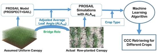
Graphical Abstract

1. Introduction

As the primary leaf photosynthesis component, chlorophyll is the most essential factor to determine the photosynthetic rate and dry matter accumulation [1,2,3]. The canopy chlorophyll content (CCC)—chlorophyll mass per unit of ground area—is the product of the leaf area index (LAI) and the leaf chlorophyll content (LCC) expressed in the unit leaf area. CCC is an important indicator reflecting the crop growth status and the canopy photosynthetic capacity [4]. The accurate acquisition of crop CCC in large-scale areas is very important for crop gross primary productivity estimation, field water and fertilizer management, pest control, and other agricultural applications [4,5,6]. However, the traditional measurements of crop chlorophyll, including the destructive laboratory method [7] and nondestructive field-portable instrument method [8], are inefficient and resource-intensive, meaning they are not applicable in large areas.
Remote sensing technology has been widely used in the retrieval of vegetation parameters because of its fast data collection and non-destructive characteristics. Due to the pigment absorption in the visible band and multiple scattering in the near-infrared band, the vegetation spectrum shows its unique characteristics in these bands, which makes it possible to use when monitoring the vegetation chlorophyll status. CCC quantifies total canopy chlorophyll content and contains both LAI and LCC information. The reflectance of red-edge bands (700–760 nm) is sensitive to chlorophyll [9] and is commonly used to retrieve the crop CCC [10,11].
Empirical, machine learning and physics-based approaches are commonly used to retrieve vegetation CCC [9,12,13]. Through statistical analysis using a vast amount of experimental data, regression relationships have been established to retrieve CCC from canopy spectra data [13,14,15]. Compared to empirical statistical models, machine learning methods have a stronger learning ability to fit complex nonlinear relationships. Machine learning methods, such as the support vector machine (SVM), artificial neural network (ANN), and random forest regression (RFR), have been widely used to retrieve vegetation parameters [16,17,18,19]. Nevertheless, training an SVM with high-dimensional data can be extremely slow [20], while ANN is prone to overfitting, and the parameter setting in ANN is more complicated [21]. Compared to SVM and ANN, RFR has proven to be a very robust machine learning algorithm for the retrieval of vegetation parameters, including the CCC [21,22]. At the same time, the retrieval models established using empirical methods or machine learning mostly use local sampled data for training. Although the empirical retrieval model is accurate for a specific type, a specific area, or a specific time period, its generalization is poor with regard to the time–space change [20]. In recent years, a new hybrid retrieval approach involving vegetation radiative transfer models (RTMs) and machine learning algorithms has been developed to compensate for limited field data [23]. The forward simulation of RTM is an important way to obtain the extensive training data needed for machine learning and is helpful for obtaining a more robust retrieval model. The PROSAIL model, a combination of the PROSPECT leaf model [24] and the arbitrary oblique leaf-scattering (SAIL) canopy model [25], is the most famous canopy reflection model. As a single-layer homogeneous canopy model, PROSAIL has been widely used for retrieving crop biochemical and structural variables [26,27,28].
RTM-based crop-CCC modeling requires attention to the interference of multiple vegetation factors, especially canopy structure factors [26,27]. At the canopy level, reflectance is not only affected by leaf biochemical parameters but is also determined by LAI, leaf inclination distribution, soil background, and other structure factors [29]. The characteristics of leaf inclination distribution—often simply the average leaf angle (ALA)—are an important canopy structure parameter that determines canopy spectral behavior. In field observation experiments and RTM simulation, ALA is an important vegetation structure parameter [30]. Although the sample size based on the SAIL forward model is large, the effects of LAI and ALA on canopy reflectance are closely related to one another, which makes it difficult to estimate LAI and ALA information accurately and simultaneously, based on the canopy spectrum [30,31]. Due to the CCC parameter containing the information of LAI, the variation in leaf inclination distribution is the main interference factor in the remote sensing retrieval of the CCC. This means it is necessary to consider prior knowledge of the ALA parameter in PROSAIL-model-based CCC retrieval for different crop types.
Introducing the prior knowledge of the ALA parameter in the PROSAIL model is a way to reduce the uncertainty of CCC retrieval across different crop types. However, there is a conflict between the homogeneous canopy assumption of SAIL and the actual crop row structure, which makes it difficult to improve the spectral simulation and retrieval of SAIL with the prior knowledge of real ALA. In addition to the ALA, the row structure also affects the proportion of exposed background soil, which is related to the reflectivity of the whole canopy [32,33]. This leads to the problem of existing differences between the measured canopy spectra and outputs of the SAIL model even when the field measurement variables are defined as the inputs of the SAIL model [34,35]. Among the simplified parameters of the PROSAIL model, ALA expresses the canopy’s geometrical properties. Therefore, the ALA input may be reasonably adjusted for the PROSAIL model in order to obtain simulated spectra that are comparable to those of the measured crop spectra [34]. It has been proven that an adjusted ALA (ALAadj) can be obtained by matching the PROSAIL model with measured spectra and non-ALA-measured parameters [34]. ALAadj for the PROSAIL model integrates leaf inclination and canopy heterogeneity information. Compared to in-situ ALA, ALAadj can better reflect the difference in canopy heterogeneity between different crop types. Therefore, prior knowledge of ALAadj has the potential to improve the performance of PROSAIL-based CCC retrieval across crop types. However, research on the application of ALAadj to vegetation parameter retrieval has not yet been carried out.
The objectives of this study were to use the ALAadj of crops as a prior knowledge input to improve the performance of RTM-based machine learning algorithms for CCC retrieval across different crop types. The mature and stable RFR algorithm was used in our work. Two important food crops, wheat and soybean, were used for algorithm testing. In this study, we evaluated the significance of ALA and other canopy parameters on crop spectra, using the PROSAIL model simulation experiment. Meanwhile, ALAadj parameterization of the PROSAIL model for wheat and soybean was carried out; then, a CCC hybrid retrieval model integrating prior ALAadj knowledge related to crop types was established. Finally, the accuracy of the improved retrieval model was evaluated using ground-measured CCC.

2. Data and Methods

2.1. Experimental Areas and Ground Data

In this study, two ground-measured datasets of wheat and soybean were used for algorithm validation and were taken from experiments carried out in Beijing, China, and Nebraska, USA, respectively. Table 1 shows the experimental locations of the collected datasets of wheat and soybean.

2.1.1. Wheat Experimental Area

The Beijing Xiaotangshan experimental area (BJ-XTS) of wheat has a temperate climate. At this site, field experiment campaigns were carried out in 2002, 2004 (detailed in [36]), and 2019. The experimental wheat plot was located at the National Station for Precision Agriculture, Xiaotangshan, Beijing, China. The biophysical parameters of winter wheat in the growing season were determined. The above wheat experiments covered erecting, early jointing, late jointing, head emergence, and filling stages. After the erecting stage, the canopy changes from open to dense as the wheat grows. In the 2002 campaign, 48 plots included four water treatment plans, four nitrogen fertilization densities, and three winter wheat varieties. In the 2004 campaign, 21 winter wheat varieties were planted with non-differentiated fertilization and irrigation management in 42 plots. In the 2019 campaign, 32 plots were analyzed, with four nitrogen fertilization densities, four fertilization treatment plans, and two winter wheat varieties.

2.1.2. Soybean Experimental Area

The experimental soybean area consisted of two AmeriFlux sites (US-Ne2 and US-Ne3), located at the University of Nebraska-Lincoln Agricultural Research and Development Center near Mead, NE, USA (https://ameriflux.lbl.gov/sites/, accessed on 28 November 2021). The US-Ne2 and US-Ne3 sites were both planted in a maize–soybean rotation model, with soybean planted in even years. The US-Ne2 site used a center-pivot irrigation system, while US-Ne3 relied entirely on rainfall for moisture. At the US-Ne2 (2002 and 2004) and US-Ne3 (2002) sites, six sub-sampling points were randomly designed to obtain spectrum and biophysical parameters (detailed in [37]).

2.1.3. Ground Data

Table 1 provides detailed information on the ground sample data.
(1)
Determination of canopy chlorophyll content
At the BJ-XTS site, fresh leaves of wheat were collected in each 1 m2 plot and then placed in a chilled box for transport to the laboratory for leaf chlorophyll content measurement (detailed in [38]). The LCC of the sampled leaves was measured by the laboratory ultraviolet-visible spectrophotometer method given in [7]. Based on the dry weight ratio of the sub-sample to the total leaf sample, the measured leaf area of the sub-sample was converted to the LAI at the BJ-XTS site. At the US-Ne2 and US-Ne3 sites, fresh leaves of soybean were collected; then, the LCC was determined through the standard procedures (detailed in [15,39]). The LAI was measured using an area meter (Model LI-3100, Li-Cor Inc., Lincoln, NE, USA). The CCC in the BJ-XTS, US-Ne2, and US-Ne3 sites were calculated by multiplying the LAI by the LCC.
(2)
Canopy reflectance measurements
The ASD FieldSpec spectrometer (Analytical Spectral Devices, Boulder, CO, USA) was used to obtain the canopy reflectance in the BJ-XTS site. The spectral range of the spectrometer was 350–2500 nm, and the spectral resolution was 3 and 10 nm in the 350–1050 and 1050–2500 nm ranges, respectively. With a standard reference plate, the canopy spectra were measured under cloudless conditions from 10 a.m. to 2 p.m. local time. The wheat canopy spectra were acquired at a field of view of 25°. In the US-Ne2 and US-Ne3 sites, the canopy reflectance spectra were measured using the Ocean Optics USB2000 radiometer (Dunedin Ocean Optics, Dunedin, FL, USA) [40]. The spectral range was 400–1100 nm, with a spectral resolution of 1.5 nm and a spectral interval of 10 nm. One radiometer measured the upward-reflected radiation of the crop canopy at a field of view of 25°. The second radiometer measured the downward solar radiation with a hemispherical field of view. The spectrum measurements were obtained under clear sky conditions from 11 a.m. to 2 p.m. local time. Then, the canopy reflectance was calculated from the measured upward and downward radiation data (detailed in [5]).
The wheat field-measured spectra were sampled in the spectral range and interval of the soybean spectral data. In order to prevent a bias, the sample size of wheat was consistent with that of 73 soybean samples, and 73 wheat samples were randomly selected from all the collected samples (shown in Table 1). The prior ALAadj knowledge of wheat and soybean was obtained by fitting the PROSAIL model using a random quarter of the measured samples. The remaining three-quarters of the measured samples were used to test the performance of our improved CCC retrieval algorithm.

2.2. Spectra Simulation

2.2.1. Spectra Simulation of Homogeneous Canopy Based on PROSAIL Model

As an improved version of the PROSAIL model, the PROSAIL-D model, coupled with the PROSPECT-D leaf model [41] and the 4SAIL canopy model [42], was used to simulate crop canopy spectrum in the 400–2500 nm wavelength range for training the CCC retrieval model, with the input parameter settings as in Table 2.
In the leaf parameters of the PROSPECT-D model, the LCC value was set between 10 and 80 μg cm−2. Carotene accounts for 25% of the content of the LCC and changes with the LCC. The leaf dry matter content (Cm) ranged from 0.003 to 0.006 g cm−2, and the setting range of the leaf structure parameter (N) was 1.0~2.0. Equivalent water thickness was set to a fixed value because the water absorption bands are generally not used in the retrieval of vegetation chlorophyll.
The canopy structure in the 4SAIL model was defined by the LAI, ALA, soil reflectance, and hot-spot parameters (shown in Table 2). The LAI value was set between 0.5 and 8. Two widely used modes of leaf inclination angle distribution function (LIDF), including Campbell’s algorithm [43] and Verhoef’s algorithm [44], have been implemented in multiple versions of SAIL codes. Horizontal leaves can have higher light interception capabilities, and a certain number of horizontal leaves is a common state in canopy plants [45]. The ellipsoid function in Campbell’s algorithm causes the probability density of zero when the leaf angle is zero or close to zero, which is inconsistent with the actual canopy situation [46]. Verhoef’s leaf inclination distribution algorithm, using a linear combination of trigonometric functions, improves this problem [44]. Therefore, Verhoef’s algorithm with the LIDF parameters was selected for the PROSAIL-D simulation in this study. LIDFa and LIDFb control the ALA and the distribution bimodality, respectively. The ALA values in degrees calculated from LIDFa can be expressed as ALA = 45–360 × LIDFa/π2 [44], ranging from 10 to 80 degrees. Compared to ALA, LIDFb has a very small effect on canopy reflectance [29], and the setting of LIDFb was fixed at 0. To represent the soil background variations, the measured spectra of bare and dry soil were multiplied by the brightness coefficients of five gradients (0.1, 0.25, 0.5, 0.75, and 1), and five soil spectra from light to dark were determined for the PROSAIL-D simulation. According to the field sampling of the canopy spectrum at nadir, a fixed observation zenith angle of 0 degrees and the variable sun angle values were set.

2.2.2. Spectra Simulation of the Heterogeneous Canopy with Mixed Pixels

The SAIL model as a part of the PROSAIL model is a turbid medium model that expresses a homogeneous canopy. The SAIL model assumes that the canopy is composed of extremely small leaves randomly distributed in the horizontal layer [25]. However, the assumption of homogeneous canopy conditions in the PROSAIL model is inconsistent with the actual heterogeneity of most row-sown crops. Different crops have different leaf inclination characteristics, and their planting structures also have large discrepancies. For example, a canopy of row-planted crops has more soil exposed than a uniform canopy [33,35]. Taking mixed pixels as a special case of a heterogeneous canopy, the influence of the canopy heterogeneity factor on reflectance was evaluated in this study.
The spectral linear mixing method [47] was used to fit the reflectance of vegetation-soil mixed pixels, named Rmixed:
R mixed = R veg × ( 1 FC soil ) +   R soil ×   FC soil
where Rveg is the reflectance of the pure vegetation-covered endmember based on PROSAIL simulations, Rsoil is the reflectance of the soil endmember, FCsoil is a fractional cover of the soil endmember, and the range of FCsoil was set from 0% to 50%.

2.3. Methods

The specific flow chart of the method is shown in Figure 1.

2.3.1. Random Forest

As an advanced machine learning algorithm, random forest is considered to demonstrate accurate prediction and good fault tolerance [48,49]. We used random forest for evaluating the influence of ALA and other vegetation parameters on reflectance, as well as adjusting the ALA for the PROSAIL model, based on measured spectrum and non-ALA parameters and retrieving CCC by involving the crop-type-related ALAadj. Random forest uses many decision trees to train samples and make predictions. A decision tree is a statistical model of supervised classification that is constructed through the training set for prediction or classification. Random forest is an improvement of multiple decision trees, based on the bagging strategy [50]. After selecting samples, k attributes are randomly selected from the sample attributes, and then the information gain and Gini index methods are used to continuously find the best-separated attributes to establish a cart decision tree. The above process is repeated to establish m classifiers; these decision trees can then be used to form a random forest, and prediction results can be obtained via averaging.
In fact, random forest is a common method in the field of machine learning, which can be used for the nonlinear regression of a large amount of data and retrieval of vegetation parameters, using a radiative transfer model such as PROSAIL. The random forest method has the following characteristics [51,52]: (1) in the current machine learning algorithms, it has a fairly high accuracy; (2) it can run effectively on huge datasets; (3) it is able to process input data with high-dimensional features; (4) it can evaluate the importance of each variable; (5) it can obtain unbiased estimates of internally generated errors; (6) it can also give good results for the discrete values of inputs. By using MATLAB software (The Math Works, Natick, MA, USA) in this study, the simulation dataset was divided into 100 homogeneous subsets, that is, the results of establishing 100 trees were averaged to achieve the final prediction.

2.3.2. Importance Assessment Method of Vegetation Variables on Canopy Reflectance

The variable importance measures of RFR were used to evaluate the contribution of different vegetation parameters to reflectance at the visible and near-infrared (NIR) wavelengths before 900 nm. Random forest is a Bayesian prediction of the decision tree, which can provide a flexible mapping relationship between input and output and provide a measure of the importance of variables. In addition to the importance evaluation of the quantitative input–output relationship, global importance evaluation can be carried out for situations where the input or output variables are not quantifiable, such as soil types. Field-measured data have some inherent natural limitations; for example, there is usually a certain autocorrelation between the LCC and LAI, which is not conducive to the global importance analysis of ALA on reflectance. Each parameter in the simulation data can be set to be completely independent, based on the physical model such as PROSAIL, so it is suitable to carry out an impact contribution evaluation of vegetation variables on vegetation reflectance [34,53].
In this study, the random forest algorithm is used to train the nonlinear relationship between parameters and reflectivity at different wavelengths, and to simultaneously calculate the importance of all independent variables versus dependent variables. Leaf and canopy parameters, including the LCC, N, Cm, LAI, Rsoil, ALA, and FCsoil, are the independent variables, while the PROSAIL-simulated reflectance for the homogeneous canopy case and the mixed pixels cases act as the dependent variable.

2.3.3. PROSAIL Parameterization Scheme of ALAadj Based on Measured Spectrum and Non-ALA Parameters

The same LAI corresponds to a larger soil fraction under a spatially heterogeneous canopy than that under a homogeneous canopy [54]. ALA variation changes the gap of the homogeneous canopy in a specific observation direction [25,54,55], which leads to the ALAadj being used to make the PROSAIL model suitable for the use of spatially heterogeneous canopy cases. The conceptual diagram in Figure 2 describes the role of ALAadj in improving the applicability of the PROSAIL model on a homogeneous canopy. In Figure 2a, we simplified the homogeneous canopy as a leaf completely covering the ground, and the leaf angle is ALA. For the special case shown in Figure 2a, the corresponding ground area covered by the leaf is calculated based on ALA, as below:
LA * cos ( ALA ) = A
where A is the ground area; LA is the leaf area, here, LAI = LA/A. Figure 2b shows that, in the case of a mixed pixel canopy with the same LAI, the leaf clumping effect causes a gap fraction of the soil endmember. The gap fraction of the soil endmember is a. In fact, a/A is equivalent to FCsoil, the ratio of soil endmember in a mixed vegetation-soil pixel. The limitation of the PROSAIL model to simulate heterogeneous canopy reflectance may affect the performance of a PROSAIL-based hybrid model of CCC retrieval. Figure 2c shows that the homogeneous canopy case with the leaf angle adjusted to ALAadj has the same gap fraction as the heterogeneous canopy case in Figure 2b. The ground area, calculated based on ALAadj in Figure 2c, can be determined as below:
LA *   cos ( ALA adj ) + a = A
where a is the same soil gap as that in Figure 2b. Figure 2c shows that the ALAadj can compensate for the increase in soil gap caused by the leaf aggregation effect at a specific observation direction, which may make the PROSAIL-simulated spectrum more consistent with that of an actual row-planted canopy.
Through fitting the PROSAIL simulations with the measured spectrum, and non-ALA parameters such as LAI, the ALA can be adjusted [34]; that is, the prior ALAadj knowledge for wheat and soybean can be obtained. The prior ALAadj knowledge for one crop type is simply characterized by the average ALAadj. Inversion of the PROSAIL model generally obtains the fitted parameters to match the measured data through three ways: the iterative optimization, based on the forward programming of the physical model, the look-up table (LUT), and the machine learning method. Compared to the program loop call, LUT improves the calculation speed and avoids the risk of converging to local minima [56], while the machine learning approach saves abundant storage space compared to the LUT approach [32].
In this study, the RFR was used for optimizing the ALA of the PROSAIL model based on ground-measured data; then, the ALAadj of wheat and soybean was obtained. Optimizing ALA requires determining the measured vegetation parameters and the used bands. Due to the overlap of response areas of the LAI and ALA, as well as the CCC containing LAI information, ALA optimization for the PROSAIL model needs the measured LAI data, in addition to the spectrum. LCC was used as supplementary measured data (Figures S1 and S2). In the case of additional data, it also participated in the PROSAIL model fitting process to obtain ALAadj. Based on the analysis of the measured and simulated data, it was found that the main spectral response regions of ALA are the red-edge and near-infrared regions [34,57]. We considered the sensitive response bands of canopy ALA to optimize ALA when using measured spectra and non-ALA vegetation parameters. The specific ALAadj formula, based on RFR, is as follows:
ALA adj = RFR   ( SPEC ,   LAI measured ,   LCC measured )
where SPEC is the canopy reflectance, and LAImeasured and LCCmeasured are the ground-measured LAI and LCC values. Considering the presence or absence of chlorophyll, there are two combinations of inputs: (a) SPEC_LAI, meaning that the input data have reflectance and are LAImeasured; (b) SPEC_LAI_LCC, meaning the input data have reflectance and are LAImeasured and LCCmeasured.

2.3.4. CCC Retrieval Model, Based on ALAadj Related to Crop Types

In this study, the PROSAIL-D model was used to simulate the canopy’s spectral reflectance, and a training dataset containing multiple parameter variations, such as ALA, LAI, and LCC was established. The CCC retrieval RFR models were established, whether prior ALAadj knowledge was used or not. We used RFR to identify the bands related to vegetation biochemical characteristics in different spectral datasets. RFR randomly selected the feature number for each decision tree and determined the best feature number. Its hyperparameters mainly included the number of growing decision trees. Too few trees result in weak learning ability, so the number of trees was set to 100.
In order to compare and analyze the influence of the different ALAadj of wheat and soybean on the retrieval model, two kinds of algorithms considering the prior ALAadj knowledge, related to crop types or not, were designed and tested. First, the algorithm advocated in this study was used to select the corresponding ALAadj-based RFR model to carry out CCC retrieval for wheat and soybean, named the Prior-ALA model. Second, we designed three NonPrior-ALA models for the CCC retrieval of soybean and wheat, without considering the prior ALA knowledge corresponding to the differences in vegetation types. The three NonPrior-ALA models included: (a) model training only using PROSAIL-simulated data with the wheat ALAadj; (b) model training with the soybean ALAadj; (c) model training with both wheat and soybean ALAadj.
Due to the difference in the number of sampling bands of different remote sensors, the impact of band number on canopy chlorophyll machine learning was investigated and evaluated. The continuous spectrum data and the different numbers of discrete band data were used to test the CCC retrieval model. The continuous spectrum adopted the 50 narrow-band ground spectra within 400–890 nm that are related to chlorophyll, and the discrete bands referred to the settings of Envisat MERIS and Sentinel-3 OLCI bands. MERIS and OLCI are two important satellite sensors with red-edge bands and have very overlapping band settings (Table 3). Referring to MERIS reflectance products, we selected all available bands (13 bands) after removing the three main atmospheric bands (aerosol: B1; oxygen: B11; water vapor: B15). The blue band is susceptible to residual aerosol effects [58], so we also selected fewer bands (nine bands) after removing the bands adjacent to blue. As given in Table 3, the three combinations of independent variables for the CCC estimation were: (1) all continuous reflectance (50 bands) within 400–890 nm; (2) the reflectance of all available bands in MERIS (13 bands): B1, B2, B3, B4, B5, B6, B7, B8, B9, B10, B12, B13, and B14; (3) nine selected MERIS bands (nine bands) from the green to near-infrared regions: B5, B6, B7, B8, B9, B10, B12, B13, and B14. The simulated spectra were resampled using the MERIS spectral function to obtain 13- and 9-band datasets.

2.3.5. Validation Method

Using ground reflectance data, CCC retrieval for wheat and soybean was carried out, and the accuracy of this CCC inversion was verified by ground validation data. When evaluating the accuracy of CCC retrieval, we should consider not only the determination coefficient (R2) for the estimation results and ground-based validation data but also the root mean square error (RMSE) and bias (Bias). The formulas for R2, RMSE, and Bias are as follows:
R 2 = i n ( y ^ i   y ¯ ) i n ( y i   y ¯ ) RMSE = i = 1 n ( y ^ i y i ) 2 n Bias = i n ( y i y ^ i ) n
where y ^ i represents the estimated CCC value, yi represents the measured CCC value, y ¯ represents the mean of estimated CCC values, and n represents the number of test samples.

3. Results and Analysis

3.1. Influences of Vegetation Variables on Canopy Reflectance

Figure 3 shows the estimation results of the importance of multiple vegetation factors for visible and NIR reflectance, based on random forest regression analysis, in the case of both a homogeneous canopy and a heterogeneous canopy with mixed pixels.
For the first case in which the PROSAIL model simulated the reflectance of a uniform canopy, LCC, LAI and ALA contributed significantly to the tested bands before 900 nm. Of the three most important factors, the LCC and LAI are the composition parameters of the CCC. The LCC has the highest contribution importance on the canopy reflectance, especially before 710 nm. The N value has a certain influence on the 560 nm and 710 nm bands, but less influence on the other bands. There is little influence of Cm on all the visible and NIR bands that were tested. Among the canopy parameters, the LAI is still the most important driving factor affecting canopy reflectance, followed by the ALA. The importance of soil reflectance changes is equivalent to the ALA in the 490 nm and 680 nm bands and is far lower than that of the LAI and ALA in other bands. The global sensitivity analysis results of the PROSAIL model reported in [29,34] showed that the LCC had a leading role before 710 nm and that LAI and ALA were the two main driving forces for the reflectance change, which is basically consistent with our variable importance measures results for the homogeneous canopy scenario. This shows that the variable importance analysis method of using random forest to evaluate the multi-factor contributions of canopy reflectance is also reliable.
In the case of vegetation–soil mixed pixels, which is a special non-uniform canopy scenario, the importance values of LCC and other leaf parameters to the tested bands are similar to the result for the uniform canopy scenario. However, an obvious difference is that FCsoil has become a new influencing factor of canopy reflectance, and its influence in the 750 nm and 860 nm bands is greater than the ALA but only less than the LAI. In addition, the mixed pixel effect greatly enhances the influence of the ALA and Rsoil on visible and NIR reflectance. It is worth noting that the Rsoil has a greater impact on low vegetation reflectance in the visible bands than the ALA while having a lower impact on the red-edge and NIR bands. The results of the RFR importance analysis of the mixed-pixel scenario show that the spectral contribution of the LAI was easily confused, not only with the ALA factor but also with FCsoil. Therefore, the sensitivity of canopy reflectance to the ALA and other heterogeneous canopy factors, such as FCsoil, should be considered in CCC retrieval for crops that are usually planted in rows.

3.2. ALAadj Parameterization of the PROSAIL Model for Wheat and Soybean

An ALA optimization model was established by the random forest algorithm, based on PROSAIL-simulated data (Section 2.2). As seen in Figure 3, the reflectance of the 710–890 nm bands was selected for ALA optimization. Table 4 shows that the average values of wheat ALAadj obtained by PROSAIL optimization, based on the canopy spectra and the measured LAI with or without LCC, were very close (62.0 and 61.8 degrees respectively), and the prior knowledge of wheat ALAadj for this study was set to 62 degrees. The soybean ALAadj obtained from the two sets of data was 45.1 and 45.7 degrees, respectively. In this study, the prior knowledge of soybean ALAadj was set to 45 degrees. Whether or not LCC was involved, the results of ALAadj for wheat and soybean were stable, and there was a clear distinction between the ALAadj of wheat and soybean.

3.3. CCC Retrieval with Prior ALAadj Knowledge for Wheat and Soybean

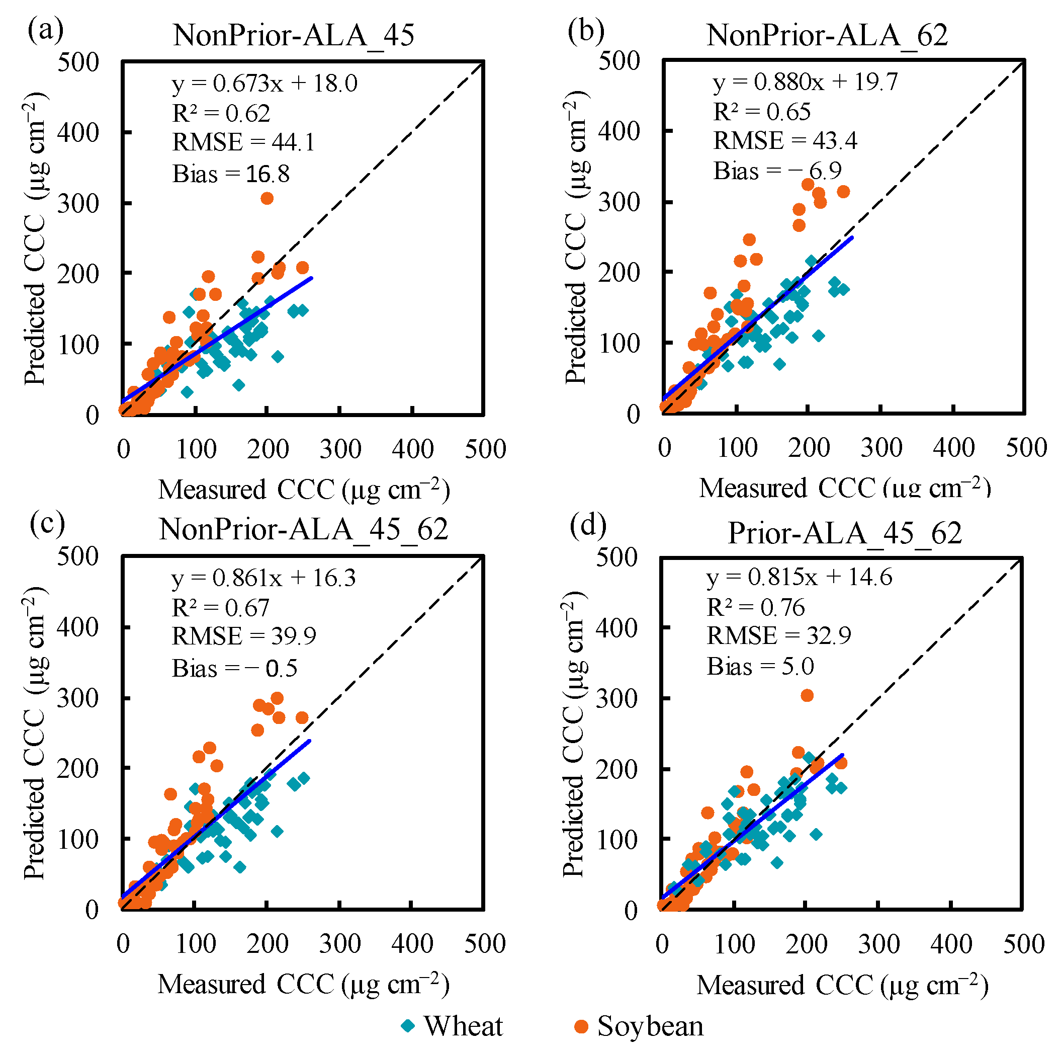
Figure 4 provides the validation of CCC retrieval based on the ground-measured continuous spectra, considering prior ALAadj knowledge or not. Figure 4a shows that the NonPrior-ALA_45 model constructed by PROSAIL simulations, with an ALAadj of 45 degrees, had a good correlation between the estimated and measured CCC values of soybean but the CCC value of wheat was underestimated, especially when the CCC was relatively large. Figure 4b shows that the NonPrior-ALA_62 model produced a very good CCC estimation of wheat but produced an overestimation of the soybean CCC. Figure 4c shows that the NonPrior-ALA_45_62 model underestimated the CCC for wheat and overestimated the CCC for soybean. Compared to the three models without considering prior ALA, the test results of the random forest model with a prior (Prior-ALA_45_62) (Figure 4d) showed no obvious overestimation of wheat or soybean, and its retrieval accuracy (R2 = 0.76, RMSE = 32.9 μg cm−2) was better than all three CCC models without prior ALAadj knowledge related to crop types (NonPrior-ALA_45: R2 = 0.62, RMSE = 44.1 μg cm−2; NonPrior-ALA_62: R2 = 0.65, RMSE = 43.4 μg cm−2; NonPrior-ALA_45_62: R2 = 0.67, RMSE = 39.9 μg cm−2).
Table 5 shows the performance differences of the CCC retrieval models for wheat and soybean. In the validation results for wheat samples, it was found that the NonPrior-ALA_62 model, trained by the PROSAIL-simulated data with our proposed wheat ALAadj (62 degrees), showed higher CCC retrieval accuracy (RMSE = 37.9 μg cm−2) than the other two models (NonPrior-ALA_45: RMSE = 56.2 μg cm−2; NonPrior-ALA_45_62: RMSE = 39.4 μg cm−2). In the validation results for the soybean samples, the CCC accuracy (RMSE = 26.9 μg cm−2) of the NonPrior-ALA_45 model corresponding to the proposed soybean ALAadj (45 degrees) was better than the other two (NonPrior-ALA_62: RMSE = 48.2 μg cm−2; NonPrior-ALA_45_62: RMSE = 40.3 μg cm−2). The difference in the wheat or soybean CCC RMSE values for the above three models was large, which was not only caused mainly by the change in R2 but also by the large variation of Bias. This shows that when the ALA of the PROSAIL simulations did not match the prior ALAadj knowledge corresponding to the test crop, the RFR algorithm produced a larger CCC retrieval error. For comprehensive test samples of the two crops, the Prior-ALA_45_62 model that considered prior knowledge of crop type-related ALAadj obtained the best performance.

3.4. Performance Comparison of the Improved CCC Retrieval Model Using Continuous and Discrete Spectra

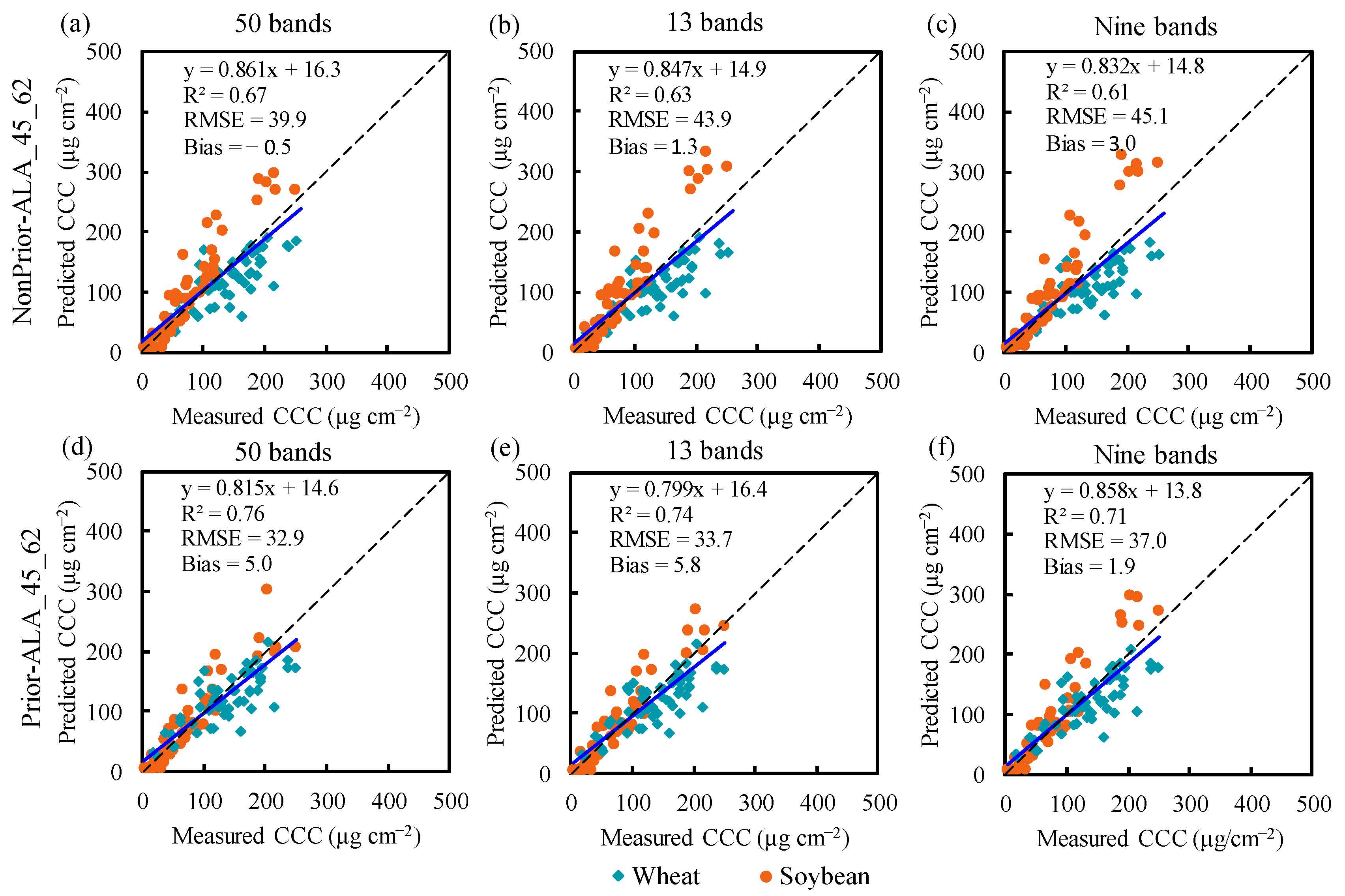
Figure 5 shows the validation and comparison results of the CCC retrieval models using the continuous and discrete bands. In the case of not considering the prior knowledge of crop-type-related ALAadj, using the reflectance of the continuous waveband can obtain the highest CCC retrieval accuracy (Figure 5a). As the resolution decreased, the accuracy of CCC retrieval was slightly reduced (Figure 5b,c). In the scenario where the prior ALAadj knowledge is included, the accuracy had a similar relationship with the number of input bands (Figure 5d–f). Figure 5 also indicates that, after considering the prior ALAadj knowledge, the CCC retrieval accuracy using the continuous and discrete spectra significantly increased. The RMSE of the improved CCC retrieval model using the 50-band continuous reflectance decreased by 7.0 μg cm−2 and the R2 increased by 0.09; the RMSE of the improved model using the 13-band discrete reflectance decreased by 10.2 μg cm−2 and the R2 increased by 0.11; the RMSE of the improved model, using the nine-band discrete reflectance, reduced by 8.1 μg cm−2 and the R2 increased by 0.10. Using any of the three different band combinations, the accuracy of the improved CCC retrieval models (RMSE: 32.9~37.0 μg cm−2; R2: 0.71~0.76) was higher than those of models not involving crop-type-related ALAadj parameterization (RMSE: 39.9~45.1 μg cm−2; R2: 0.61~0.67). In other words, the influence of crop-type-related ALAadj parameterization on CCC retrieval is larger than that of the difference among the three band selections in this study.

4. Discussion

4.1. Contribution of Our Proposed Method to PROSAIL-Based Retrieval of Crop Parameters

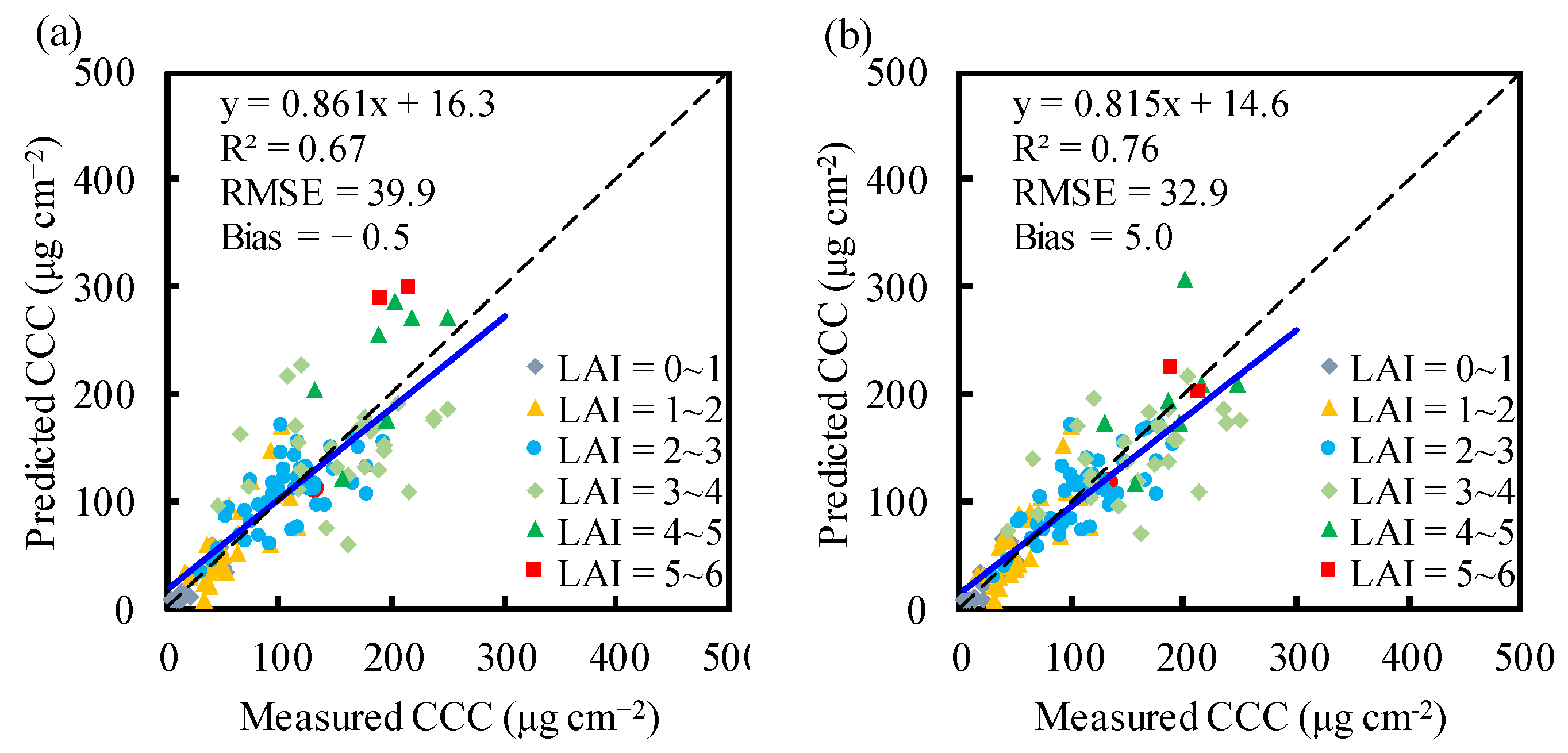
This study proposed an ALAadj parameterization scheme to improve the performance of the PROSAIL model in the CCC estimation for different crops. The PROSAIL model simplifies the scene and parameters, making it straightforward and easy to use, but the non-uniform canopy assumptions of the PROSAIL model also limit the application of the PROSAIL model for a non-uniform canopy. For example, the PROSAIL-simulated spectrum using measured vegetation parameters is inconsistent with the simultaneously measured spectra [34]. This problem limits the vegetation parameter hybrid retrieval based on the PROSAIL simulations, as shown in Section 3.3 and Section 3.4 of this paper. Establishing model parameterization schemes according to actual scenes or research objects is an important way to improve the simulation accuracy of vegetation RTMs [19,59,60]. For the PROSAIL model, the ALA is considered to be the structural parameter that has the greatest impact on reflectance, besides the LAI [31,61]. The LAI quantifying the number of leaves cannot be used to express the degree of canopy spatial heterogeneity, while the ALAadj can achieve a different canopy gap fraction under the same LAI (shown in Figure 2) and make the PROSAIL simulations adapt to a heterogeneous canopy. It has been proven that PROSAIL simulations with ALAadj can maintain better consistency with the measured spectra of wheat and maize [34]. Due to the conflict between PROSAIL simulations and the actual canopy spectra of row-planted crops, error of the crop CCC estimates occurs when appropriate ALAadj parameterization is not considered in the PROSAIL-based hybrid model of CCC retrieval; in particular, the CCC estimation error in medium and high LAI samples is obvious (Figure 6a). In this study, the RFR algorithm of CCC estimation with ALAadj parameterization drastically alleviated the problem of substantial error in medium and high LAI crop samples (Figure 6b).
In the previous studies on RTM-based CCC retrieval, Xing [62] reported their best result for wheat CCC estimates obtained from PROSAIL-based regression models using VIs (wheat: RMSE = 104.66 μg cm−2), which is worse than the result (shown in Table 5) of using our unimproved RFR model (wheat: RMSE = 39.4 μg cm−2) or improved RFR model (wheat: RMSE = 37.9 μg cm−2). This indicates that the advantages of advanced machine learning algorithms such as RFR in non-linear learning may play a role. Sun [63] used a PROSAIL-based RFR model with two VIS inputs (MTCI and MTVI2) to obtain a comprehensive wheat and soybean result of CCC retrieval with an RMSE of 37.76 μg cm−2, which is similar to that from our unimproved RFR model using reflectance spectra (wheat and soybean: RMSE = 39.9 μg cm−2) but is worse than that when using our improved RFR model (wheat and soybean: RMSE = 32.9 μg cm−2). In addition, the accuracy of soybean CCC estimates from our improved physical-based model (soybean: RMSE = 26.9 μg cm−2) is not as good as the best accuracy of soybean CCC estimates from the locally calibrated empirical model using CIred-edge (soybean: RMSE = 16 μg cm−2) reported by Clevers [64]. This may be understandable because hybrid algorithms based on RTMs have strong generalization abilities and empirical models using local calibration have advantages in local areas [32]. To the best of our knowledge, this is the first time that prior information of crop type-related ALAadj has been involved in the PROSAIL-based retrieval of vegetation parameters. This study provides a new design idea for RTM-based machine learning algorithms for retrieving other parameters across different crop types.
This study used a special heterogeneous canopy scenario—an ideal mixture of vegetation and soil—to show that the canopy spatial heterogeneity of row crops can have a great impact on the spectral reflectance, related to CCC. There are other characteristics of crop canopy structure that are not considered by the PROSAIL model, such as leaf and stem morphology [65,66]. They may cause spectral differences between different crops under the same CCC and affect the performance of a PROSAIL-based CCC retrieval model. There are great differences in these canopy characteristics between crop types, which makes cross-crop-type CCC retrieval rather difficult. This study aimed to address this problem, and improved CCC retrieval for wheat and soybean by introducing ALAadj parameterization into a PROSAIL-based RFR algorithm. In addition, the growth dynamics of crops within the same type are accompanied by changes in the attributes of these canopy structure factors [66]. Our wheat case (shown in Figure S2) shows that variations in growth stages increased the difficulty of CCC modeling even for the same crop, although our proposed method improved the accuracy of wheat CCC retrieval (especially in terms of Bias). Based on more crop structure measurements and advanced 3D canopy models, it will be very valuable to carry out quantitative analysis of the impact of LAI, ALA, leaf morphology, stem composition, and other canopy heterogeneity factors on the CCC retrieval of cross-type crops in the future.

4.2. Reliability and Limitation of the ALAadj Parameterization Associated with Crop Types

A feasible scheme of ALAadj parameterization for the PROSAIL model is crucial to improving the hybrid machine learning algorithms for CCC estimation. In addition to the spectral data, the LAI provides the necessary measured data for an ALAadj parameterization scheme. This is because the LAI and ALA have overlapping effects on reflectance, and they are difficult to separate by spectral retrieval [19]. Our research found that ALAadj calculation based on the measured LAI and canopy spectrum can obtain stable results, regardless of whether chlorophyll is involved or not (as shown in Table 4). In addition, LAI samples are easier to obtain than LCC samples in the field. Consequently, the use of the canopy spectrum and measured LAI is also a practical and feasible ALAadj parameterization scheme.
ALAadj containing canopy ALA information, as well as other canopy structure information, has the ability to reflect the differences in canopy structure for different crops, which was proven in our parameterized ALAadj results, showing obvious differences between wheat and soybean. Our ALAadj parameterization results of the wheat sample (ALAadj = 62 degrees) was similar to the wheat results (ALAadj = 60.5 degrees) reported in the literature [34]. The wheat ALA values were reported to be generally greater than the soybean ALA [34,53,67], which is similar to our own ALAadj comparison results between wheat and soybean. However, the correlation between ALAadj and ALA was found to not be very strong [34], which shows that ALAadj not only contains ALA information but also canopy structure information other than LAI and ALA. The plant types of different crops are obviously variable, and the planting structures of the same crops are similar. That results in more consistent ALAadj within the crop types, and larger differences in inter-type ALAadj values, although ALA may vary with different growth stages or different varieties for a given crop type [57,61]. Therefore, ALAadj related to crop types can become an effective prior knowledge that can be used in CCC retrieval models across different crop types.
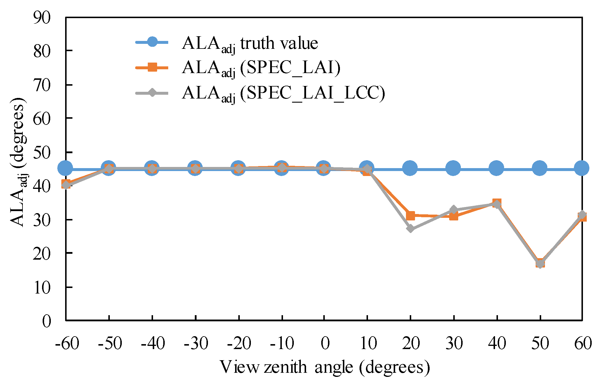
The obtained ALAadj for nadir observation in this study may be not suitable for all observation angles. By using our ALAadj parameterization model for nadir observation and PROSAIL-simulated data with a fixed ALA of 45 degrees, the influence of different view zenith angles (VZAs) on the ALAadj parameterization was shown in Figure 7. The PROSAIL-simulated spectra correspond to a homogeneous canopy; the ALA input of 45 degrees should be the true ALAadj value in this case. The obtained ALAadj values close to the nadir are more accurate than those far from the nadir, which implies that the extraction and application of prior ALAadj knowledge must consider the VZA matching. To solve the problem of ALAadj application with large-angle observation, one possible approach is to generate a prior knowledge matrix of ALAadj related to both crop types and VZAs.
Verhoef’s leaf inclination distribution mode was used for ALA optimization in this study. In addition, there are other leaf inclination distribution modes that have a certain influence on canopy spectra simulation [55]. Therefore, the leaf inclination distribution modes used in the acquisition and application of crop-type-related ALAadj with the PROSAIL model need to be the same. This study only tested the cases of wheat and soybean. In future investigations, for more crops with a complex canopy structure, it is necessary to carry out new and more precise tests of ALAadj parameterization for the PROSAIL model.

4.3. Prospects of Our Proposed Method of Crop CCC Estimation Based on Satellite Data

With the exception of prior ALAadj knowledge of different types, the satellite-scale CCC retrieval also requires the spatial distribution of crop types to determine the ALAadj value. The development of vegetation-type mapping products is becoming increasingly better [68,69,70], and the promotion of the hybrid vegetation retrieval model with ALAadj parameterization has a chance of receiving better support.
In this study, the improved method was based on the ground reflectance spectrum. In addition to continuous reflectance (50 bands), we also tested discrete band combinations (13 and nine bands) with reference to MERIS and Sentinel satellite data. It was found that the performance of the discrete spectrum was worse than that of the continuous spectrum, which is similar to other parameterization studies [71,72]. The small reduction is also acceptable in the discrete band (Figure 5), which shows that the method has the potential to be extended to discrete satellite remote-sensing data.
In addition, there are some uncertainties in the actual satellite data, including remote sensor hardware indicators, atmospheric correction processing [73], and complex ground mixing [74]. Future research can try to use Sentinel-2, Sentinel-3, and other satellites to estimate and test the canopy chlorophyll content of satellite-to-ground synchronization, to further verify the applicability of the proposed algorithm on the satellite scale.

5. Conclusions

In this study, through the evaluation of the variable importance of canopy reflectance based on the random forest algorithm, it was found that the PROSAIL model had difficulty in expressing a spatially heterogeneous canopy with vegetation–soil mixed effects caused by crop-row planting. Given that the ALA input of the PROSAIL model is related to the gap of the canopy, ALA adjustment based on measured spectra and non-ALA parameters can take into account the influence of the ALA and canopy spatial heterogeneity on the crop reflectance in a specific observation direction. In view of the limitations of the PROSAIL model in expressing the complexity of vegetation structure, this study proposed an RFR algorithm of crop CCC retrieval that is trained with PROSAIL simulations, with prior ALAadj knowledge. The applicability of the algorithm was tested using measured wheat and soybean data. The results show that the parameterized values of ALAadj (62 degrees for wheat; 45 degrees for soybean), fitted based on ground-measured data, showed good discrimination between the two crop types. The CCC retrieval accuracy (RMSE from 39.9 to 32.9 μg cm−2; R2 from 0.67 to 0.76) of wheat and soybean ground continuous spectra (50 bands) was improved by integrating the prior knowledge of wheat and soybean ALAadj parameterization. In addition, this method also performed well under discrete reflectance data (13 bands: RMSE from 43.9 to 33.7 μg cm−2; R2 from 0.63 to 0.74; nine bands: RMSE from 45.1 to 37.0 μg cm−2; R2 from 0.61 to 0.71). The findings reveal that the ALAadj parameterization for the PROSAIL model helps to improve the performance of RFR hybrid algorithms of CCC retrieval across crop types. With the support of crop type (survey or satellite) products, our proposed CCC retrieval algorithm involving ALAadj parameterization related to crop types will offer the beneficial potential of application on a large scale, as well as providing a good reference for an RTM-based hybrid algorithm for other crop parameter estimations.

Supplementary Materials

The following supporting information can be downloaded at: https://www.mdpi.com/article/10.3390/rs14010098/s1, Figure S1: Five soil spectra from light to dark used in the PROSAIL simulations, Figure S2: Accuracy of CCC retrieval characterized by different growth stages for wheat using ground-measured continuous spectra (a) without and (b) with considering prior ALAadj knowledge related to crop types.

Author Contributions

Conceptualization: Q.J. and B.Z.; methodology: Q.J., W.H. and B.Z.; validation: Q.J. and Q.S.; formal analysis: Q.S. and Q.J.; investigation: Q.J.; data curation: Q.J., Q.S., H.Y. and B.Q.; writing—original draft preparation: Q.J.; writing—review and editing: H.Y. and Z.Z.; visualization: Q.J. and Q.S.; supervision: W.H. and X.Z. All authors have read and agreed to the published version of the manuscript.

Funding

This research was funded by the National Natural Science Foundation of China (grant number 42030111 and 42071330) and the Youth Innovation Promotion Association CAS (grant number 2021119).

Institutional Review Board Statement

Not applicable.

Informed Consent Statement

Not applicable.

Acknowledgments

We appreciate the soybean data provided by the Center for Advanced Land Management Information Technologies (CALMIT), University of Nebraska–Lincoln. We also appreciate to the experimenters who participated in wheat experiments in Beijing Xiaotangshan Site.

Conflicts of Interest

The authors declare no conflict of interest.

References

  1. Ustin, S.L.; Gitelson, A.A.; Jacquemoud, S.; Schaepman, M.; Asner, G.P.; Gamon, J.A.; Zarco-Tejada, P.J. Retrieval of foliar information about plant pigment systems from high resolution spectroscopy. Remote Sens. Environ. 2019, 113, S67–S77. [Google Scholar] [CrossRef] [Green Version]
  2. Croft, H.; Chen, J.M.; Zhang, Y. The applicability of empirical vegetation indices for determining leaf chlorophyll content over different leaf and canopy structures. Ecol. Complex. 2014, 17, 119–130. [Google Scholar] [CrossRef]
  3. Croft, H.; Chen, J.M.; Luo, X.; Bartlett, P.; Chen, B.; Staebler, R.M. Leaf chlorophyll content as a proxy for leaf photosynthetic capacity. Glob. Chang. Biol. 2017, 23, 3513–3524. [Google Scholar] [CrossRef]
  4. He, R.; Li, H.; Qiao, X.; Jiang, J. Using wavelet analysis of hyperspectral remote-sensing data to estimate canopy chlorophyll content of winter wheat under stripe rust stress. Int. J. Remote Sens. 2018, 39, 4059–4076. [Google Scholar] [CrossRef]
  5. Gitelson, A.A.; Viña, A.; Verma, S.B.; Rundquist, D.C.; Arkebauer, T.J.; Keydan, G.; Leavitt, B.; Ciganda, V.; Burba, G.G.; Suyker, A.E. Relationship between gross primary production and chlorophyll content in crops: Implications for the synoptic monitoring of vegetation productivity. J. Geophys. Res. Atmos. 2006, 111. [Google Scholar] [CrossRef] [Green Version]
  6. Gitelson, A.A.; Peng, Y.; Arkebauer, T.J.; Schepers, J. Relationships between gross primary production, green LAI, and canopy chlorophyll content in maize: Implications for remote sensing of primary production. Remote Sens. Environ. 2014, 144, 65–72. [Google Scholar] [CrossRef]
  7. Porra, R.J. The chequered history of the development and use of simultaneous equations for the accurate determination of chlorophylls a and b. Photosynth. Res. 2002, 73, 149–156. [Google Scholar] [CrossRef]
  8. Cerovic, Z.G.; Masdoumier, G.; Ghozlen, N.B.; Latouche, G. A new optical leaf-clip meter for simultaneous non-destructive assessment of leaf chlorophyll and epidermal flavonoids. Physiol. Plant. 2012, 146, 251–260. [Google Scholar] [CrossRef]
  9. Pinar, A.; Curran, P.J. Grass chlorophyll and the reflflectance red edge. Int. J. Remote Sens. 1996, 17, 351–357. [Google Scholar] [CrossRef]
  10. Maccioni, A.; Agati, G.; Mazzinghi, P. New vegetation indices for remote measurement of chlorophylls based on leaf directional reflectance spectra. J. Photochem. Photobiol. B Biol. 2001, 61, 52–61. [Google Scholar] [CrossRef]
  11. Gitelson, A.A.; Gritz, Y.; Merzlyak, M.N. Relationships between leaf chlorophyll content and spectral reflectance and algorithms for non-destructive chlorophyll assessment in higher plant leaves. J. Plant. Physiol. 2003, 160, 271–282. [Google Scholar] [CrossRef]
  12. Cui, S.; Zhou, K. A comparison of the predictive potential of various vegetation indices for leaf chlorophyll content. Earth Sci. Inform. 2017, 10, 169–181. [Google Scholar] [CrossRef]
  13. Peng, Y.; Anthony, N.R.; Timothy, A.; Gitelson, A.A. Assessment of canopy chlorophyll content retrieval in maize and soybean: Implications of hysteresis on the development of generic algorithms. Remote Sens. 2017, 9, 226. [Google Scholar] [CrossRef] [Green Version]
  14. Dash, J.; Curran, P.J. The MERIS terrestrial chlorophyll index. Int. J. Remote Sens. 2004, 25, 5403–5413. [Google Scholar] [CrossRef]
  15. Gitelson, A.A.; Viña, A.; Ciganda, V.; Rundquist, D.C.; Arkebauer, T.J. Remote estimation of canopy chlorophyll content in crops. Geophys. Res. Lett. 2005, 32, 1–4. [Google Scholar] [CrossRef] [Green Version]
  16. Durbha, S.S.; King, R.L.; Younan, N.H. Support vector machines regression for retrieval of leaf area index from multiangle imaging spectroradiometer. Remote Sens. Environ. 2007, 107, 348–361. [Google Scholar] [CrossRef]
  17. Feilhauer, H.; Asner, G.P.; Martin, R.E. Multi-method ensemble selection of spectral bands related to leaf biochemistry. Remote Sens. Environ. 2015, 164, 57–65. [Google Scholar] [CrossRef]
  18. Shah, S.H.; Angel, Y.; Houborg, R.; Ali, S.; McCabe, M.F. A Random Forest Machine Learning Approach for the Retrieval of Leaf Chlorophyll Content in Wheat. Remote Sens. 2019, 11, 920. [Google Scholar] [CrossRef] [Green Version]
  19. Danner, M.; Berger, K.; Wocher, M.; Mauser, W.; Hank, T. Efficient RTM-based training of machine learning regression algorithms to quantify biophysical & biochemical traits of agricultural crops. ISPRS J. Photogramm. Remote Sens. 2021, 173, 278–296. [Google Scholar] [CrossRef]
  20. Boateng, E.Y.; Otoo, J.; Abaye, D.A. Basic Tenets of Classification Algorithms K-Nearest-Neighbor, Support Vector Machine, Random Forest and Neural Network: A Review. J. Data Anal. Inf. Process. 2020, 8, 341–357. [Google Scholar] [CrossRef]
  21. Belgiu, M.; Drăgut, L. Random forest in remote sensing: A review of applications and future directions. ISPRS J. Photogramm. 2016, 114, 24–31. [Google Scholar] [CrossRef]
  22. Wang, L.; Zhou, X.; Zhu, X.; Dong, Z.; Guo, W. Estimation of biomass in wheat using random forest regression algorithm and remote sensing data. Crop J. 2016, 4, 212–219. [Google Scholar] [CrossRef] [Green Version]
  23. Verrelst, J.; Camps-Valls, G.; Muñoz-Marí, J.; Rivera, J.P.; Veroustraete, F.; Clevers, J.G.P.W.; Moreno, J. Optical remote sensing and the retrieval of terrestrial vegetation bio-geophysical properties—A review. ISPRS J. Photogramm. 2015, 108, 273–290. [Google Scholar] [CrossRef]
  24. Jacquemoud, S.; Baret, F. PROSPECT: A model of leaf optical properties spectra. Remote Sens. Environ. 1990, 34, 75–91. [Google Scholar] [CrossRef]
  25. Verhoef, W. Light scattering by leaf layers with application to canopy reflflectance modeling: The SAIL model. Remote Sens. Environ. 1984, 16, 125–141. [Google Scholar] [CrossRef] [Green Version]
  26. Haboudane, D.; Miller, J.R.; Tremblay, N.; Zarco-Tejada, P.J.; Dextraze, L. Integrated narrow-band vegetation indices for prediction of crop chlorophyll content for application to precision agriculture. Remote Sens. Environ. 2002, 81, 416–426. [Google Scholar] [CrossRef]
  27. Upreti, D.; Pignatti, S.; Pascucci, S.; Tolomio, M.; Huang, W.; Casa, R. Bayesian Calibration of the Aquacrop-OS Model for Durum Wheat by Assimilation of Canopy Cover Retrieved from VENµS Satellite Data. Remote Sens. 2020, 12, 2666. [Google Scholar] [CrossRef]
  28. Sá, N.C.D.; Baratchi, M.; Hauser, L.T.; Bodegom, P.V. Exploring the impact of noise on hybrid inversion of PROSAIL RTM on sentinel-2 data. Remote Sens. 2021, 13, 648. [Google Scholar]
  29. Verrelst, J.; Rivera, J.P.; van der Tol, C.; Magnani, F.; Mohammed, G.; Moreno, J. Global sensitivity analysis of the SCOPE model: What drives simulated canopy-leaving sun-induced fluorescence? Remote Sens. Environ. 2015, 166, 8–21. [Google Scholar] [CrossRef]
  30. Jacquemoud, S.; Verhoef, W.; Baret, F.; Bacour, C.; Zarco-Tejada, P.J.; Asner, G.P.; François, C.; Ustin, S.L. PROSPECT+SAIL models: A review of use for vegetation characterization. Remote Sens. Environ. 2009, 113, S56–S66. [Google Scholar] [CrossRef]
  31. Casa, R.; Baret, F.; Buis, S.; López-Lozano, R.; Pascucci, S.; Palombo, A.; Jones, H.G. Estimation of maize canopy properties from remote sensing by inversion of 1-D and 4-D models. Precis. Agric. 2010, 11, 319–334. [Google Scholar] [CrossRef] [Green Version]
  32. Berger, K.; Atzberger, C.; Danner, M.; D’Urso, G.; Mauser, W.; Vuolo, F.; Hank, T. Evaluation of the PROSAIL Model Capabilities for Future Hyperspectral Model Environments: A Review Study. Remote Sens. 2018, 10, 85. [Google Scholar] [CrossRef] [Green Version]
  33. Ma, X.; Wang, T.; Lu, L. A Refined Four-Stream Radiative Transfer Model for Row-Planted Crops. Remote Sens. 2020, 12, 1290. [Google Scholar] [CrossRef] [Green Version]
  34. Danner, M.; Berger, K.; Wocher, M.; Mauser, W.; Hank, T. Fitted PROSAIL Parameterization of Leaf Inclinations, Water Content and Brown Pigment Content for Winter Wheat and Maize Canopies. Remote Sens. 2019, 11, 1150. [Google Scholar] [CrossRef] [Green Version]
  35. Li, D.; Chen, J.M.; Zhang, X.; Yan, Y.; Zhu, J.; Zheng, H.; Zhou, K.; Yao, X.; Tian, Y.; Zhu, Y.; et al. Improved estimation of leaf chlorophyll content of row crops from canopy reflectance spectra through minimizing canopy structural effects and optimizing off-noon observation time. Remote Sens. Environ. 2020, 248, 111985. [Google Scholar] [CrossRef]
  36. Liu, L.; Wang, J.; Huang, W.; Zhao, C. Detection of leaf and canopy EWT by calculating REWT from reflflectance spectra. Int. J. Remote Sens. 2010, 31, 2681–2695. [Google Scholar] [CrossRef]
  37. Verma, S.B.; Dobermann, A.; Cassman, K.G.; Walters, D.T.; Knops, J.M.; Arkebauer, T.J.; Suyker, A.E.; Burba, G.; Amos, B.; Yang, H.; et al. Annual carbon dioxide exchange in irrigated and rainfed maize-based agroecosystems. Agric. For. Meteorol. 2005, 131, 77–96. [Google Scholar] [CrossRef] [Green Version]
  38. Cui, B.; Zhao, Q.; Huang, W.; Song, X.; Ye, H.; Zhou, X. A New Integrated Vegetation Index for the Estimation of Winter Wheat Leaf Chlorophyll Content. Remote Sens. 2019, 11, 974. [Google Scholar] [CrossRef] [Green Version]
  39. Viña, A.; Henebry, G.M.; Gitelson, A.A. Satellite monitoring of vegetation dynamics: Sensitivity enhancement by the wide dynamic range vegetation index. Geophys. Res. Lett. 2004, 31, 373–394. [Google Scholar] [CrossRef] [Green Version]
  40. Rundquist, D.; Perk, R.; Leavitt, B.; Keydan, G.; Gitelson, A. Collecting spectral data over cropland vegetation using machine-positioning versus hand-positioning of the sensor. Comput. Electron. Agric. 2004, 43, 173–178. [Google Scholar] [CrossRef] [Green Version]
  41. Féret, J.-B.; Gitelson, A.; Noble, S.; Jacquemoud, S. PROSPECT-D: Towards modeling leaf optical properties through a complete lifecycle. Remote Sens. Environ. 2017, 193, 204–215. [Google Scholar] [CrossRef] [Green Version]
  42. Verhoef, W.; Jia, L.; Xiao, Q.; Su, Z. Unifified optical-thermal four-stream radiative transfer theory for homogeneous vegetation canopies. IEEE Trans. Geosci. Remote Sens. 2007, 45, 1808–1822. [Google Scholar] [CrossRef]
  43. Campbell, G. Derivation of an angle density function for canopies with ellipsoidal leaf angle distributions. Agric. For. Meteorol. 1990, 49, 173–176. [Google Scholar] [CrossRef]
  44. Verhoef, W. Theory of Radiative Transfer Models Applied in Optical Remote Sensing of Vegetation Canopies. Ph.D. Thesis, Wageningen Agricultural University, Wageningen, The Netherlands, 1998. [Google Scholar]
  45. Kamiyama, C.; Oikawa, S.; Kubo, T.; Hikosaka, K. Light interception in species with different functional groups coexisting in moorland plant communities. Oecologia 2010, 164, 591–599. [Google Scholar] [CrossRef] [PubMed]
  46. Thomas, S.C.; Winner, W.E. A rotated ellipsoidal angle density function improves estimation of foliage inclination distributions in forest canopies. Agric. For. Meteorol. 2000, 100, 19–24. [Google Scholar] [CrossRef]
  47. Friedl, M.; Davis, F.; Michaelsen, J.; Moritz, M. Scaling and uncertainty in the relationship between the NDVI and land surface biophysical variables: An analysis using a scene simulation model and data from FIFE. Remote Sens. Environ. 1995, 54, 233–246. [Google Scholar] [CrossRef]
  48. Vuolo, F.; Neugebauer, N.; Bolognesi, S.F.; Atzberger, C.; D’Urso, G. Estimation of Leaf Area Index Using DEIMOS-1 Data: Application and Transferability of a Semi-Empirical Relationship between two Agricultural Areas. Remote Sens. 2013, 5, 1274–1291. [Google Scholar] [CrossRef] [Green Version]
  49. Houborg, R.; McCabe, M.F. A hybrid training approach for leaf area index estimation via Cubist and random forests machine-learning. ISPRS J. Photogramm. Remote Sens. 2018, 135, 173–188. [Google Scholar] [CrossRef]
  50. Breiman, L. Random Forests. Mach. Learn. 2001, 45, 5–32. [Google Scholar] [CrossRef] [Green Version]
  51. Mutanga, O.; Adam, E.; Cho, M.A. High density biomass estimation for wetland vegetation using WorldView-2 imagery and random forest regression algorithm. Int. J. Appl. Earth Obs. Geoinf. 2012, 18, 399–406. [Google Scholar] [CrossRef]
  52. Liang, L.; Qin, Z.; Zhao, S.; Di, L.; Zhang, C.; Deng, M.; Lin, H.; Zhang, L.; Wang, L.; Liu, Z. Estimating crop chlorophyll content with hyperspectral vegetation indices and the hybrid inversion method. Int. J. Remote Sens. 2016, 37, 2923–2949. [Google Scholar] [CrossRef]
  53. Verrelst, J.; Sabater, N.; Rivera, J.P.; Muñoz-Marí, J.; Vicent, J.; Camps-Valls, G.; Moreno, J. Emulation of Leaf, Canopy and Atmosphere Radiative Transfer Models for Fast Global Sensitivity Analysis. Remote Sens. 2016, 8, 673. [Google Scholar] [CrossRef] [Green Version]
  54. Weiss, M.; Baret, F.; Smith, G.; Jonckheere, I.; Coppin, P. Review of methods for in situ leaf area index (LAI) determination: Part II. Estimation of LAI, errors and sampling. Agric. For. Meteorol. 2004, 121, 37–53. [Google Scholar] [CrossRef]
  55. Wang, W.-M.; Li, Z.-L.; Su, H. Comparison of leaf angle distribution functions: Effects on extinction coefficient and fraction of sunlit foliage. Agric. For. Meteorol. 2007, 143, 106–122. [Google Scholar] [CrossRef]
  56. Kimes, D.; Knyazikhin, Y.; Privette, J.; Abuelgasim, A.; Gao, F. Inversion methods for physically-based models. Remote Sens. Rev. 2000, 18, 381–439. [Google Scholar] [CrossRef]
  57. Huang, W.; Niu, Z.; Wang, J.; Liu, L.; Zhao, C.; Liu, Q. Identifying Crop Leaf Angle Distribution Based on Two-Temporal and Bidirectional Canopy Reflectance. IEEE Trans. Geosci. Remote Sens. 2006, 44, 3601–3609. [Google Scholar] [CrossRef]
  58. Jiang, Z.; Huete, A.R.; Didan, K.; Miura, T. Development of a two-band enhanced vegetation index without a blue band. Remote Sens. Environ. 2008, 112, 3833–3845. [Google Scholar] [CrossRef]
  59. Roy, A.; Royer, A.; Wigneron, J.-P.; Langlois, A.; Bergeron, J.; Cliche, P. A simple parameterization for a boreal forest radiative transfer model at microwave frequencies. Remote Sens. Environ. 2012, 124, 371–383. [Google Scholar] [CrossRef]
  60. Govind, A.; Guyon, D.; Roujean, J.-L.; Yauschew-Raguenes, N.; Kumari, J.; Pisek, J.; Wigneron, J.-P. Effects of canopy architectural parameterizations on the modeling of radiative transfer mechanism. Ecol. Model. 2013, 251, 114–126. [Google Scholar] [CrossRef]
  61. Zou, X.; Haikarainen, I.; Haikarainen, I.P.; Mäkelä, P.; Mõttus, M.; Pellikka, P. Effects of Crop Leaf Angle on LAI-Sensitive Narrow-Band Vegetation Indices Derived from Imaging Spectroscopy. Appl. Sci. 2018, 8, 1435. [Google Scholar] [CrossRef] [Green Version]
  62. Xing, N.; Huang, W.; Ye, H.; Ren, Y.; Xie, Q. Joint Retrieval of Winter Wheat Leaf Area Index and Canopy Chlorophyll Density Using Hyperspectral Vegetation Indices. Remote Sens. 2021, 13, 3175. [Google Scholar] [CrossRef]
  63. Sun, Q.; Jiao, Q.; Qian, X.; Liu, L.; Liu, X.; Dai, H. Improving the Retrieval of Crop Canopy Chlorophyll Content Using Vegetation Index Combinations. Remote Sens. 2021, 13, 470. [Google Scholar] [CrossRef]
  64. Clevers, J.G.P.W.; Gitelson, A.A. Remote estimation of crop and grass chlorophyll and nitrogen content using red-edge bands on Sentinel-2 and -3. Int. J. Appl. Earth Obs. Geoinf. 2013, 23, 344–351. [Google Scholar] [CrossRef]
  65. España, M.L.; Baret, F.; Aries, F.; Chelle, M.; Andrieu, B.; Prévot, L. Modeling maize canopy 3D architecture: Application to reflectance simulation. Ecol. Model. 1999, 122, 25–43. [Google Scholar] [CrossRef]
  66. Kuester, T.; Spengler, D. Structural and Spectral Analysis of Cereal Canopy Reflectance and Reflectance Anisotropy. Remote Sens. 2018, 10, 1767. [Google Scholar] [CrossRef] [Green Version]
  67. Zhou, Y.; Sharma, A.; Kurum, M.; Lang, R.H.; O’Neill, P.E.; Cosh, M.H. The backscattering contribution of soybean pods at L-band. Remote Sens. Environ. 2020, 248, 111977. [Google Scholar] [CrossRef]
  68. Lamarche, C.; Bontemps, S.; Bontemps, N.; Defourny, P.; Koetz, B. Validation of the ESA Sen2-Agri cropland and crop type products: Lessons learnt from local to national scale experiments. In AGU Fall Meeting; American Geophysical Union: Washington, DC, USA, 2018; p. GC41B-07. [Google Scholar]
  69. Busquier, M.; Lopez-Sanchez, J.M.; Mestre-Quereda, A.; Navarro, E.; González-Dugo, M.P.; Mateos, L. Exploring TanDEM-X interferometric products for crop-type mapping. Remote Sens. 2020, 12, 1774. [Google Scholar] [CrossRef]
  70. Johnson, D.M.; Mueller, R. Pre- and within-season crop type classification trained with archival land cover information. Remote Sens. Environ. 2021, 264, 112576. [Google Scholar] [CrossRef]
  71. Broge, N.H.; Thomsen, A.G.; Andersen, P.B. Comparison of selected vegetation indices as indicators of crop status. In Proceedings of the 22nd Symposium of the European Association of Remote Sensing Laboratories, Pragua, Czech Republic, 4–5 June 2002; pp. 591–596. [Google Scholar]
  72. Abdel-Rahman, E.M.; Ahmed, F.; Ismail, R. Random forest regression and spectral band selection for estimating sugarcane leaf nitrogen concentration using EO-1 Hyperion hyperspectral data. Int. J. Remote Sens. 2013, 34, 712–728. [Google Scholar] [CrossRef]
  73. Garrigues, S.; Lacaze, R.; Baret, F.; Morisette, J.T.; Weiss, M.; Nickeson, J.E.; Fernandes, R.; Plummer, S.; Shabanov, N.V.; Myneni, R.; et al. Validation and intercomparison of global Leaf Area Index products derived from remote sensing data. J. Geophys. Res. Space Phys. 2008, 113, 02028. [Google Scholar] [CrossRef]
  74. Zarco-Tejada, P.; Hornero, A.; Beck, P.; Kattenborn, T.; Kempeneers, P.; Hernández-Clemente, R. Chlorophyll content estimation in an open-canopy conifer forest with Sentinel-2A and hyperspectral imagery in the context of forest decline. Remote Sens. Environ. 2019, 223, 320–335. [Google Scholar] [CrossRef] [PubMed]
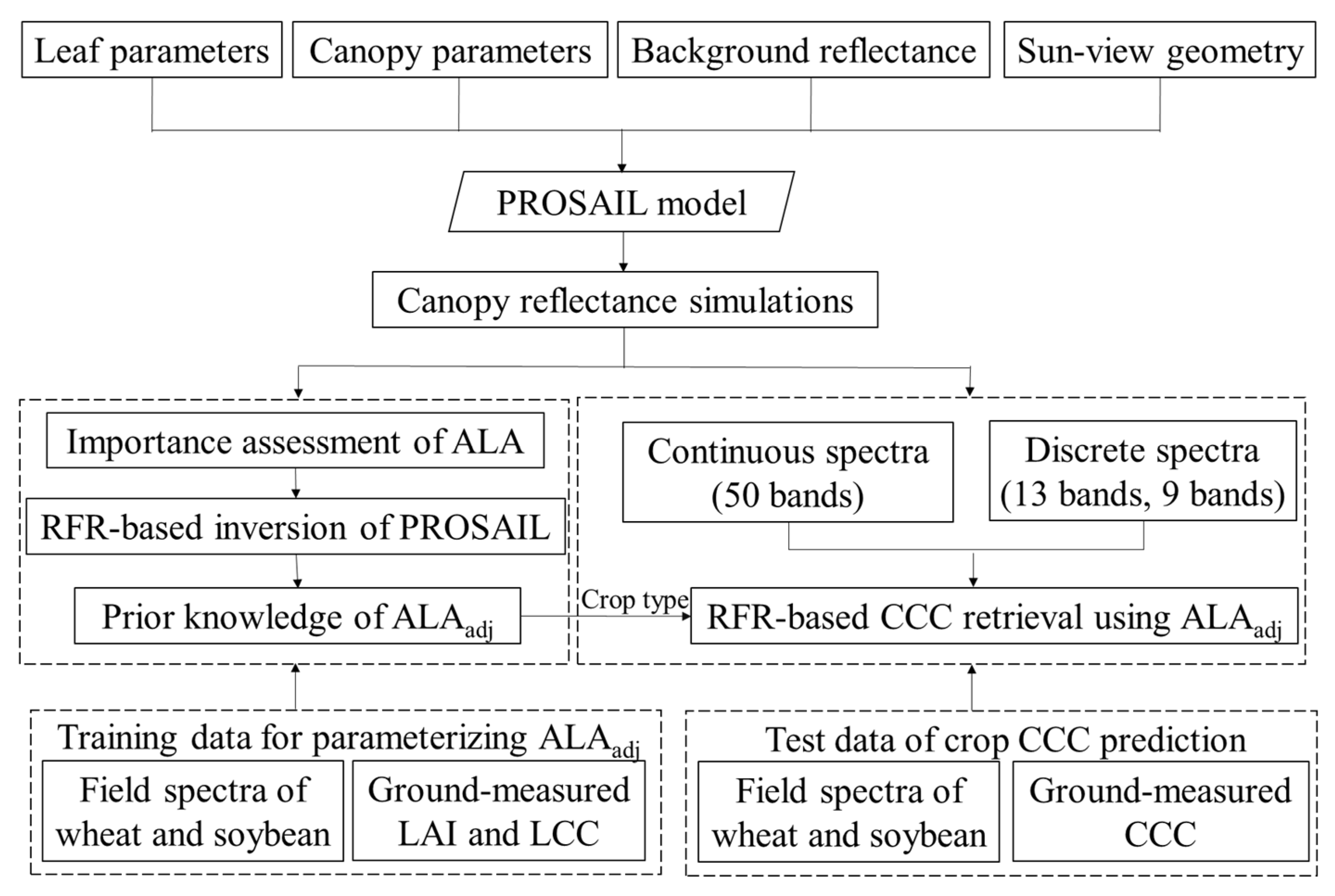
Figure 1. Workflow of crop canopy chlorophyll content (CCC) retrieval and validation methods used in the present study. The prior knowledge of an adjusted average leaf angle (ALAadj) is involved in the PROSAIL-based CCC retrieval model using the random forest regression (RFR) algorithm.
Remotesensing 14 00098 g001
Figure 2. Conceptual effect of ALAadj in (c) on bridging the difference in soil gap fraction cover between (a) a homogeneous canopy case and (b) a heterogeneous canopy case with the same leaf area index (LAI). LAI = LA/A.
Remotesensing 14 00098 g002
Figure 3. Variable importance analysis for canopy reflectance at different wavelengths in the two cases of a homogeneous canopy and vegetation-soil mixed pixels.
Remotesensing 14 00098 g003
Figure 4. Scatter plots of the ground-measured CCC and the CCC predicted by ground-measured canopy spectra, based on the RFR models (ac) without and (d) with prior ALAadj knowledge related to crop types. (a) NonPrior-ALA_45 mode; (b) NonPrior-ALA_62 model; (c) NonPrior-ALA_45_62 model; (d) Prior-ALA_45_62 model.
Remotesensing 14 00098 g004
Figure 5. Scatter plots of the ground-measured and predicted CCC based on the RFR model using continuous and discrete spectra. Above: results of NonPrior-ALA_45_62 model using (a) 50 bands, (b) 13 bands, and (c) nine bands. Below: results of Prior-ALA_45_62 model using (d) 50 bands, (e) 13 bands, and (f) nine bands.
Remotesensing 14 00098 g005
Figure 6. Accuracy of CCC retrieval characterized by LAIs for wheat and soybean using ground-measured continuous spectra (a) without and (b) with considering prior ALAadj knowledge related to crop types. (a) NonPrior-ALA_45_62 model; (b) Prior-ALA_45_62 model.
Remotesensing 14 00098 g006
Figure 7. Applicability of the ALAadj parameterization model for nadir observation to different view zenith angles. The test scenario is a homogeneous canopy simulated by the PROSAIL model, with variations in the view zenith angle and a fixed ALA of 45 degrees. Here, the fixed ALA is equal to the ALAadj truth value.
Remotesensing 14 00098 g007
Table 1. Details of the study sites and statistics of the measured canopy chlorophyll content (CCC, μg cm−2) of wheat and soybean.
SitesLat/Long (°)Crop TypesSampling PeriodsNumberMean CCCStDvCV
BJ-XTS40.18N/116.44EWheat04/02~05/17/2002 and 04/14~05/19/2004 and
04/22~05/13/2019
73147.753.90.365
US-Ne241.17N/−96.47ESoybean06/13~09/17/2002 and 06/29~09/20/200448101.176.50.732
US-Ne341.18N/−96.44ESoybean06/19~09/17/20022571.138.10.727
Lat, latitude; Long, longitude; StDv, standard deviation; CV, coefficient of variation.
Table 2. Configuration of the input parameters for the PROSAIL-D model simulation.
ParametersNameUnitsRange
LeafLCCLeaf chlorophyll contentμg cm−210~80
CmLeaf dry matter contentg cm−20.003~0.006
CbLeaf brown pigment content-0
CwEquivalent water thicknesscm0.02
CarLeaf carotenoid contentμg cm−225% LCC
CantLeaf anthocyanin contentμg cm−22.0
NLeaf structure index-1.0~2.0
CanopyLAILeaf area indexm2 m−20.5~8.0
ALAAverage leaf angledegrees10~80
LIDFbLeaf inclination distribution function parameter b-0
RsoilSoil reflectance-As in Figure S1
hotSHot-spot parameterm m−10.05
θsSolar zenith angledegrees0~60
θvView zenith angledegrees0
φSun sensor azimuth angledegrees0
Table 3. Corresponding band settings of the Envisat MERIS and Sentinel-3 OLCI sensors.
MERIS BandBand CenterBand WidthOLCI BandBand CenterBand Width
B1412.510Oa2412.510
B2442.510Oa3442.510
B349010Oa449010
B451010Oa551010
B556010Oa656010
B662010Oa762010
B766510Oa866510
B8681.257.5Oa10681.257.5
B9708.7510Oa11708.7510
B10753.757.5Oa12753.757.5
B11760.6253.75Oa13761.252.5
B12778.7515Oa16778.7515
B1386520Oa1786520
B1488510Oa1888510
B1590010Oa1990010
The unit of band center and band width is nm.
Table 4. ALAadj (degrees) obtained through PROSAIL parameterization, based on the measured data of wheat and soybean.
Crop TypeUsing SPEC_LAI_LCCUsing SPEC_LAIUsing SPEC_LAI
MeanMeanMeanStDv
Wheat62.05.261.85.262
Soybean45.19.345.79.345
SPEC_LAI, measured data for ALA optimization, including canopy spectra and the measured LAI; SPEC_LAI_LCC, canopy spectra, the measured LAI, and the leaf chlorophyll content (LCC); StDv, standard deviation.
Table 5. Statistical results of the CCC retrieval accuracy for wheat and soybean samples.
MethodWheatSoybeanWheat and Soybean
R2RMSEBiasR2RMSEBiasR2RMSEBias
NonPrior-ALA_450.4856.240.00.8626.9–6.50.6244.116.8
NonPrior-ALA_620.6137.916.60.9248.2–30.40.6543.4–6.9
NonPrior-ALA_45_620.6339.421.60.9140.3–22.70.6739.9–0.5
Prior-ALA_45_620.6137.916.60.8626.9–6.50.7632.95.0
The unit of RMSE and Bias is μg cm−2.
Publisher’s Note: MDPI stays neutral with regard to jurisdictional claims in published maps and institutional affiliations.