Article

Potential of Multiway PLS (N-PLS) Regression Method to Analyse Time-Series of Multispectral Images: A Case Study in Agriculture

1
INRAE, Institut Agro, ITAP, University Montpellier, 34000 Montpellier, France
2
ChemHouse Research Group, 34000 Montpellier, France
3
CNRS, IMS, UMR No. 5218, Groupe Signal et Image, Université de Bordeaux, 33405 Talence, France
4
INRAE, Institut Agro, LISAH, University Montpellier, 34000 Montpellier, France
*
Author to whom correspondence should be addressed.
Remote Sens. 2022, 14(1), 216; https://doi.org/10.3390/rs14010216
Submission received: 2 November 2021 / Revised: 9 December 2021 / Accepted: 28 December 2021 / Published: 4 January 2022

Abstract

:
Recent literature reflects the substantial progress in combining spatial, temporal and spectral capacities for remote sensing applications. As a result, new issues are arising, such as the need for methodologies that can process simultaneously the different dimensions of satellite information. This paper presents PLS regression extended to three-way data in order to integrate multiwavelengths as variables measured at several dates (time-series) and locations with Sentinel-2 at a regional scale. Considering that the multi-collinearity problem is present in remote sensing time-series to estimate one response variable and that the dataset is multidimensional, a multiway partial least squares (N-PLS) regression approach may be relevant to relate image information to ground variables of interest. N-PLS is an extension of the ordinary PLS regression algorithm where the bilinear model of predictors is replaced by a multilinear model. This paper presents a case study within the context of agriculture, conducted on a time-series of Sentinel-2 images covering regional scale scenes of southern France impacted by the heat wave episode that occurred on 28 June 2019. The model has been developed based on available heat wave impact data for 107 vineyard blocks in the Languedoc-Roussillon region and multispectral time-series predictor data for the period May to August 2019. The results validated the effectiveness of the proposed N-PLS method in estimating yield loss from spectral and temporal attributes. The performance of the model was evaluated by the R2 obtained on the prediction set (0.661), and the root mean square of error (RMSE), which was 10.7%. Limitations of the approach when dealing with time-series of large-scale images which represent a source of challenges are discussed; however, the N–PLS regression seems to be a suitable choice for analysing complex multispectral imagery data with different spectral domains and with a clear temporal evolution, such as an extreme weather event.

Graphical Abstract

1. Introduction

Benefiting from the large number of high-quality spectral-temporal images captured from Earth observation satellites, remote-sensing based on multitemporal and multispectral imagery has a great potential to provide timely and comprehensive agricultural and environmental information. With the availability of more and more remote sensing platforms, massive amounts of remotely sensed data are produced [1]; for example, every 5 days, the Sentinel-2 multispectral satellite constellation can provide a global coverage of Earth’s land surface. According to Bovolo et al. [2], new policies for the free distribution of satellites data, the distribution of archive data that makes large-scale retrospective analysis possible, and the increasing number of satellites with higher revisit frequency, are the main reasons for the growing importance of a need for methodological research on multitemporal data analysis.
These large amounts of available remote sensing data have largely been applied to hazard assessment, coastal applications, agricultural applications, natural resource management, etc. [3]. In the field of agriculture, repetitive information on crop status throughout the season at different scales and for different actors, provides the capacity to assist the adaptive evolution of agricultural practices [4]. Chen et al. [5] summarized six main applications of remote sensing in agriculture management and monitoring. For all of these applications, the information of interest consists of traits or features of the agricultural systems, and especially how these vary in space and time. Since plant growth and plant developmental processes are strongly influenced by fluctuations in environmental conditions, and especially ambient temperature [6], capturing the dynamics of crop growth over time, especially at critical growth stages is crucial. Physiological and physical properties of the production system, and consequently the reflectance spectrum, change according to growth conditions, and time of measurement [7]. Consequently, remotely sensed data, obtained by satellites over the time, can provide a set of detailed data on plant growth and development [8].
Regardless of the applications, different approaches to deal with the increasing volumes of data and variables of interest can be found in the remote sensing literature. As Dorigo et al. [9] state in their review, regression methods constitute a widely used tool for explanatory and prediction purposes. When it comes to producing estimates, a popular method to implement this prediction, is the Partial Least Squares method (PLS) [9]. Numerous papers have previously discussed this method from a geometrical, mathematical and statistical point of view [10,11]. PLS methods have been extensively used [12] as they are well-suited to deal with multi-variate data structures with high covariance and redundancy [13], such as are found in remote sensing datasets.
However, challenges remain with respect to addressing these increased data volumes and increased data variability [14]. Exploiting multispectral image time-series is a promising but still relatively underexplored research direction due to the complexity of jointly analysing spatial, spectral and temporal information [15]. The increasing complexity of information leads to a natural generalization of the concept of the ‘data set’ from conventional tables to higher-dimensional arrays [16]. As Bro [17] specified, when including time as an additional dimension, the dataset becomes three-way, which cannot be handled by commonly used conventional prediction models.
Among the alternatives proposed in the literature for modelling multi-way data, deep learning has the potential to outperform traditional classification and regression techniques [18]. However, deep-learning approaches often requires a large dataset to perform the learning and do not provide immediate access to intermediate steps to analyse and understand the agronomic processes that impact production. An interesting alternative to modelling multiway data has been proposed in the chemometrics literature, the multiway partial least squares regression (N-PLS). This is a modelling strategy introduced by Bro [17] and further advanced by Smilde [19]. N-PLS aims at building a model between a high-order array X of independent variables and a response array y [20]. In this paper, PLS regression is extended to multiway data (N-PLS), with the main emphasis on three-way data, by including time as a dimension. It is important to note that N-PLS imposes a trilinear structure on the data [21] and when introducing time into the analysis, this implies that the emphasis is exclusively on the development of a correlational structure over time [22], i.e., time will determine both the variability between individuals and the variability between variables (wavelengths). The N-PLS methodology allows a joint evaluation of time and variables, in order to determine the interaction between them, to know if and how the variables modify their “behaviour” at different occasions. To the authors’ knowledge, such an approach has not been proposed in the analysis of remotely sensed satellite imagery.
Therefore, the objectives of this study are (i) to propose a formalism to apply the N-PLS approach to a time-series of images at the regional scale in order to predict a variable of interest with a small ground truth dataset, (ii) to show the value of the approach for its potential to generate knowledge in an agricultural case study, and (iii) to identify the possible limitations of the approach when dealing with image time-series on large scales with series that may be incomplete for certain areas.
The work is organized as follows: Section 2 introduces the proposed NPL-S method and the development of the model as well as the description of the case study that the methodology is applied to. The results are presented in Section 3, with the discussion in Section 4.

2. Materials and Methods

2.1. Type of Problem the N-Way Partial Least Squares Aims to Address in Remote Sensing

The type of problem that the proposed methodology of this study addresses is the detection of a rapid extreme climate event (frost, hail, heat wave, etc.) that may affect production over a large area (e.g., a regional scale). It is assumed that the extreme climate event has an effect on production by affecting either the pigment content of the leaves, the biomass itself (growth limitation) or the physical architecture of the plants [23]. Therefore, a time-series of multispectral satellite image should provide relevant information to detect the date of occurrence, the severity and also the spatial footprint of the extreme event under study. However, monitoring only a single variable, or only a few variables, is problematic as many variables are correlated and interrelated and have an effect on one another. Consequently, the use of a multidirectional (spectral and temporal) unfolding method (N-PLS) for a given extreme weather event (heat wave) that simultaneously examines all spectral information at different points in time should be well adapted to the challenge of anomaly and event detection in temporal data.
Considering imagery time-series, a fixed classical object/variable scenario, i.e., an agricultural field, can be observed several times under different conditions, yielding a separate data table for each condition [16]. Another option would be to pool all the object/variable conditions together taking into account the time-series of images, which leads to a consideration of a cubic or a three-dimensional data array as shown in Figure 1. Such an array has N images containing the corresponding objects (O) at Tn different dates, with each image being constituted of Mm spectral bands or wavelengths (variables). Given the data dimensionality, multiway arrays have been proven to be a natural and efficient representation of the data, in particular, tensor subspace learning methods have been shown to outperform their corresponding vector subspace methods, especially for small sample size problems [24]. Therefore, the N-PLS algorithm should constitute a relevant approach to retrieve the information contained in the spectral bands of satellite imagery to highlight the target phenomenon taking into account its effect on the temporal evolution of the imagery.

2.2. N-Way Partial Least Squares

In general, the PLS approach is particularly useful when one or a set of dependent variables needs to be predicted by a (very) large set of predictor variables (or time-series) that are strongly cross-correlated [25]. The strength of N-PLS is that it summarizes all latent information from a large 3-way dataset of object variables (X) and relates it to a dependent variable (y) using a relatively low number of parameters, which makes the prediction more robust [26]. This situation leads to an analysis that is able to extract the maximum information possible from samples measured at different times based on cubic structure.
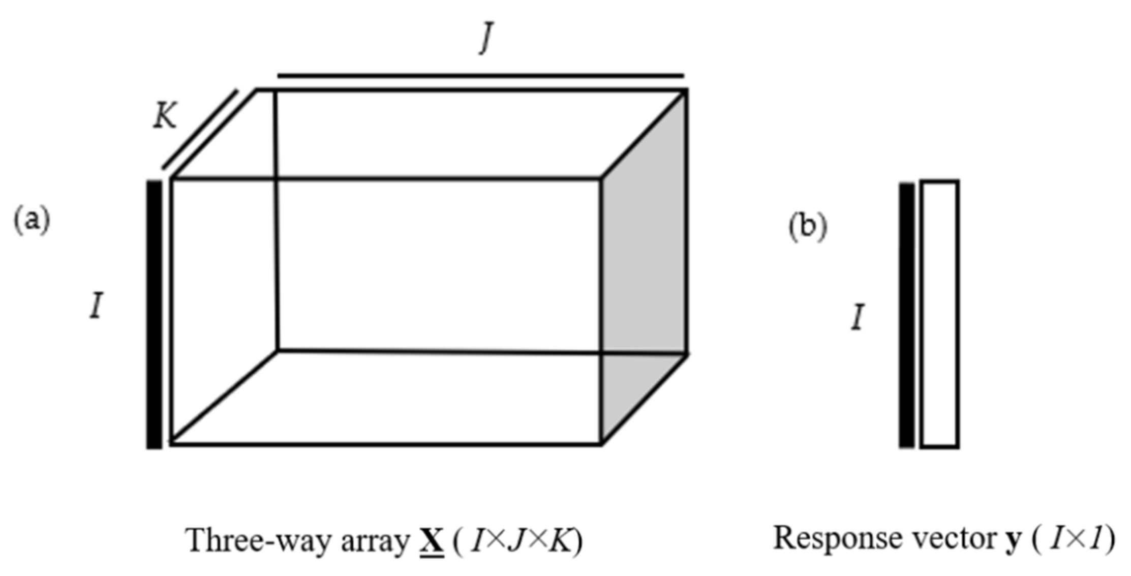
For these remote sensing data, the 3-PLS1 method [17] was considered here to generate a three-way array X = ||Xi,j,k||. The first of the three dimensions of cube X corresponds to the objects (I), the second to time (J) and the third to spectral bands (K). Thus, the data were organized in a three-way array of independent variables X (I × J × K) and a response vector y of size (I × 1) that is defined by the objects dimensions (Figure 2).
The N–PLS regression was used to relate the three-way array X (remote sensing data) to the response vector y (ground truth data). As Abdi [25] specified, PLS regression performs a simultaneous decomposition of X and y by means of a set of latent variables that explain as much as possible of the covariance between X and y. As Bergant et al. [27] detailed, if X (I × JK) is a properly unfolded two-way form of a three-way array X (I × J × K), the 3-PLS1 method can be written in mathematical form (Equation 1), where X and y are cantered along the first dimension, I.
S = XW y = Sb + r .
Estimating the weight array W, allowing for the scores in S to be expressed directly in terms of the X-columns, is the essential part of the method [28]. The regression coefficients b (Equation (1)) can be estimated afterwards by a least square approach [27]. The vector r in Equation (1) presents the part of y not explained by the model. For the estimation of W, the algorithm for three-way X and a single response y proposed by Jong [28] was considered. If the initial values of y a (a is the latent variable counter) are set to the original values y (a = 0 and y 0 = y ), the algorithm can be summarized as follows [27]:
  • Compute the reshaped covariance matrix Ž = y a T  X (1 × JK).
  • Define the first singular weight vectors w a J and w a K from Z : [ w a J , w a K ] = svd( Z ,1). From hence, store them as additional columns in separate weight arrays WJ = [ w 1 J w a J ] and WK [ w 1 K w a K ].
  • Compute the weight array by a Khatri-Rao product [27,29] so that W = WKWJ. The Khatri-Rao product defined as a column- wise Kronecker product of the two matrices [27] was used to overcome constraints related to multiway arrays decomposition.
  • Calculate S = XW.
  • Calculate the regression coefficients regressing y on S as b = (STS)−1 ST y .
  • Calculate the residuals r = y Sb.
  • Increase a to a + 1 and continue from step 1 to the appropriate description of y . The inclusion of an additional latent variable (a + 1) in the model is terminated when the joint analysis of RMSEC (Root Mean Square Error of Calibration) and RMSECV (Root Mean Square Error of Cross-Validation) [30] indicates overfitting due to sampling variability.
This brief description of the method highlights its interest for the case described in this article. It allows to a simultaneously consideration of the temporal (J) and spectral (K) components while keeping the information carried by these two components in the analysis.

2.3. Model Construction

2.3.1. Structuration of Time-Series Data

In order to build a cubic data structure (objects × time × spectral bands), all spectral bands were re-interpolated on a date grid, regularly spaced over the period of interest, i.e., the period that the extreme climatic event may have impacted crops. The objective was to ensure that the cubic X, had the same number of steps (N days of measurements) to prevent temporal data gaps due to clouds and inconsistent numbers of available satellite images. The interpolation at a date t was performed band-by-band, by a convolution of the chronology measured with a Gaussian filter [31] centred on t and with full width at half maximum (P).
Temporally sparse satellite observations, especially for areas that can be affected by cloudy conditions, may not be sufficient for monitoring rapid changes such as some phenological crop stages [32]. Moreover, Hird et al. [33] have demonstrated that there is an impact of varying atmospheric conditions and sun-sensor-surface viewing geometries on satellite-derived time-series. A preliminary sensitivity analysis with a noise reduction approach and given time steps provided information on the sensitivity of the variation of the P and N parameters to interpolation. The parameters P and N involved in the interpolation setting, were optimised by cross validation of 2 blocks repeated 5 times of a N-PLS between cube X and vector y using the calibration dataset (see Section 2.3.2). For this analysis, values of P and N ranged from 10 to 50 and 5 to 30, respectively.

2.3.2. Calibration and Validation of the Model

Calibration and validation subsets were created for model assessment. Considering the size and the potential non-regularity of the distribution of the samples from the dependent variable, a calibration set (3/4) and a validation set (1/4) were defined by the distribution of y, as follows:
  • The vector y was sorted in ascending order.
  • After sorting, every fourth individual was placed in the validation set, the others retained in the calibration set.
The optimal number of latent variables was selected using a cross-validation of 2 blocks repeated 10 times of an N-PLS between the X cube and the y from calibration set. As proposed by Bergant et al. [27], the final calibration fit can be written as in Equation (2).
ŷ = Sb = XWb = XBNPLS + b0.
where ŷ is the vector of estimated responses and b0 the intercept of the linear regression model. The matrix of regression coefficients BNPLS = Wb (Equation (2)) can be used on new data for the estimation of unknown response values. The prediction performance of the empirical model was quantified by the standard coefficient of determination (R2), the bias and the standard error parameters [34,35].

2.4. Case-Study

According to Cogato et al. [23], the increasing frequency of heat wave events represents a severe threat to viticulture because periods of extreme heat may affect grape yields and quality. Thus, the detection of the impact of heat waves on perennial crops from dynamic spectral-temporal features using medium-resolution data, could provide valuable information to identify the possible effects of heat waves on production and the spatial footprint of the phenomena at the regional/national scale. A preliminary study of eight heat waves during the 2016–2017 and 2017–2018 growing seasons, showed that medium-resolution spectral data from Sentinel-2 time-series can provide valuable information on the possible effects of heat waves on grapevines [23]. The N-PLS algorithm should therefore constitute a relevant approach to retrieve the information contained in the spectral bands of the time-series that relates the target phenomenon (heat wave in this case).

2.4.1. Study Area

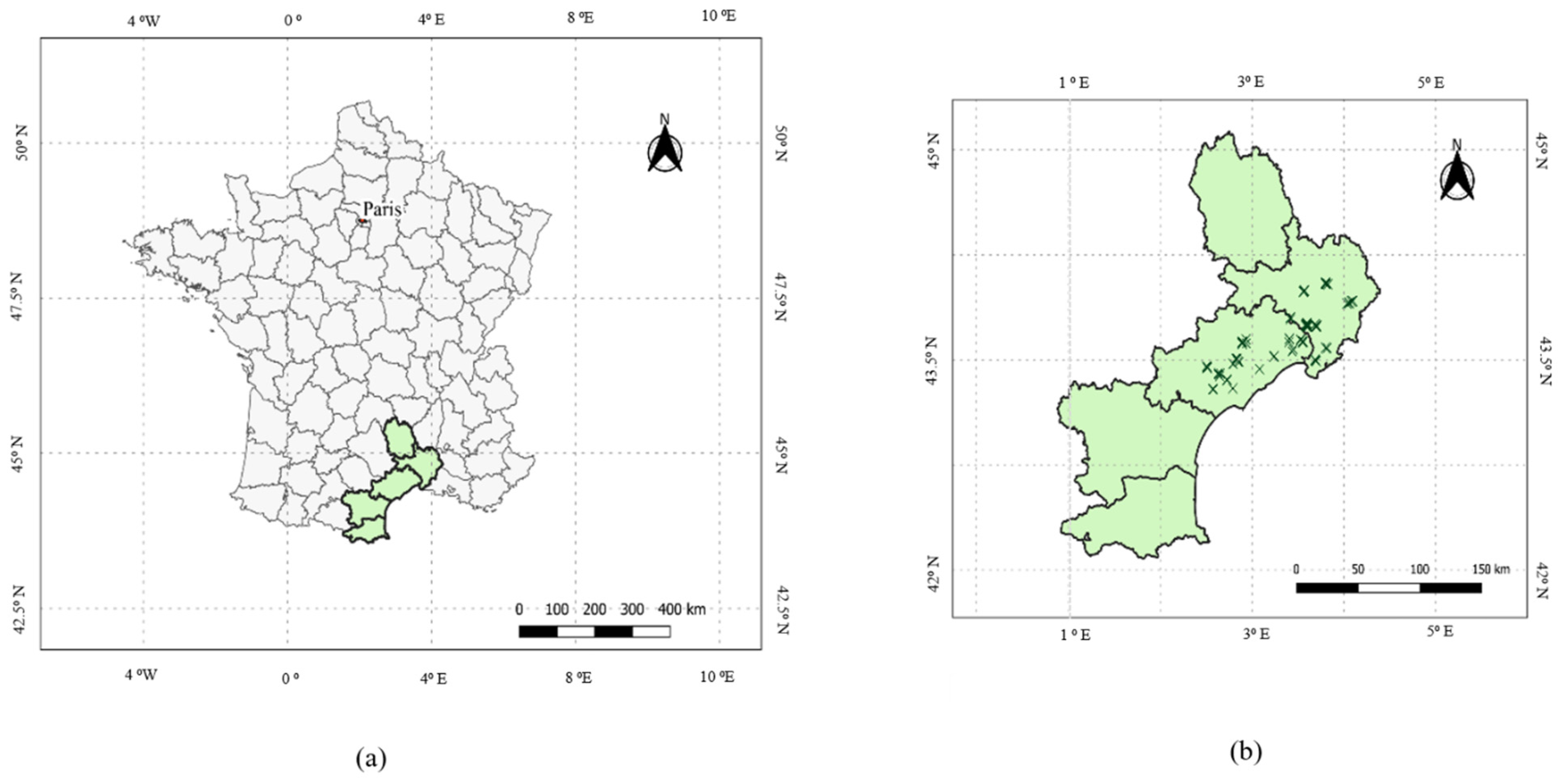
The study area corresponded to a large vine growing region, the Languedoc-Roussillon, located in the south of France (Figure 3). It extends over approximately 27,400 km2, from the Spanish border to the delta of the Rhône.
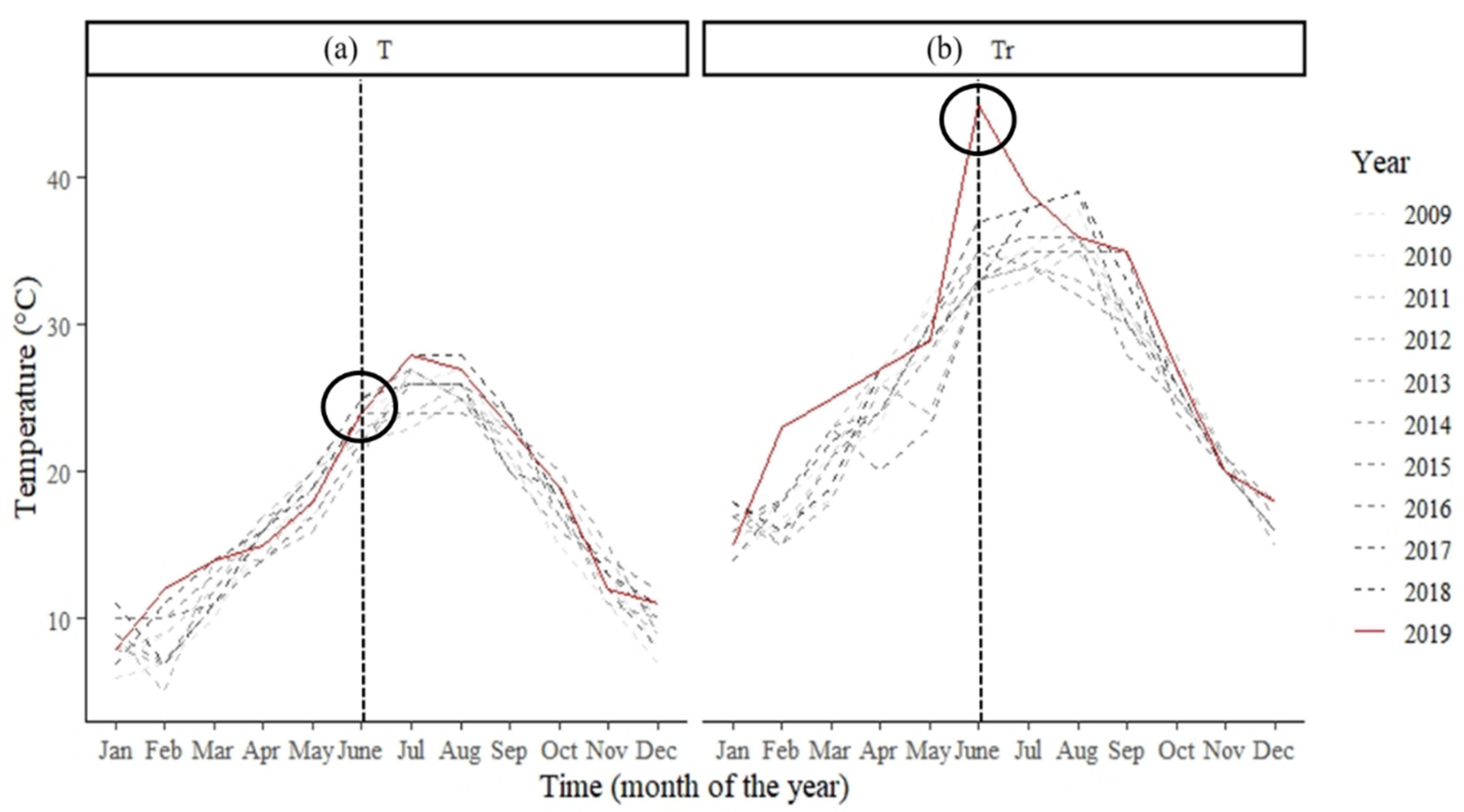
On Friday 28 June 2019, a part of this wine territory experienced an extreme climatic event with a heat wave that reached 45 °C in some places (Figure 4). This heat wave occurred mid-season, that is to say at a critical stage in terms of vine growth.
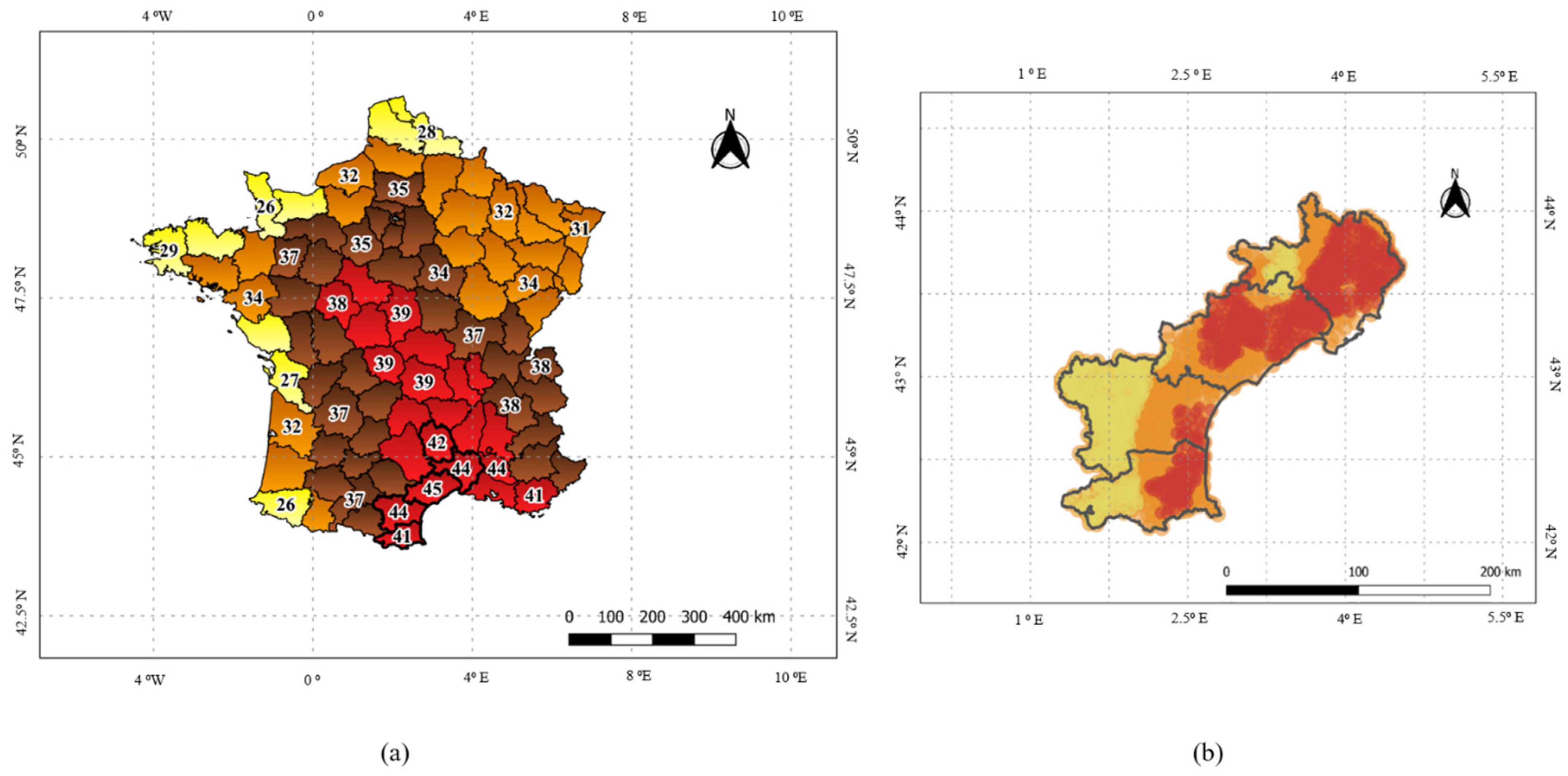
It should also be noted that this extreme heat wave did not affect the entire region but only a part of it, as shown in Figure 5. In addition, the incidence of the heat wave may present a significant spatial variability according to the local elevation, aspect and slope of the individual blocks. The presence of natural features, such as forests or hedges, in the vicinity of the vineyards was also likely to mitigate the effects of the heat wave. This contributed to an observed local variability in the incidence of this climatic event on the vineyard blocks.

2.4.2. Remote Sensing Data

Data Acquisition and Preprocessing

The Sentinel-2 Multispectral Imager is a European Space Agency (ESA) satellite for Earth observation that provides imagery with 13 spectral bands from the near-infrared (NIR) to short-wave infrared (SWIR). The radiometric images are provided with a range of spatial resolutions of 10 m, 20 m and 60 m (Table 1). Each Sentinel-2A or -2B satellite revisits the same area every 10 days (5 days with the twin satellites together).
Images containing the study vineyard blocks (Section 2.4.3) were selected and processed via the Google Earth Engine (GEE) platform that enables large-scale processing of Sentinel-2 L2A (Sentinel-2A and Sentinel-2B) products. The time period considered for the study was from 13th May to 20th August 2019, which is the most relevant period to monitor vine growth vegetation in this region [36]. Following Hollstein et al. [37], decision trees and Bayesian models for cloud detection were applied to the Sentinel-2 images via GEE Javascript API to leave them in ready-to-use formats. Considering the revisit period of the Sentinel-2 (A/B) satellites, 25 images should have been potentially available over each block for the chosen time period. However, after cloud detection, the number of available images for each vineyard was 11 on average, with a range from 7 to 16 images depending on the location of the various vineyards. By using the GEE cloud-based platform to select Sentinel-2 images and pre-process them, the output was a file containing the spectral band values for each date (available images) and for each vineyard block.

Spectral Bands

There were 12 spectral bands (among the 13 available from Sentinel-2 satellites) used in the model (Table 1). Spectral band 10 at 1380 nm was not used as it corresponds to a high atmospheric absorption band dedicated to visible and sub-visible cirrus cloud detection [37]. To avoid mixed pixels, a 10 m inner buffer was imposed at the border of each block to ensure only pure vine pixels were considered. Pure pixels within each block were then averaged for each spectral band at each individual date, i.e., regardless of vineyard block size, each block had one value for each spectral band at a given date.

2.4.3. Ground-Truth Data

The ground-truth data were obtained from 107 vineyard blocks in the Languedoc-Roussillon region (Figure 3). These were all commercial productive blocks with characteristics representative of the Languedoc-Roussillon wine region in terms of plantation density, management practices and diversity of varieties. All blocks were non-irrigated. These blocks were selected because they all showed some effect related to the heat wave, such as stalled development, leaf burn and leaf drop.
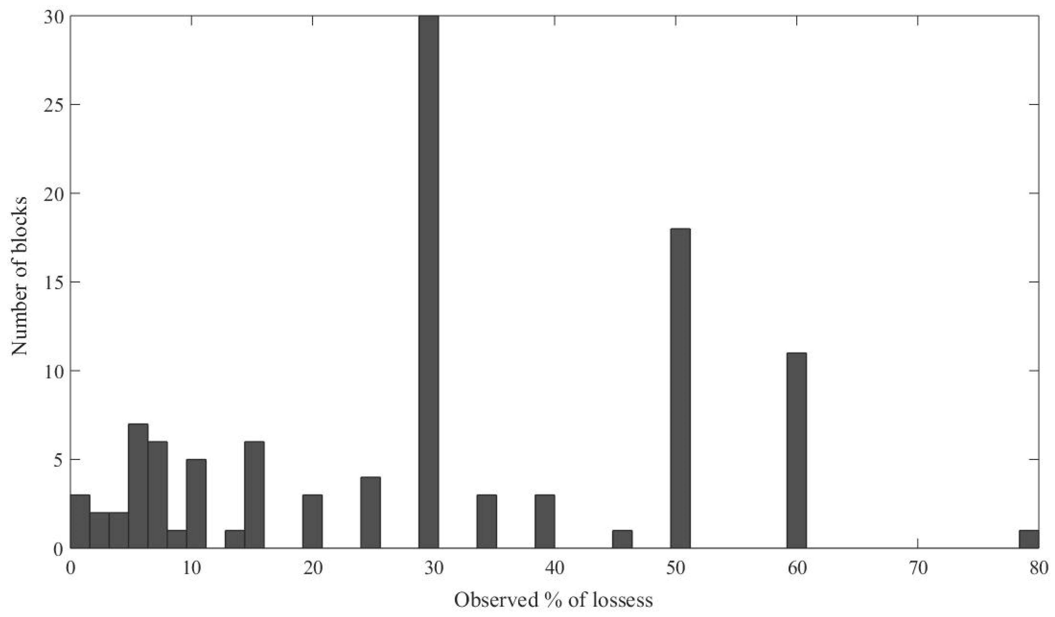
The severity of this effect on each of the 107 vineyard blocks was assessed locally by the winegrowers and advisors. Severity was evaluated several weeks after by an estimation of percentage yield loss. There was an acknowledgement that it was sometimes difficult to attribute the losses to the heat alone. Figure 6 summarizes the distribution of the 107 blocks in relation to estimated yield loss.

2.4.4. Modelling

Model Construction

The final data set was characterized by the repeated observation of 12 spectral bands (variables) averaged for each of the 107 different vine blocks (objects) at 25 potentially available dates over four months (13 May to 20 August), in 2019. This data set was meaningfully arranged in a three-way array X (I × J × K).
As discussed previously, the number of images per block varied according to each block’s geographical location and possible cloud (or other) effects. Thus, X was incomplete and there was a need for interpolation to obtain a continuous data cube. J, defined as the number of dates selected to represent the time-series, can be determined by optimising the parameters N and P. For this model, J was determined by using ranges of N and P described in Section 2.3.1. Once J was determined, interpolation was performed (again following the method in Section 2.3.1) to have a consistent time step.
At the end of the image processing step the data were presented as:
  • a cube X (107, J, 12) where the first dimension corresponds to the vineyard blocks (I), the second dimension corresponds to time (J), which is optimised during modelling, and the third dimension of the three-way array X corresponds to spectral bands (K) averaged for each field,
  • a vector y (107), corresponding to the estimated percentage yield loss by the winegrowers from the 107 blocks.

Model Validation

The calibration and validation subsets were generated using the method outlined in Section 2.3.2. The joint analysis of RMSEC (calibration set) and RMSECV (cross-validation) as proposed by Goodarzi et al. [30] was used to determine the optimal number of latent variables in the regression model.

Model Evaluation

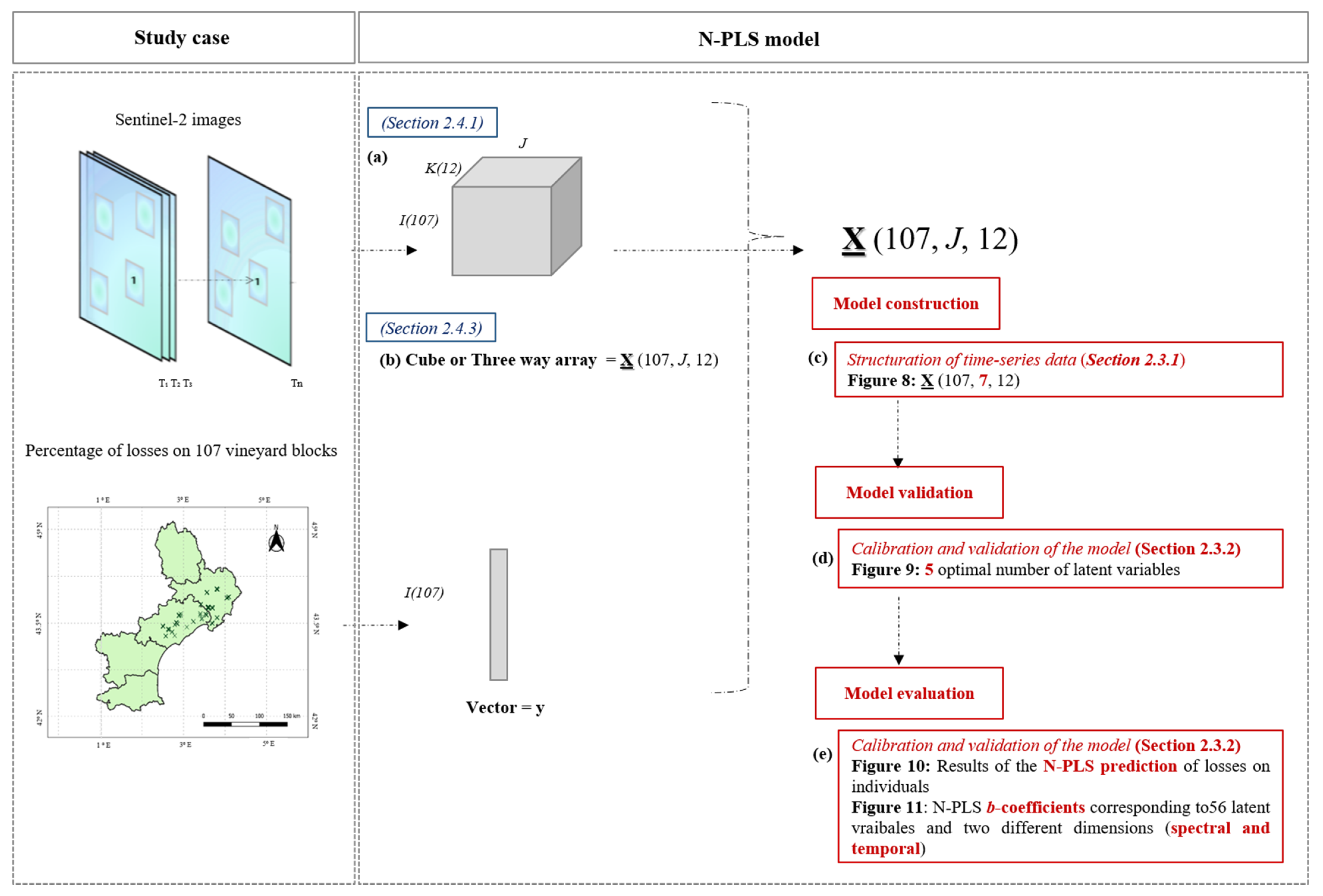
The N-PLS was applied as an approach to detect and characterize the vineyard response (estimated by the percentage of losses) to extreme heat stress by using 12 available reflectance spectral bands from a time-series of Sentinel-2 imagery. As defined in Section 2.3.2, the prediction performance of the N-PLS model was quantified by the standard determination coefficient R2, the bias and the standard error parameters. The regression b-coefficients resulting from the application of the methodology were plotted (i) against time as a function of wavelengths and (ii) against spectral bands as a function of time identify the time and the wavelengths that best highlighted this phenomenon. To further illustrate this, a 3D view of the b-coefficients vs. time vs. spectral bands was also generated. Figure 7 summarizes the implementation and the workflow scheme of the N-PLS adapted to the case study.

3. Results

3.1. Optimisation of Model Parameters over the Study Site

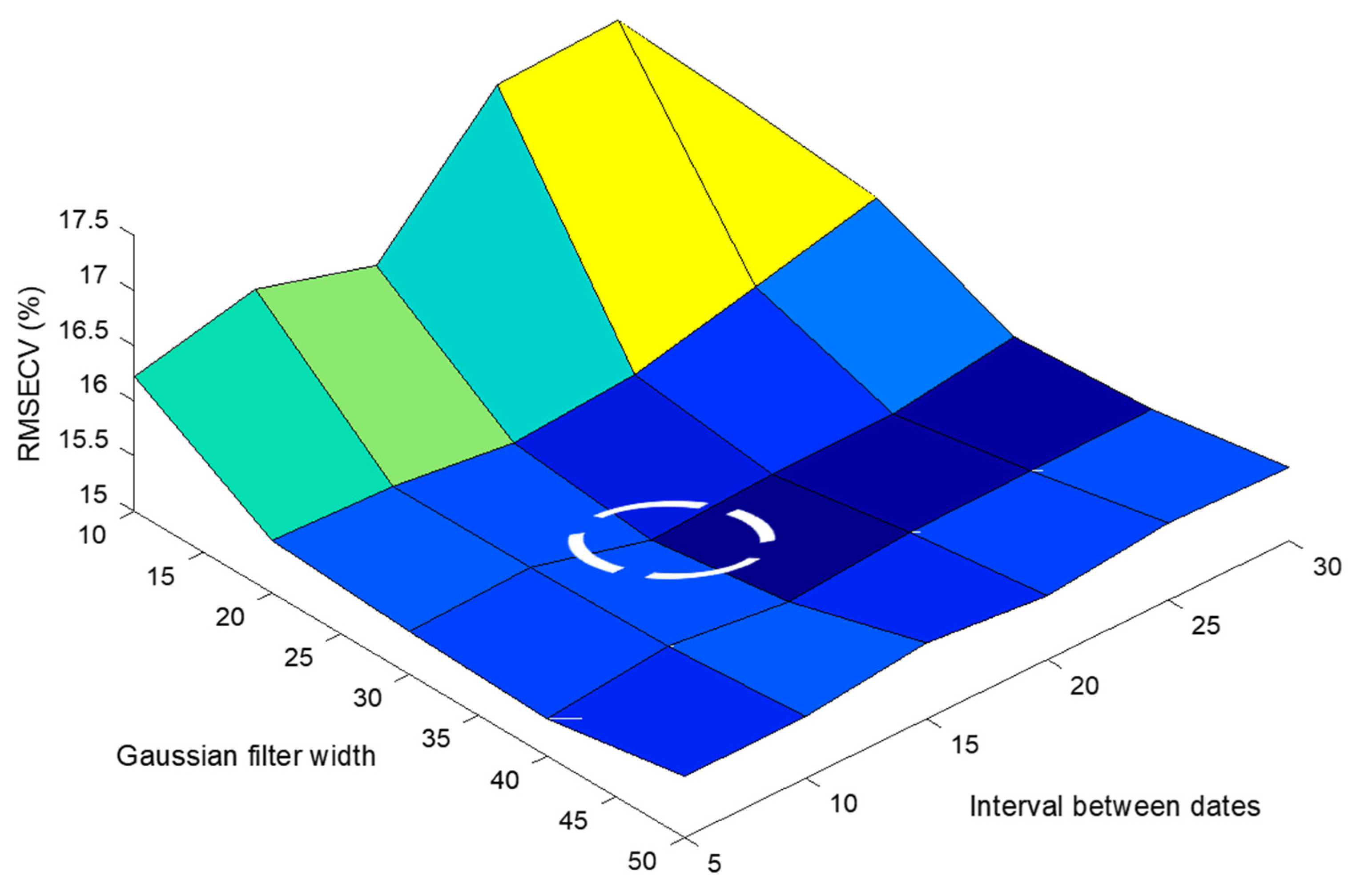
Figure 8 shows the evolution of the RMSECV for a cross-validation of 2 blocks repeated 5 times with a N-PLS performed with the X cube and the y losses from the calibration set when varying the Gaussian filter width (P) and interval between dates (N). This procedure led to an observation of the lowest error of cross-validation (RMSECV) at P = 30 and N = 15. N = 15 equates to J = 7, i.e., 7 dates over the study period, and resulted in a cube X of dimensions (107, 7, 12). Figure 8 highlights three situations in which the cross-validation error (RMSECV) increased when applied to these data, as follows: (i) when the Gaussian filter is too weak (P > 25); (ii) when the time step is short (N < 10 days); (iii) when the time step is long (N > 20 days).
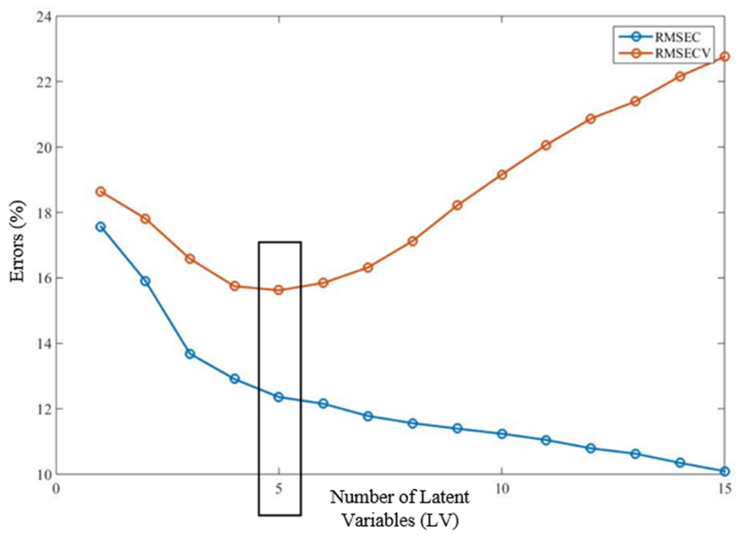
Using the optimised N and P values, Figure 9 presents the evolution of the cross-validation RMSEC and RMSECV against the number of latent variables used in the model. This figure highlighted the following classical phenomenon: a phase of a decrease in the RMSEC, which corresponded to an improvement of the explanatory value of the latent variables, then a phase of increase of the RMSECV (while the RMSEC continued to decrease), which corresponded to the overlearning phase. On the basis of this joint analysis, 5 latent variables were retained for the rest of the study.

3.2. Quality of the N-PLS Model

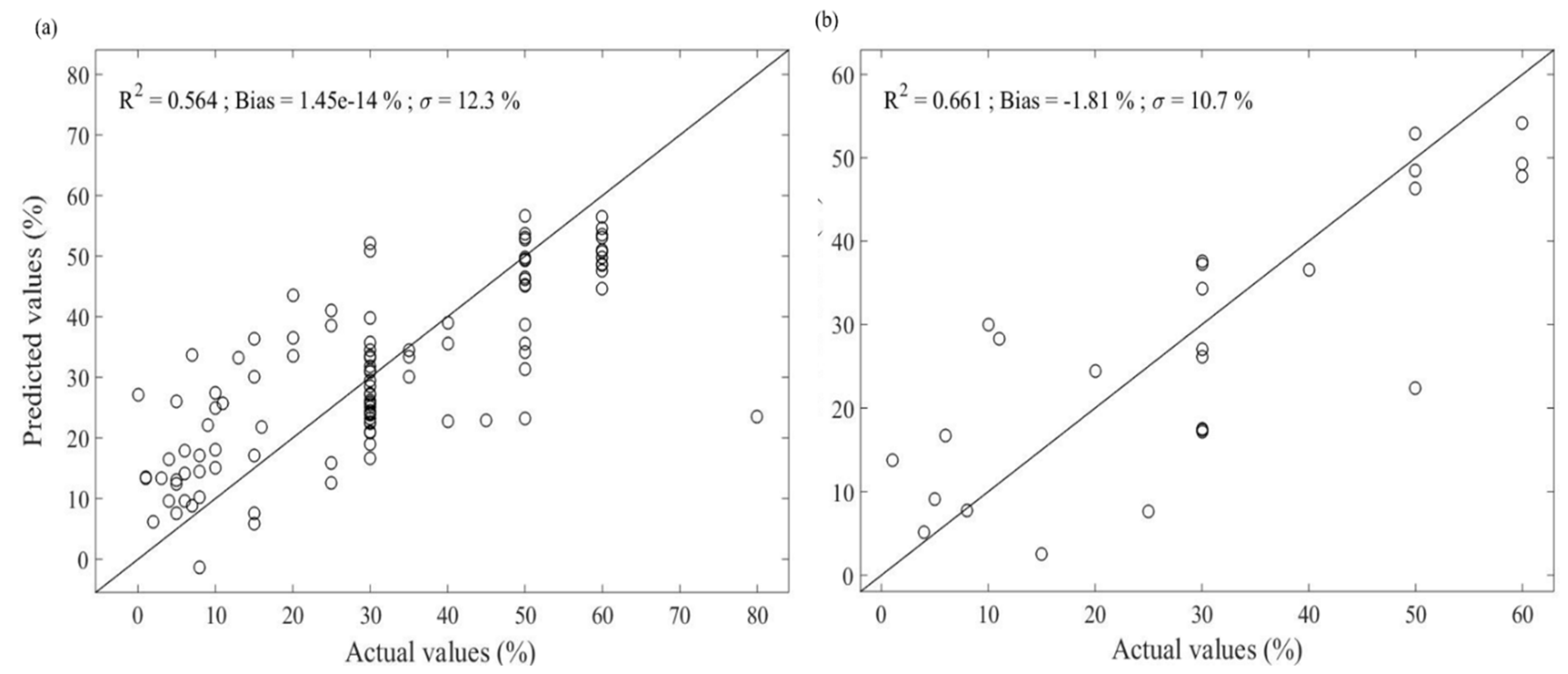
The quality and performance of the N-PLS model with 5 latent variables is presented in terms of R2, the bias and the standard error of prediction of yield losses in the calibration (Figure 10a) and validation (Figure 10b) analyses. The N-PLS model showed a performance accuracy (R2) of 0.56 in the calibration set and 0.66 in the validation set, with a standard error of cross-validation in the calibration set of 12.4% and a standard error of prediction of losses in validation set of 10.7%.
A standard error of prediction over the prediction set of 10.7% (Figure 10b) was consistent with the initial variability of the ground truth data (Section 2.4.3) and also with the information needed by the growers to characterize the level of yield loss in a block that was caused by the heat wave. These results demonstrated the relevance of the approach to detect incidences of heat waves in viticulture and in particular to estimate the yield loss based on spectral and temporal attributes of the images. The results were further validated by the calibration data.
Figure 11 and Figure 12 show plots of the coefficients BNPLS corresponding to the 5 latent variables selected for the model. The N-PLS model estimated yield loss for each block by making the inner product of b-coefficients with a spectral-temporal profile (7 × 12) contained in the cube X (107,7,12). Thus, the b-coefficients had the same dimension as the spectral-temporal profile and could be analysed to identify how specific parts or periods of the spectral-temporal profile were more or less related to yield losses.
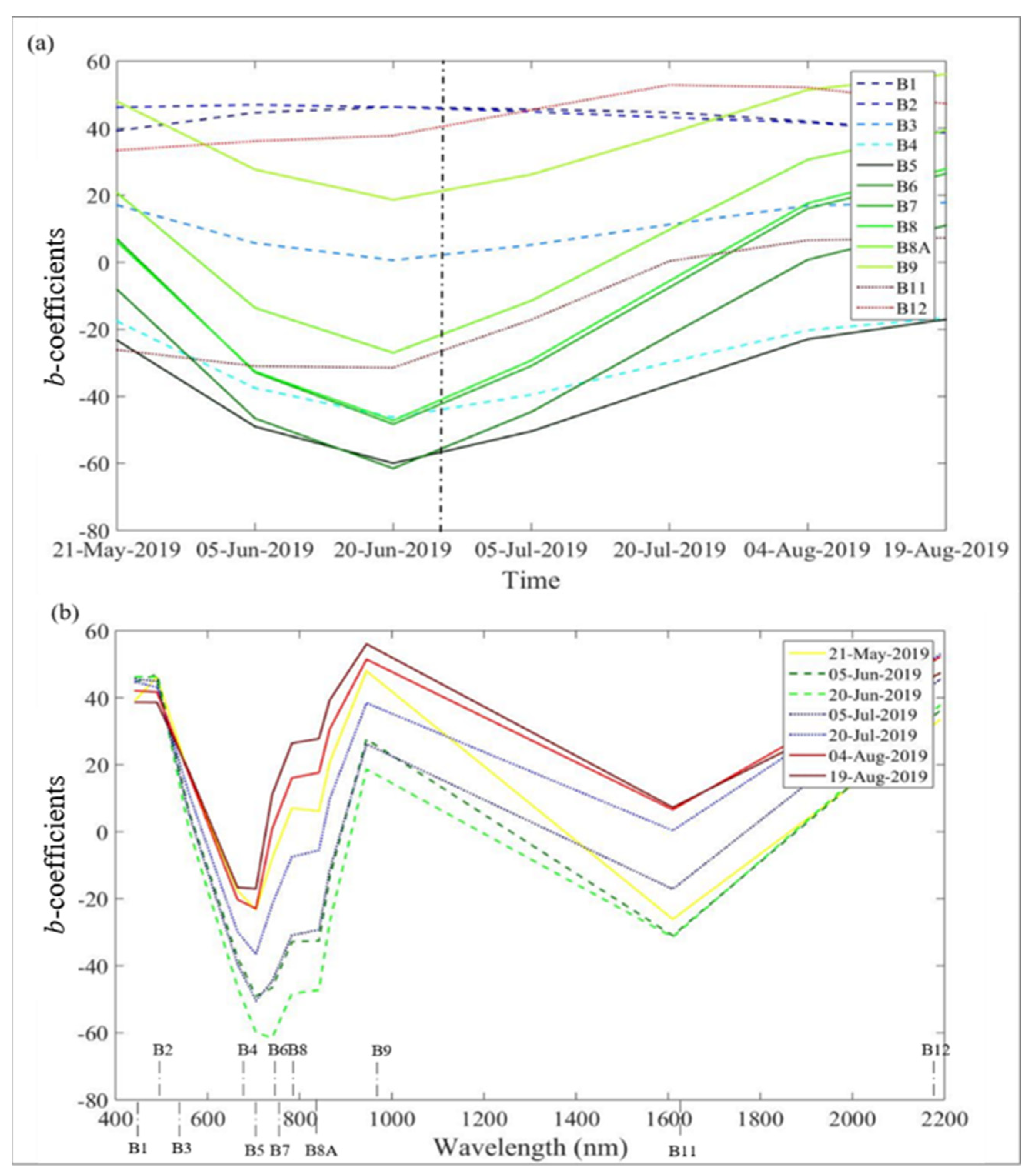
Figure 11 shows the spectral profiles for each spectral band (Figure 11a) and the temporal profiles by date (Figure 11b) of the b-coefficients. Regarding the spectral profile (Figure 11a), the spectral bands were clearly organized into the following three groups: (i) bands B1 and B2 (442.7 and 492.4 nm), which presented no variations throughout the study period, (ii) bands B3, B9 and B12 (559.8, 945.1 and 2202.4 nm), which showed a slight decrease by the end of June and, (iii) the remaining bands B4, B5, B6, B7, B8, B8A and B11 (663.5, 704.1, 740.5, 782.8, 832.8, 864.1 and 1613.1 nm), which presented a very pronounced V-shaped profile with a minimum b-coefficient observed on the 20th of June, identifying these spectral bands as significant in order to identify and characterize the heat stress.
Regarding the temporal profiles (Figure 11b), they were very similar in shape and mainly differed in translation. The higher coefficients were observed for the dates at the beginning and at the end of the study period while the lowest b-coefficients were observed for 20 June, followed by the intermediate dates (5 June and 5 July). The spectral profiles highlighted the end of June as the period that affected on yield loss. Given the interpolation performed, the date of 20 June was the closest to the date of the onset of the heat wave and this date should be considered as the best indicator.
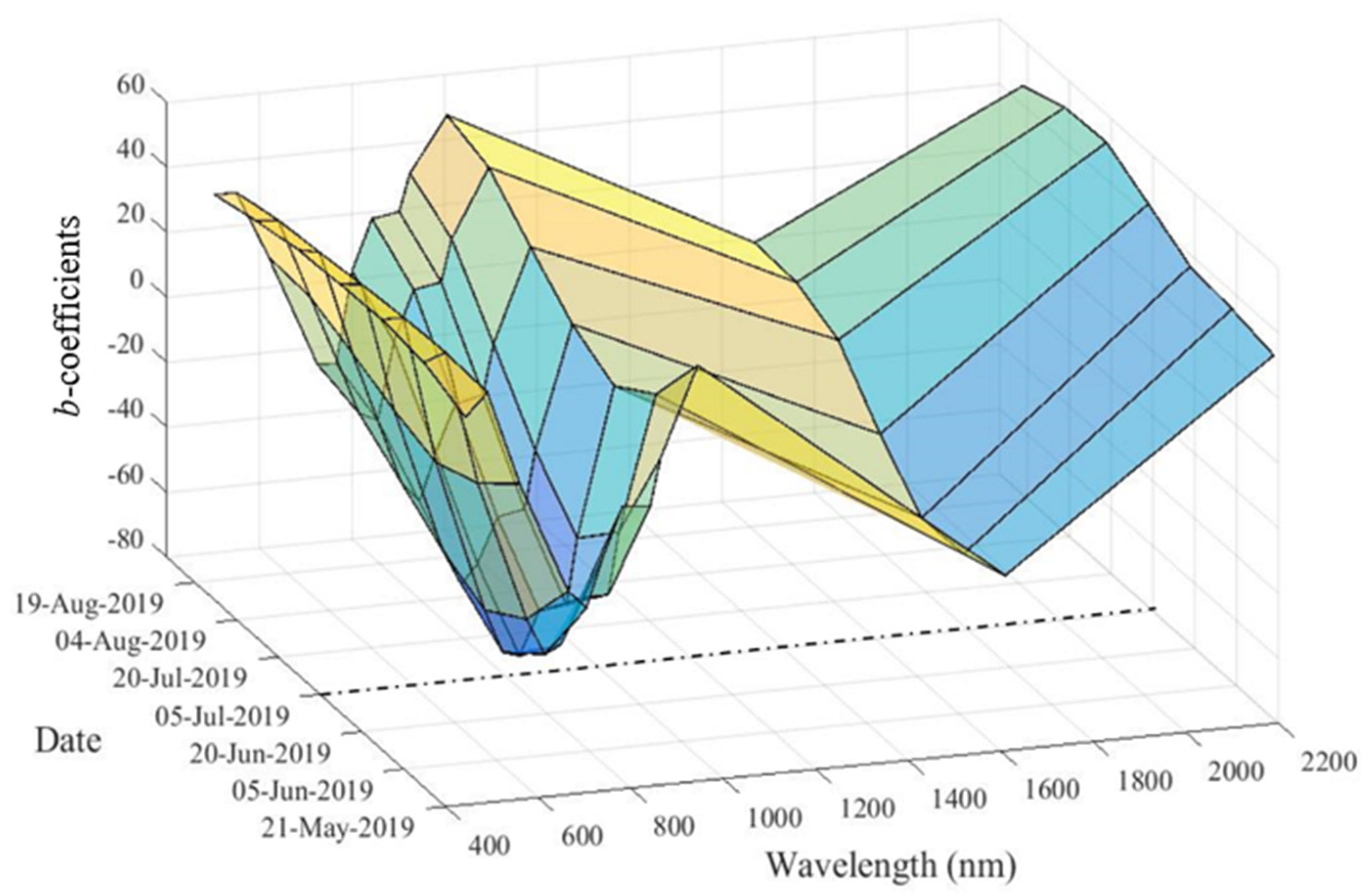
When looking at the b-coefficients, independently from the time dimension, it can be seen that the heat sensitivity was related to a specific spectral shape, with two absorption zones at 700 and 1600 nm (Figure 11b). This spectral shape was close to the typical spectrum of vegetation. It has already been demonstrated that the red edge band has a good potential for estimating plant stress [23]. These results suggested that spectral bands can provide useful information about heat stress in vineyards. By integrating the temporal dimension, it was noticed that the vineyards that suffered most yield loss from the heat wave not only presented a specific spectral shape, but that this spectrum deepened close to the moment of the heat wave (Figure 11a and Figure 12).
Figure 12 combines Figure 11 to shows the 3D shape of the b-coefficients accounting for the spectral and temporal dimension simultaneously.

4. Discussion

A generic example of the application of N-PLS algorithm to time-series of multispectral images was provided in the form of an agricultural study. This paper showed the potential for methods originally developed in the spectrometry/chemometrics domains to be applied to a time-series of Sentinel-2 data. The application showed the value of considering simultaneously the temporal and spectral dimensions with a sensor whose band repartition was partly optimised for vegetation monitoring.
The application of N-PLS to characterize and estimate the impact of an extreme event, such as a heat wave on grapevines, showed that it was possible to predict yield losses with a performance (R2) of 0.66 and a RMSE of approximately 10%. The theory for the use of remote sensing instruments to monitor electromagnetic radiation reflectance changes in crops is well demonstrated in the scientific literature [38]. In situations where crops interact with any given aspect of their environment, such as seasonal climatic variations or meteorological extreme events, the interactions between plants and light reflectance translates into changes in plant signal patterns that can be interpreted using satellite data [39]. Besides the model of yield loss estimation, the N-PLS analysis showed the interest of adopting a systemic analysis which accounts simultaneously for the spectral and temporal characteristics of the considered data. The approach allowed the identification of the spectral bands that responded most strongly to the phenomenon of interest while keeping the information of the period of influence.
Previous studies have reached similar accuracies to assess the effects on heat stress on grapevines [23]. However, notably, the linear nature of the dimensionality reduction in the method presented here allowed for a simple interpretation using the computed b-coefficients, which are directly related to the importance of the explanatory variables, i.e., to the best spectral signature related to the event under study. Since b-coefficients have the same dimension as the spectral-temporal profile, spectral bands around Red Edge (700 nm) and the SWIR region (1600 nm) in late June and early July, were considered relevant to quantify the effect of a heat wave that occurred in late June. It has already been demonstrated that the Red Edge band has a good potential for estimating plant stress, either due to water loss or to leaf pigment modifications [23,40,41]. In particular, this band has been useful for studying how experimental water deficits change the characteristics of plant physiology (e.g., chlorophyll a/b ratio), as plants experiencing a water deficit change their foliar chlorophyll composition, resulting in a shift of red-edge reflectance towards shorter wavelengths [42]. Regarding the shortwave infrared region (SWIR), from approximately 1300 nm to 2500 nm, the absorption of radiation is largely dominated by water [39]. These results generally supported the prediction that wavelengths, where the water absorption coefficient is weak, will penetrate further into canopies and thus will be best for estimations of water content, as is the case in the 1600 nm region [43]. This implied that the SWIR region of the spectrum may potentially be efficient for drought stress detection and resulting changes in canopy tissues [23]. The results of the current analysis confirmed, with a data-driven approach, that a combination of Red Edge and SWIR regions was a valuable indicator in identifying grapevine heat stress on a regional scale.
It is essential to place the results presented in this paper within the reality of multitemporal satellite data. Satellite observations are heavily conditioned by cloud coverage over the acquisition period. Despite this, this method was able to manage a time-series dataset with different sets of missing values by means of an interpolation on a date grid that was regularly spaced and optimised over the period of interest. The N-PLS methodology does not handle a high percentage of missing values within its cubic data structure and, it is expected that this approach would be affected in cases where cloud conditions during the target period significantly limit the number of available images. Another constraint that the model was able to deal with was the low number of ground truth samples (in this case, yield loss observations for grape fields). Note that ground truthing remains cumbersome and difficult to manage for many environmental and agricultural studies. Such limitations can influence the values of model outputs, resulting in a lower reliability of the supervised approach. However, this work showed that N-PLS gave relevant prediction results for a complex phenomenon with a very limited number of data (n = 80) in the calibration data set.
These results indicated that the algorithm may be suited to other similar satellite systems, such as the Landsat products. However, it is important to keep in mind that while the spectral band specifications are similar between the Sentinel and Landsat systems (cross-calibration was actually performed between the two sensors [44]), the Landsat constellation provides imagery with a lower spatial resolution (30 m for most of the spectral bands) which may be a problem for some applications (e.g., intra-field variability in vineyards) but is not crucial for others. The combination of both Landsat and Sentinel-2 products remains a research question [45]. However, such an image combination may be interesting to explore with the N-PLS method in order to foster some limit when working at the regional scale, i.e., missing values due to weather conditions that prevent a full time-series of the objects being studied to be obtained.
While this paper has focused on the monitoring of grapevine heat stress, the identification of the spectral bands that best explain the impact on plant canopy and the development of a local model, which can be applied to predict the spatial extent of the phenomenon, can be transferred to other agricultural applications related to climatic phenomena (e.g., hail or frost). Because of the type of approach, the model should only be valid for the year and the region considered. The resulting model remains specific to the learning base used for the calibration and its generalisation to other vintages and/or other agricultural regions is somewhat limited, especially when dealing with extreme climatic events. However, the results obtained can help facilitate the development of empirical models to be applied to other situations and other vintages.
The type of multi-spectral and multi-temporal method presented in this work is expected to be relevant for any application that relies on different spectral domains with a clear temporal evolution. However, its application to more gradual phenomena, such as progressive changes in plant water status over the summer period, would require further testing, as it may be less relevant because changes in plant characteristics may be less obvious.
In general, the methodology presented here can be effective for any environmental and agricultural application of Sentinel-2 that involves the monitoring of a sharp temporal evolution and where all spectral information may be useful.

5. Conclusions

This study demonstrated how, with a dimensionality reduction algorithm, it is possible to describe the underlying phenomena by highlighting spectral bands and relevant time periods within a time-series of imagery.
This was demonstrated by analysing the footprint of an extreme climatic event and predicting yield losses from a heat wave in 2019 in vineyards in the Languedoc-Roussillon region. In this case, spectral bands around the Red Edge (700 nm) and the SWIR region (1600 nm) were found relevant, as their spectral profile showed a deepening of the time profile during the period of the heat stress, which permitted the band information to be related to reported yield losses.
The proposed method cannot handle temporal data gaps due to clouds and inconsistent availability of satellite images during the acquisition period. Interpolation of the data to achieve a three-way data structure was mandatory for the development of the methodology. By doing this, the method was able to deal with a time-series data set with different sets of missing values and to identify a noise reduction approach with a 15-day time step, which led to a consideration of only seven dates over the study period.
Further investigation is needed to (i) complete the results of this study, expanding the analysis to the spatial distribution of the phenomenon in order to determine its regional dynamics and thus the reasons for its main effects, and to (ii) confirm the applicability of the N-PLS method to different time-evolving phenomena.

Author Contributions

Conceptualization, E.L.-F., G.B. and N.D.; formal analysis, E.L.-F. and J.-M.R.; methodology, E.L.-F., B.G. and M.M.; validation, E.L.-F. and F.R.; writing—original draft preparation, E.L.-F.; writing—review and editing, E.L.-F., B.T. and J.T.; visualization, E.L.-F.; supervision, J.-M.R. All authors have read and agreed to the published version of the manuscript.

Funding

This research received no external funding.

Acknowledgments

The authors would like to thank for the opportunity to have participated in the “Projet Canicule 2019”. This work was supported by the French National Research Agency under the Investments for the Future Program, referred as ANR-16-CONV-0004.

Conflicts of Interest

The authors declare no conflict of interest.

References

  1. Albanwan, H.; Qin, R. A Novel Spectrum Enhancement Technique for Multi-Temporal, Multi-Spectral Data Using Spatial-Temporal Filtering. ISPRS J. Photogramm. Remote Sens. 2018, 142, 51–63. [Google Scholar] [CrossRef]
  2. Bovolo, F.; Bruzzone, L. The Time Variable in Data Fusion: A Change Detection Perspective. IEEE Geosci. Remote Sens. Mag. 2015, 3, 8–26. [Google Scholar] [CrossRef]
  3. Mishra, S.; Shrivastava, P.; Dhurvey, P. Change Detection Techniques in Remote Sensing: A Review. IJWMCIS 2017, 4, 1–8. [Google Scholar] [CrossRef]
  4. Weiss, M.; Jacob, F.; Duveiller, G. Remote Sensing for Agricultural Applications: A Meta-Review. Remote Sens. Environ. 2020, 236, 111402. [Google Scholar] [CrossRef]
  5. Chen, Z.; Li, S.; Ren, J.; Gong, P.; Zhang, M.; Wang, L.; Xiao, S.; Jiang, D. Monitoring and Management of Agriculture with Remote Sensing. In Advances in Land Remote Sensing: System, Modeling, Inversion and Application; Liang, S., Ed.; Springer: Dordrecht, The Netherlands, 2008; pp. 397–421. ISBN 978-1-4020-6450-0. [Google Scholar]
  6. Venios, X.; Korkas, E.; Nisiotou, A.; Banilas, G. Grapevine Responses to Heat Stress and Global Warming. Plants 2020, 9, 1754. [Google Scholar] [CrossRef]
  7. Filella, I.; Serrano, L.; Serra, J.; Peñuelas, J. Evaluating Wheat Nitrogen Status with Canopy Reflectance Indices and Discriminant Analysis. Crop Sci. 1995, 35, 1400–1405. [Google Scholar] [CrossRef]
  8. Plant, R.E.; Munk, D.S.; Roberts, B.R.; Vargas, R.L.; Rains, D.W.; Travis, R.L.; Hutmacher, R.B. Relationships between remotely sensed reflectance data and cotton growth and yield. Trans. ASAE 2000, 43, 535–546. [Google Scholar] [CrossRef]
  9. Dorigo, W.A.; Zurita-Milla, R.; de Wit, A.J.W.; Brazile, J.; Singh, R.; Schaepman, M.E. A Review on Reflective Remote Sensing and Data Assimilation Techniques for Enhanced Agroecosystem Modeling. Int. J. App. Earth Obs. Geoinf. 2007, 9, 165–193. [Google Scholar] [CrossRef]
  10. Dayal, B.S.; MacGregor, J.F. Improved PLS algorithms. J. Chemom. 1997, 11, 73–85. [Google Scholar] [CrossRef]
  11. Phatak, A.; Jong, S.D. The Geometry of Partial Least Squares. J. Chemom. 1997, 11, 311–338. [Google Scholar] [CrossRef]
  12. Arenas-Garcia, J.; Camps-Valls, G. Feature Extraction from Remote Sensing Data Using Kernel Orthonormalized PLS. In Proceedings of the 2007 IEEE International Geoscience and Remote Sensing Symposium, Barcelona, Spain, 23–27 July 2007; pp. 258–261. [Google Scholar]
  13. Abdi, H.; Williams, L. Partial Least Squares Methods: Partial Least Squares Correlation and Partial Least Square Regression. Methods Mol. Biol. 2013, 930, 549–579. [Google Scholar] [CrossRef]
  14. Bishop, M.P. 3.1 Remote Sensing and GIScience in Geomorphology: Introduction and Overview. In Treatise on Geomorphology; Shroder, J.F., Ed.; Academic Press: San Diego, CA, USA, 2013; Volume 3, pp. 1–24. ISBN 978-0-08-088522-3. [Google Scholar]
  15. Mou, L.; Bruzzone, L.; Zhu, X.X. Learning Spectral-Spatial-Temporal Features via a Recurrent Convolutional Neural Network for Change Detection in Multispectral Imagery. IEEE Trans. Geosci. Remote Sens. 2019, 57, 924–935. [Google Scholar] [CrossRef] [Green Version]
  16. Henrion, R. N-Way Principal Component Analysis Theory, Algorithms and Applications. Chemom. Intell. Lab. Syst. 1994, 25, 1–23. [Google Scholar] [CrossRef]
  17. Bro, R. Multiway Calibration. Multilinear PLS. J. Chemom. 1996, 10, 47–61. [Google Scholar] [CrossRef]
  18. Li, S.; Song, W.; Fang, L.; Chen, Y.; Ghamisi, P.; Benediktsson, J.A. Deep Learning for Hyperspectral Image Classification: An Overview. IEEE Trans. Geosci. Remote Sens. 2019, 57, 6690–6709. [Google Scholar] [CrossRef] [Green Version]
  19. Smilde, A.K. Comments on Multilinear PLS. J. Chemom. 1997, 11, 367–377. [Google Scholar] [CrossRef]
  20. Hanafi, M.; Ouertani, S.S.; Boccard, J.; Mazerolles, G.; Rudaz, S. Multi-Way PLS Regression: Monotony Convergence of Tri-Linear PLS2 and Optimality of Parameters. CSDA 2015, 83, 129–139. [Google Scholar] [CrossRef]
  21. Sena, M.M.; Poppi, R.J. N-Way PLS Applied to Simultaneous Spectrophotometric Determination of Acetylsalicylic Acid, Paracetamol and Caffeine. J. Pharm. Biomed. 2004, 34, 27–34. [Google Scholar] [CrossRef]
  22. Coppi, R. An Introduction to Multiway Data and Their Analysis. CSDA 1994, 18, 3–13. [Google Scholar] [CrossRef]
  23. Cogato, A.; Pagay, V.; Marinello, F.; Meggio, F.; Grace, P.; De Antoni Migliorati, M. Assessing the Feasibility of Using Sentinel-2 Imagery to Quantify the Impact of Heatwaves on Irrigated Vineyards. Remote Sens. 2019, 11, 2869. [Google Scholar] [CrossRef] [Green Version]
  24. Zhao, Q.; Caiafa, C.F.; Mandic, D.P.; Zhang, L.; Ball, T.; Schulze-bonhage, A.; Cichocki, A. Multilinear Subspace Regression: An Orthogonal Tensor Decomposition Approach. In Proceedings of the 24th International Conference on Neural Information Processing Systems, Granada, Spain, 12–15 December 2011; Shawe-Taylor, J., Zemel, R.S., Bartlett, P.L., Pereira, F., Weinberger, K.Q., Eds.; Curran Associates, Inc.: New York, NY, USA, 2011. [Google Scholar]
  25. Abdi, H. Partial Least Squares (PLS) Regression. Wiley Interdiscip. Rev. Comput. Stat. 2010, 2, 97–106. [Google Scholar] [CrossRef]
  26. Hansen, P.M.; Jørgensen, J.R.; Thomsen, A. Predicting Grain Yield and Protein Content in Winter Wheat and Spring Barley Using Repeated Canopy Reflectance Measurements and Partial Least Squares Regression. J. Agric. Sci. 2002, 139, 307–318. [Google Scholar] [CrossRef]
  27. Bergant, K.; Kajfež-Bogataj, L. N–PLS Regression as Empirical Downscaling Tool in Climate Change Studies. Theor. Appl. Climatol. 2005, 81, 11–23. [Google Scholar] [CrossRef]
  28. Jong, S. de Regression Coefficients in Multilinear PLS. J. Chemom. 1998, 12, 77–81. [Google Scholar] [CrossRef]
  29. Bro, R.; Smilde, A.; Jong, S.D. On the Difference between Low-Rank and Subspace Approximation: Improved Model for Multi-Linear PLS Regression. Chemom. Intell. Lab. Syst. 2001, 58, 3–13. [Google Scholar] [CrossRef]
  30. Goodarzi, M.; Freitas, M.P. On the Use of PLS and N-PLS in MIA-QSAR: Azole Antifungals. Chemom. Intell. Lab. Syst. 2009, 96, 59–62. [Google Scholar] [CrossRef]
  31. Alam, M.S.; Islam, M.N.; Bal, A.; Karim, M.A. Hyperspectral Target Detection Using Gaussian Filter and Post-Processing. Opt. Lasers Eng. 2008, 46, 817–822. [Google Scholar] [CrossRef]
  32. Wang, Q.; Atkinson, P.M. Spatio-Temporal Fusion for Daily Sentinel-2 Images. Remote Sens. Environ. 2018, 204, 31–42. [Google Scholar] [CrossRef] [Green Version]
  33. Hird, J.N.; McDermid, G.J. Noise Reduction of NDVI Time Series: An Empirical Comparison of Selected Techniques. Remote Sens. Environ. 2009, 113, 248–258. [Google Scholar] [CrossRef]
  34. Fadzlillah, N.A.; Rohman, A.; Ismail, A.; Mustafa, S.; Khatib, A. Application of FTIR-ATR Spectroscopy Coupled with Multivariate Analysis for Rapid Estimation of Butter Adulteration. J. Oleo Sci. 2013, 62, 555–662. [Google Scholar] [CrossRef] [Green Version]
  35. Malegori, C.; Nascimento Marques, E.J.; de Freitas, S.T.; Pimentel, M.F.; Pasquini, C.; Casiraghi, E. Comparing the Analytical Performances of Micro-NIR and FT-NIR Spectrometers in the Evaluation of Acerola Fruit Quality, Using PLS and SVM Regression Algorithms. Talanta 2017, 165, 112–116. [Google Scholar] [CrossRef]
  36. Devaux, N.; Crestey, T.; Leroux, C.; Tisseyre, B. Potential of Sentinel-2 Satellite Images to Monitor Vine Fields Grown at a Territorial Scale. OENO One 2019, 53, 52–59. [Google Scholar] [CrossRef]
  37. Hollstein, A.; Segl, K.; Guanter, L.; Brell, M.; Enesco, M. Ready-to-Use Methods for the Detection of Clouds, Cirrus, Snow, Shadow, Water and Clear Sky Pixels in Sentinel-2 MSI Images. Remote Sens. 2016, 8, 666. [Google Scholar] [CrossRef] [Green Version]
  38. Knipling, E.B. Physical and Physiological Basis for the Reflectance of Visible and Near-Infrared Radiation from Vegetation. Remote Sens. Environ. 1970, 1, 155–159. [Google Scholar] [CrossRef]
  39. Segarra, J.; Buchaillot, M.L.; Araus, J.L.; Kefauver, S.C. Remote Sensing for Precision Agriculture: Sentinel-2 Improved Features and Applications. Agronomy 2020, 10, 641. [Google Scholar] [CrossRef]
  40. Seelig, H.-D.; Hoehn, A.; Stodieck, L.S.; Klaus, D.M.; Adams, W.W.; Emery, W.J. Plant Water Parameters and the Remote Sensing R 1300/R 1450 Leaf Water Index: Controlled Condition Dynamics during the Development of Water Deficit Stress. Irrig. Sci. 2009, 27, 357–365. [Google Scholar] [CrossRef]
  41. Laroche-Pinel, E.; Albughdadi, M.; Duthoit, S.; Chéret, V.; Rousseau, J.; Clenet, H. Understanding Vine Hyperspectral Signature through Different Irrigation Plans: A First Step to Monitor Vineyard Water Status. Remote Sens. 2021, 13, 536. [Google Scholar] [CrossRef]
  42. Easterday, K.; Kislik, C.; Dawson, T.E.; Hogan, S.; Kelly, M. Remotely Sensed Water Limitation in Vegetation: Insights from an Experiment with Unmanned Aerial Vehicles (UAVs). Remote Sens. 2019, 11, 1853. [Google Scholar] [CrossRef] [Green Version]
  43. Sims, D.A.; Gamon, J.A. Estimation of Vegetation Water Content and Photosynthetic Tissue Area from Spectral Reflectance: A Comparison of Indices Based on Liquid Water and Chlorophyll Absorption Features. Remote Sens. Environ. 2003, 84, 526–537. [Google Scholar] [CrossRef]
  44. Claverie, M.; Ju, J.; Masek, J.G.; Dungan, J.L.; Vermote, E.F.; Roger, J.-C.; Skakun, S.V.; Justice, C. The Harmonized Landsat and Sentinel-2 Surface Reflectance Data Set. Remote Sens. Environ. 2018, 219, 145–161. [Google Scholar] [CrossRef]
  45. Quintano, C.; Fernandez-manso, A.; Fernández-Manso, O. Combination of Landsat and Sentinel-2 MSI Data for Initial Assessing of Burn Severity. Int. J. App. Earth Obs. Geoinf. 2018, 64, 221–225. [Google Scholar] [CrossRef]
Figure 1. Production of three-dimensional array from satellite imagery time-series data.
Remotesensing 14 00216 g001
Figure 2. (a) Representation of three-way array (X) and (b) response vector y to compute a tri-linear PLS1 procedure.
Remotesensing 14 00216 g002
Figure 3. Location of the study area in Southern France (a) and the location of the vineyards that contained the 107 blocks of interest for the study (b).
Remotesensing 14 00216 g003
Figure 4. Mean monthly temperature (a) and maximum monthly temperatures records (b) from 2009 to 2019 across the Languedoc-Roussillon region, France, highlighting a peak in the maximum monthly temperature corresponding to the extreme weather event that occurred in June 2019, while the mean monthly temperature for this month was not extreme. The vertical black dashed line highlights the month of the heat wave. Source: Historique Météo-France.
Remotesensing 14 00216 g004
Figure 5. (a) Maximum temperature record map 28 June 2019 France. (b) Maximum temperature record map 28 June 2019 Languedoc-Roussillon. Temperatures ≥ 40 °C are shown in red, temperatures < 40 °C and ≥30 °C are shown in orange and temperatures < 30 °C are shown in yellow. Source: Météo-France.
Remotesensing 14 00216 g005
Figure 6. Percentage of yield losses observed by winegrowers on 107 blocks in southern France.
Remotesensing 14 00216 g006
Figure 7. Workflow scheme of N-PLS application to the case study.
Remotesensing 14 00216 g007
Figure 8. Evolution of RMSECV as a function of varying intervals between dates (N) and Gaussian filter width (P) obtained for 2 blocks repeated 5 times with a N-PLS performed with a X cube and the y yield losses. Parameter optimisation was achieved at, P = 30 and N = 15 as indicated by the white dash circle.
Remotesensing 14 00216 g008
Figure 9. Evolution of the RMSEC and the RMSECV for a cross-validation of 2 blocks repeated 10 times of a N-PLS between the X cube and the y losses. The black frame indicates the optimal number of latent variables (5 LV).
Remotesensing 14 00216 g009
Figure 10. Results of the N-PLS prediction of losses on individuals in the calibration set (a), with 80 vineyard blocks and in the validation test (b), with 27 vineyard blocks. The standard error of cross-validation in the calibration set was 12.4 and the standard error of prediction of yield losses in validation set was 10.7.
Remotesensing 14 00216 g010
Figure 11. N-PLS b-coefficients corresponding to 5 latent variables and the following two different dimensions: (a) plotted according to the spectral dimension and (b) plotted according to the temporal dimension. Black dot-dash line highlights the most relevant date of the heat wave.
Remotesensing 14 00216 g011
Figure 12. Combined representation of the temporal and spectral profiles as a 3D view of N-PLS b-coefficients corresponding to 5 latent variables. Black dot-dash line to highlight the most relevant date of the heat wave.
Remotesensing 14 00216 g012
Table 1. Spectral bands for the Sentinel-2 satellite considered by the analysis.
Sentinel-2 BandCentral Wavelength (nm)Bandwidth (nm)Spatial Resolution (m)
Band 1–Aerosol442.72160
Band 2–Blue492.46610
Band 3–Green559.83610
Band 4–Red664.63110
Band 5–Vegetation Red Edge704.11520
Band 6–Vegetation Red Edge740.51520
Band 7–Vegetation Red Edge782.82020
Band 8–NIR832.810610
Band 8A–Vegetation Red Edge864.12120
Band 9–VNIR945.12060
Band 11–SWIR1613.19120
Band 12–SWIR2202.417520
Publisher’s Note: MDPI stays neutral with regard to jurisdictional claims in published maps and institutional affiliations.