Abstract
Many studies have reported that there is a coupling mechanism between ionosphere and earthquake (EQ). Ionospheric anomalies in the form of abnormal increases and decreases of ionospheric Total Electron Content (TEC) are even regarded as precursors to EQs. In this paper, TEC anomalies associated with three major EQs were investigated by Global Ionospheric Maps (GIMs) and GPS-TEC, including Kumamoto-shi, Japan—EQ occurred on 15 April 2016 with Mw = 7.0; Jinghe, China—EQ occurred on 8 August 2017 with Mw = 6.3; and Lagunas, Peru—EQ occurred on 26 May 2019 with Mw = 8.0. It was found that the negative ionospheric anomalies linger above or near the epicenter for 4–10 h on the day of the EQ. For each EQ, the 10-min sampling interval of TEC was extracted from three permanent GPS stations around the epicenter within 10 days before and after the EQ. Variations of TEC manifest that the negative ionospheric anomalies first appear 10 days before the EQ. From 5 days before to 2 days after the main shock, the negative ionospheric anomalies were more prominent than the other days, with the amplitude of negative ionospheric anomaly reaching −3 TECu and the relative ionospheric anomaly exceeding 20%. In case of Kumamoto-shi EQ, the solar-geomagnetic conditions were not quiet (Dst < −30 nT, Kp > 4, and F10.7 > 100 SFU) on the suspected EQ days. We discussed the differences between ionospheric anomalies caused by active solar-geomagnetic conditions and EQ. Combining the analysis results of Jinghe EQ and Lagunas EQ, under quiet solar-geomagnetic conditions (Dst > −30 nT, Kp < 4, and F10.7 < 100 SFU), it can be found that TEC responds to various solar-geomagnetic conditions and EQ differently. The negative ionospheric anomalies could be considered as significant signals of upcoming EQs. These anomalies under different solar-geomagnetic conditions may be effective to link the lithosphere and ionosphere in severe seismic zones to detect EQ precursors before future EQs.
1. Introduction
Since the study of Leonard and Barnes [1] discovered that there is a potential coupling mechanism between earthquake (EQ) and abnormal ionospheric disturbance from the Alaska EQ in 1964, several researches have been devoted to detect short- and long-term seismo-ionospheric anomalies from ionospheric remote sensing measures. Variations in electrical resistivity; the greatest plasma frequency in the ionosphere, foF2; electromagnetism (EM); and ionospheric Total Electron Content (TEC) were correlated with large amounts of energy released during the EQ incubation period, which are probably signs of a impending main shock [2,3,4,5]. TEC can be obtained by dual-frequency, satellite-based measurements from Global Positioning System (GPS) [6]. A large number of published studies have reported that anomalous TEC variations appear either as precursory effects from a few days to a few weeks before an EQ or as late effect around the main shock [7,8]. For example, during the 27-day period before the EQ, negative and positive anomalies appeared in the ionosphere, which were not related to active solar-geomagnetic conditions [9]. Statistical analysis of 10 days of TEC data before global Mw ≥ 6.0 EQs during 1998–2014 showed that within 5 days before the EQs, the positive and negative ionospheric anomalies were the most prominent [10]. Similarly, significant ionospheric TEC depletions were observed 3–4 days before the Chi-Chi EQ—Mw = 7.6—occurred in Taiwan and were different from the equatorial positive anomalies, which were placed on each side of the equator [11]. However, local conditions of the ionosphere are subject to numerous influences such as solar radiation, geomagnetic activity, meteorological events, anthropogenic effects, atmospheric gravity waves (AGW), and traveling ionospheric disturbances (TID) [12,13,14]. When the surroundings of EQ suffer from abnormal space weather effects, with GPS it is difficult to accurately detect the ionospheric TEC anomaly information [12,15]. Thomas et al. [16] even strongly stated that it is impossible to take pre-earthquake ionospheric anomalies as EQ precursor information according to long-term statistical analysis.
Nevertheless, several published researches have reported that solar-geomagnetic activity and other inducements of ionospheric anomalies lead to variability in the ionosphere. There are temporal and spatial characteristics of ionospheric anomalies induced by EQ, which provides an opportunity for us to study ionospheric precursors [15,17,18]. To explain the characteristics, the process of EQ-affected ionosphere has been widely reported. Tectonic forces inside the Earth are the main cause of EQ. The highly active free-electron carrier is activated in the squeezed rocks within seismogenic zones, and they propagate upwards. The rise of conductivity in the air induced by the active free electron, eventually causing ionospheric perturbations [19]. Similarly, Kuo et al. [20] proposed that the deformation of the earth’s surface will cause a change in the magnetic field, and the resulting electric field will have a significant impact on the ionosphere. In other studies, Pulinets et al. [12] proposed a Lithosphere–Atmosphere–Ionosphere Coupling (LAIC) model to explain variations in the atmosphere and ionosphere parameters during the seismic incubation period, showing that the decrease or increase in the thermal conductivity of atmosphere is caused by continuous Radon gas emission from the EQ breed zone.
In this paper, the research of seismo-ionospheric anomalies before three earthquake cases in different regions, with different focal depths and under different solar-geomagnetic conditions was implemented. We analyzed the temporal and spatial distribution of ionospheric anomalies associated with three Mw > 6.0 EQs on the day of each EQ. The temporal series of Vertical Total Electron Content (VTEC) was retrieved from permanent GPS stations within the EQ breed zone from 10 days before to 10 days after the EQ. Sliding interquartile range method was used to distinguish seismo-ionospheric anomalies specifically triggered by the impending main shock. The ionospheric TEC variation related to solar-geomagnetic conditions were discussed in detail with enough evidences. Section 2 introduces the materials and methods; then, Section 3 shows our results and description. In Section 4, we summarize the characteristics of seismo-ionospheric anomalies. The process of EQ-induced ionospheric anomalies is also discussed in detail with previous studies. Finally, in Section 5, our conclusions are provided.
2. Materials and Methods
2.1. Earthquake Data
In this paper, we studied the temporal and spatial TEC anomalies related to three Mw > 6.0 EQs, including the Kumamoto-shi, Japan EQ that occurred on 15 April 2016 with Mw = 7.0; the Jinghe, China EQ that occurred on 8 August 2017 with Mw = 6.3; and the Lagunas, Peru EQ that occurred on 26 May 2019 with Mw = 8.0. They occurred in different locations around the world and under various geomagnetic conditions. EQ occurrence time is converted to Coordinated Universal Time (UTC). The detailed information of these three EQs retrieved from the U.S. Geological Survey (USGS) via http://www.earthquake.usgs.gov/earthquakes/search (accessed on 5 November 2021) is shown in Table 1.

Table 1.
Detailed earthquake information.
2.2. Solar-Geomagnetic Data
In order to distinguish whether ionospheric anomalies are induced by geomagnetic activities, enhanced solar radiation, or seismic processes, we performed statistical analysis on three parameters—Dst, Kp, and F10.7. Dst and Kp indices were obtained from the International Service of Geomagnetic Indices (ISGI) via http://isgi.unistra.fr (accessed on 5 November 2021). The Dst index denotes the global magnetic activity by measuring the intensity of the Earth’s equatorial electrojet. The ranges of −50 nT < Dst ≤ −30 nT, −100 nT < Dst ≤ −50 nT, −200 nT < Dst ≤ −100 nT, and Dst ≤ −200 nT signify small, moderate, large, and strong geomagnetic storms, respectively [21]. The geomagnetic, three-hourly Kp index was derived from the 13 magnetic observatories distributed globally; in the range of 0–9, where 0–2, 3–4, 5, 6, and 7–9, it denotes quiet, unstable, small, large, and severe geomagnetic activities, respectively [22]. The solar radiation index F10.7 obtained from the Space Physics Data Facility (SPDF) via https://omniweb.gsfc.nasa.gov/form/dx1.html (accessed on 5 November 2021), is an indicator of solar activity with 1 h temporal resolution. In the ranges of 70–100 SFU, 100–150 SFU, and 150–250 SFU, it represents low, moderate, and high levels of solar activity, respectively [21].
2.3. GIMs and GPS-TEC Data
Many scientists have utilized GIM containing grid data of the Vertical Total Electron Content (VTEC) to investigate ionospheric phenomena. The GIM is generated by data collected from almost 400 stations distributed around the world, with a temporal resolution of 1 h and spatial resolution of 2.5° × 5° (lat. × lon.) [23]. Preseismic ionospheric anomalies were investigated by GIMs acquired from the Center for Orbit Determination in Europe (CODE) via http://ftp.aiub.unibe.ch/CODE/ (accessed on 5 November 2021), which is one of the most reliable Data Products when monitoring ionosphere [24]. The VTEC retrieved from permanent GPS ground-stations has higher accuracy and temporal resolution. For each EQ, three available GPS stations were selected by the method proposed by Dobrovolsky et al. [25]. The EQ breed zones were estimated by the following equation:
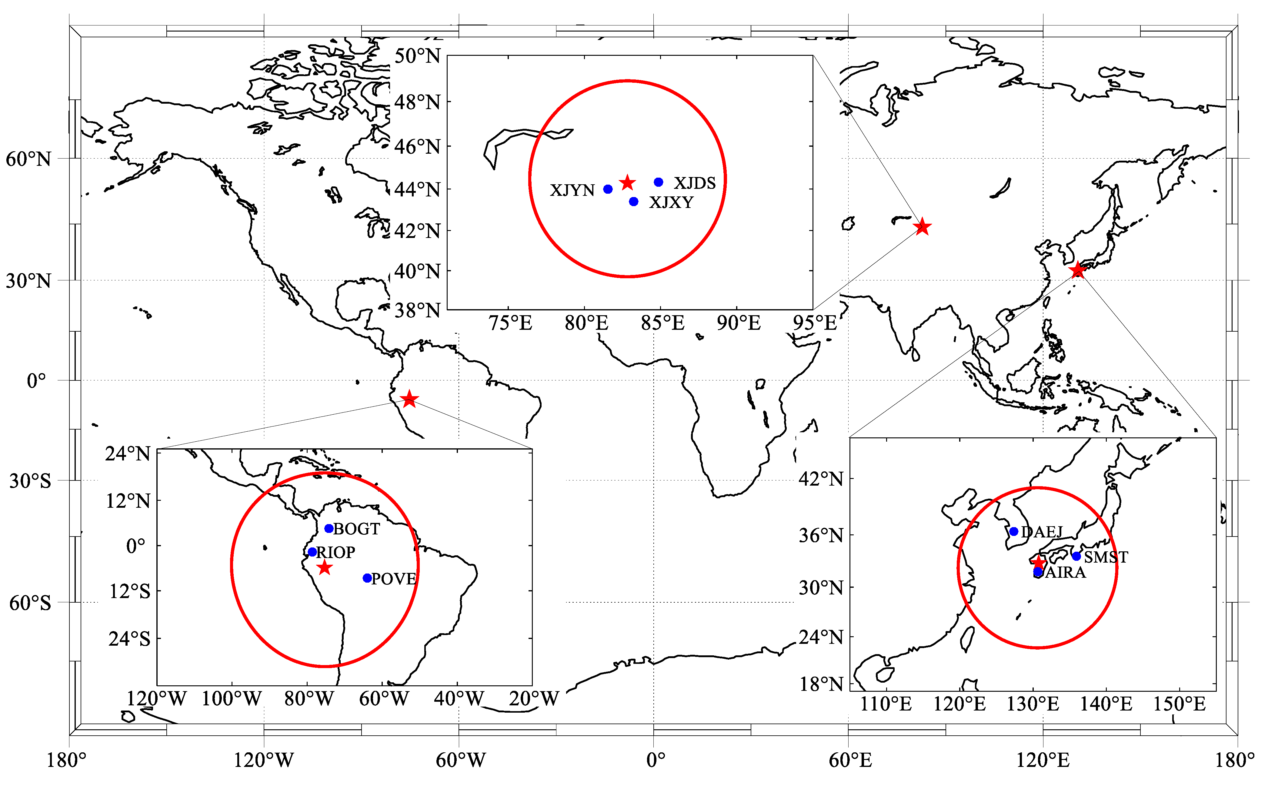
where is EQ magnitude and R is the EQ breed zone’s radius. In this study, all the stations operated within the EQ breed zone are shown in Figure 1.
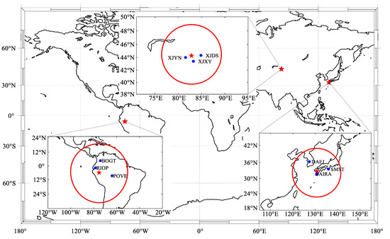
Figure 1.
Geographical location of the three EQs. The epicenters are presented by red stars. The GPS ground-stations are presented by blue dots.
RINEX data of permanent GPS observatories in China (XJDS, XJXY, XJYN) were obtained from the Crustal Movement Observation Network of China (CMONOC), which includes GNSS stations across mainland China and enables the continuous monitoring of the ionosphere over China as accurately as possible [26]. The rest (AIRA, DAEJ, SMST, BOGT, POVE, RIOP) were obtained from International GNSS services (IGS) observatories via http://www.igs.gnsswhu.cn/index.php/Home/DataProduct/igs.html (accessed on 5 November 2021). We extracted the ionospheric VTEC of each site with 10 min sampling intervals. According to the research of Liu et al. [11] and Shah and Jin [10], the 10 days before and after the EQ were selected as EQ-related days.
The main part of the total ionospheric delay or Slant Total Electron Content (STEC) in the propagation direction of the GPS signal can be extracted from dual-frequency GPS measurements [6] and expressed as the following equation [27]:
where , stand for the frequency of the carrier; can be obtained by using the carrier phase observations to smooth the pseudorange observations; c is speed of light in a vacuum; and , stand for differential code biases of the satellites and differential code biases of the receivers, respectively. STEC is calculated along the ray path of the observed signal in the unit of TECu (1 TECu = 1016 electron/m2; Li et al., 2012) and retrieved from GPS stations in a one-square-meter tube. Then, STEC is transformed into VTEC by the following equation [28]:
in this equation, R denotes the Earth radius and H is the elevation of ionosphere’s upper limit. Similarly, Z is the satellite elevation angle [29].
2.4. Anomaly Analysis Method
The TEC was extracted at the same time each day and sorted in ascending order (the TECs mentioned below all stand for VTEC). To identify the anomalous signals in TEC measurements, the Sliding Interquartile Range (IQR) analysis method was adopted on daily TEC processing, which was proposed and implemented by Liu et al. [3]. The median () and the associated interquartile range (IQR) of every successive 10-day value were calculated to construct TEC anomaly bounds. Under the assumption of a normal distribution with mean and standard deviation for the TEC, the expected value of and IQR are and 1.34, respectively [3]. In this paper, we constructed the upper bound and lower bound , presented in Equation (4). These bounds are expected to be and 2.0, respectively. If the original TEC occurs outside of either bound, the variations are anomalous with almost 95% confidence that a positive (moved up beyond upper bound) or negative (moved down below lower bound) signal is detected [30]. The IQR method has advantages in eliminating gross errors.
The ionospheric abnormal value is calculated by the following equation:
where represents a positive ionospheric anomaly, represents a negative ionospheric anomaly, means no anomaly occurred. To determine the extent of the ionospheric anomaly, the Relative TEC (RTEC) is calculated by the following equation:
When the ionospheric TEC is beyond the upper bound or below the lower bound, it is judged as an abnormal ionospheric TEC enhancement or depletion. The extent of ionospheric anomaly is measured by RTEC. However, we only calculated the RTEC of negative ionospheric anomalies to observe the extent and distribution characteristics of TEC depletion related to the main shock.
3. Results and Description
In this paper, the ionospheric anomalies associated with three Mw > 6.0 EQs were detected by GIMs and GPS-TEC. We calculated the ionospheric TEC anomalies at each grid point in the bihourly GIMs to show the drift trend and spatial distribution of global ionospheric anomalous clouds over time. The GPS-TEC was extracted from 3 permanent GPS stations within the EQ breed zone and the time span was from 10 days before to 10 days after these EQs. For each EQ, we examined solar-geomagnetic conditions. Generally, when establishing the ionospheric anomaly detection method, it is important to confirm whether the method produces incorrect detection under normal conditions and if the method fails to produce a correct detection under abnormal conditions.
3.1. Kumamoto-shi Earthquake
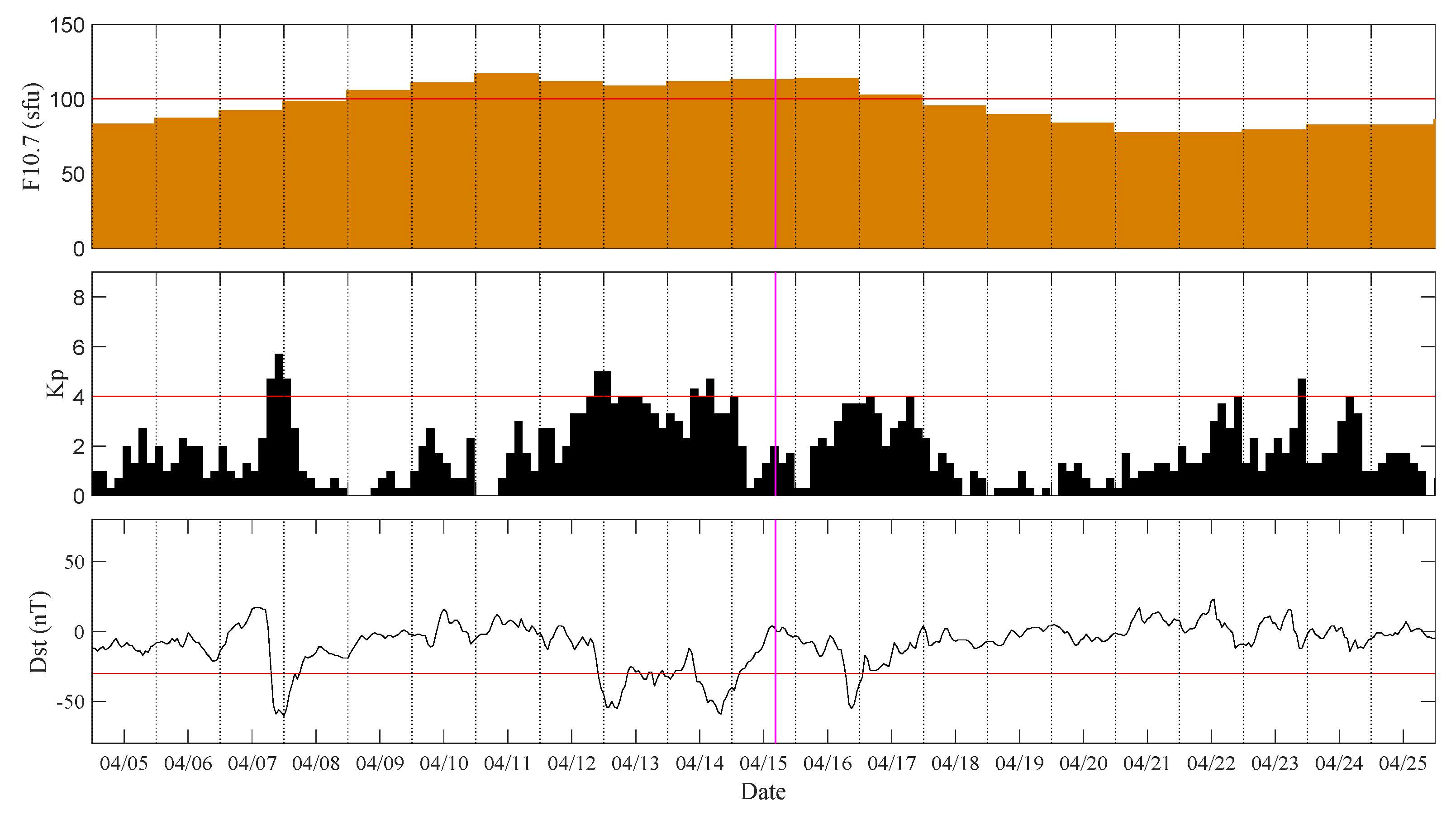
From 8 to 17 April, the solar-geomagnetic conditions were not quiet. It can be seen from Figure 2 that the Kp and Dst index are unstable during this period. On 7, 12, 14, 16 April, a sharp increase appears on the Kp index and the value of Kp even exceeds 4. At the same time, a sharp decrease appears in the Dst index, which means active geomagnetic conditions. In addition, during these 10 days, the solar radiation index F10.7 exceeds 100 SFU.

Figure 2.
Solar–geomagnetic conditions before and after the Mw = 7.0 Kumamoto-shi EQ on 15 April 2016 from Kp, Dst, and F10.7 indices. The time of the EQ is annotated by the magenta dotted line.
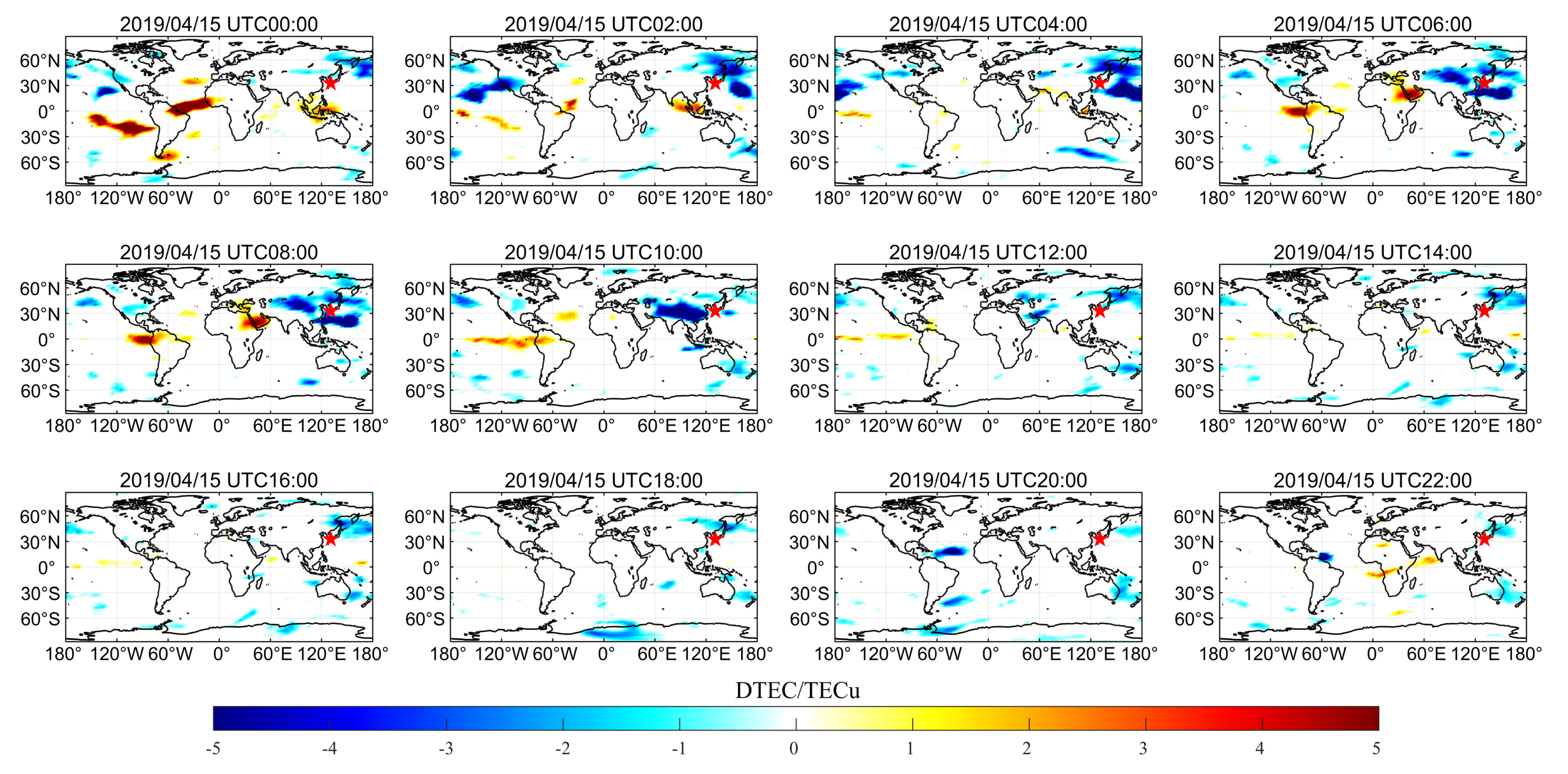
On 15 April 2016, a Mw = 7.0 EQ occurred as a result of strike-slip faulting at shallow depth, with a focal depth of 10 km. As shown in Figure 3, the bihourly GIMs reveal ionospheric anomalies in different locations around the world. At UT = 0 h of the EQ day, significant negative ionospheric anomalies appear over the northeast of the epicenter, which linger until UT = 4 h, and the amplitude of TEC anomaly is about –5 TECu. Then, the anomalous clouds gradually drift southwestward. From UT = 0–8 h, there is a significant positive ionospheric anomaly near the equator, which appears to be more in line with the intensification of Equatorial Ionization Anomaly (EIA). Starting from UT = 12 h, 12 h before the main shock, there are continuous negative ionospheric anomalies lingering in the northeast of the epicenter until UT = 22 h, and the anomaly amplitude is about −3 TECu. The TEC anomalies detected by the correlation analysis before the EQ have some peculiar characteristics. Firstly, the ionospheric anomalies always lingered over or near the epicenter, unlike diurnal changes in the ionosphere or TID, which drift westward at a speed of 100–1000 m/s. According to the statistical analysis of TIDs, the occurrence rate of TID strongly depends on the season and Local Time (LT), and in these regions—dawn (05:00–07:00 LT) and dusk (17:00–20:00 LT) in summer (May–August), and daytime (08:00–12:00 LT) in winter (November–February)—TID has the highest probability of being discovered. [31,32] Secondly, the range and extent of ionospheric anomalies are related to the magnitude of the EQ and the depth of the focal point. The earthquake occurred at 1:25 am (LT) on 15 April (spring), which is not in the high-occurrence period of TID. In addition, the ionospheric cloud over the epicenter that appeared on 15 April did not have the drift characteristics of TID. So, the persistent, slightly negative ionospheric anomaly northwest of the epicenter that lingered from UT = 12–22 h may be related to the impending main shock.

Figure 3.
Bi−hourly GIMs for Mw = 7.0 Kumamoto-shi EQ on 15 April 2016 (main shock day). The red star represents the epicenter location. The UTC is shown as the title on each panel.
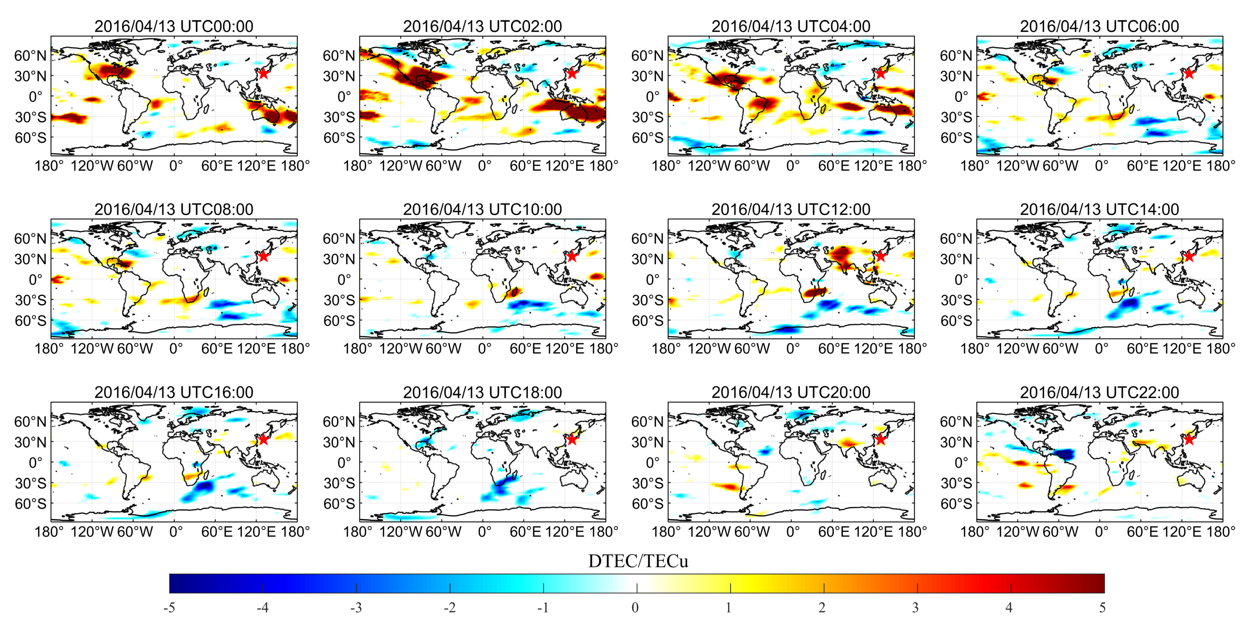
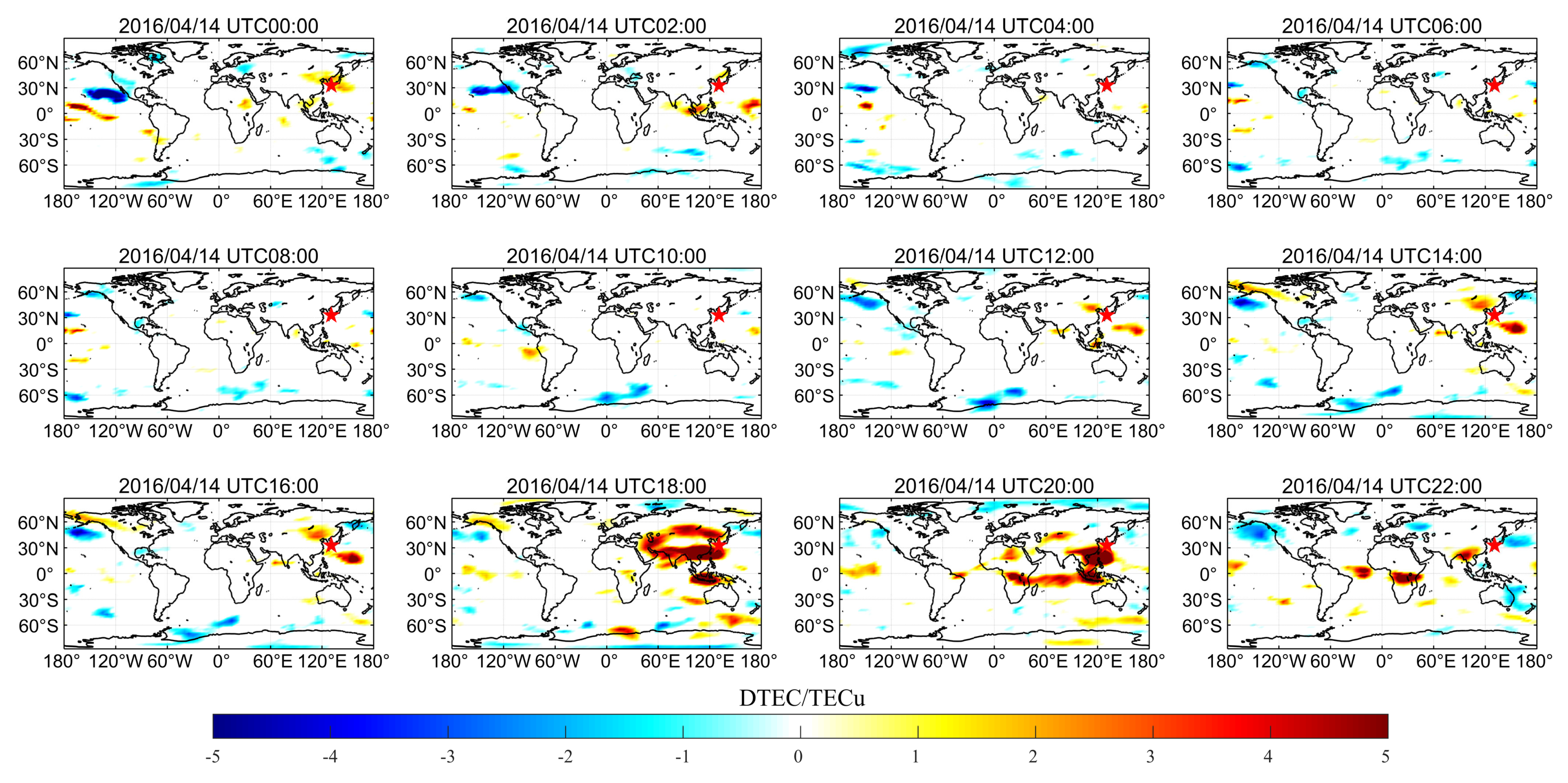
We compared the ionospheric anomalies presented by GIMs on 13–15 April and analyzed the similarities and differences among them to verify that the occurrence of ionospheric anomalies was related to EQ rather than active solar-geomagnetic conditions (Dst < −30 nT, Kp > 4, and F10.7 > 100 SFU) on 15 April. The solar-geomagnetic conditions on 13 April were very similar to the main shock day. As can be seen in Figure 4, from UT = 0–4 h, significant positive ionospheric anomalies appear globally, without spatial distribution characteristics related to the impending main shock. Starting from UT = 6 h, the global ionospheric anomalies begin to fade away. At UT = 12 h, significant positive and negative ionospheric anomalies appear again on both sides of the equator. The positive and negative ionospheric anomalies are distributed globally, and their characteristics are similar to those induced by active solar-geomagnetic conditions. There is a time lag between the ionospheric anomalous response and the solar-geomagnetic conditions, as they are not exactly simultaneous [33]. Referring to Figure 5, a similar phenomenon appears on 14 April. At UT = 0 h, a slightly positive ionospheric anomaly appears near the epicenter and disappears soon after. Starting from UT = 12 h, significant positive ionospheric anomalies begin to appear over the epicenter and drift to the southwest. Suddenly intensified positive ionospheric anomalous clouds of ionosphere appear on both sides of the equator at UT = 18–20 h.

Figure 4.
Bi−hourly GIMs for Mw = 7.0 Kumamoto-shi EQ on 13 April 2016. The red star represents the epicenter location. The UTC is shown as title on each panel.
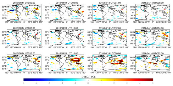
Figure 5.
Bi−hourly GIMs for Mw = 7.0 Kumamoto-shi EQ on 14 April 2016 (main shock day). The red star represents the epicenter location. The UTC is shown as title on each panel.
In general, the ionospheric anomalies caused by active solar-geomagnetic conditions are different in magnitude and scope from the ionospheric anomalies caused by the EQ. Otsuka et al. proposed that the drift trend from northeast to southwest and the shape of ionospheric anomalous clouds are consistent with the previous study of TID over Japan induced by active solar-geomagnetic conditions [34]. The significant positive ionospheric anomalies that appeared on 13–14 April are attributed to active solar-geomagnetic conditions. By comparing Figure 4 and Figure 5 with Figure 3, we can find that the ionospheric anomalies in the GIMs are completely different. As a whole, the anomalous clouds induced by EQ on 15 April stay near the epicenter without drifting. The TEC anomalies before large EQs do not propagate as a circular TID, because the mechanism is radically different from the mechanism of TIDs [18].
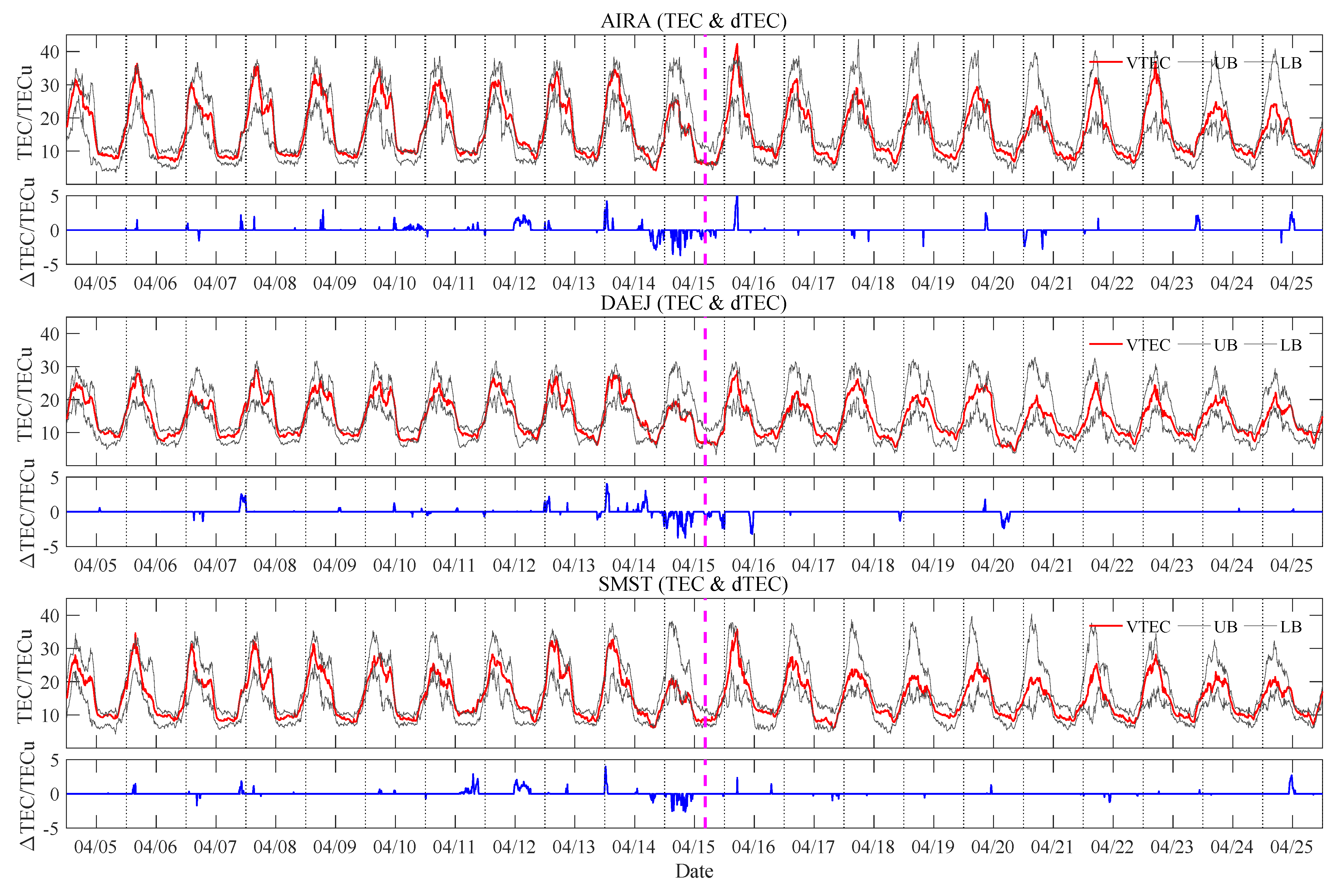
In order to further explore the preseismic anomaly of the ionosphere, the ionospheric anomalies were studied by 10 min-sampling-interval VTEC from three GPS stations. The VTEC time-series and its associated lower and upper bounds are shown in Figure 6. It can be seen that intermittent ionospheric TEC enhancement and depletion are observed. The pre-ionospheric enhancement on 14 April, reaching 5 TECu, is more likely to be caused by the active solar-geomagnetic conditions. This is consistent with the phenomena presented in the GIMs (Figure 5), which provide evidence to justify our statistical bounds manifestation. The earliest negative ionospheric anomaly appeared 8 days before the EQ, observed by three GPS stations. Only from two days before the EQ to the EQ day, there was a prominent eruption of negative ionospheric anomalies, reaching −3 TECu. Especially, on 15 April 2016—the main shock day—significant ionospheric negative anomalies were observed by three GPS stations. After the EQ, intermittent positive and negative ionospheric anomalies were also discovered.
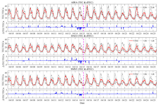
Figure 6.
Temporal VTEC from three GPS ground−stations for analysis of anomalous values before and after the Mw = 7.0 Kumamoto-shi EQ on 15 April 2016. The time of the EQ is annotated by the magenta dotted line (see Table 1 for EQ details). The upper bound (UB) and lower bound (LB) are shown in gray, and TEC is shown in red. The blue curve represents .
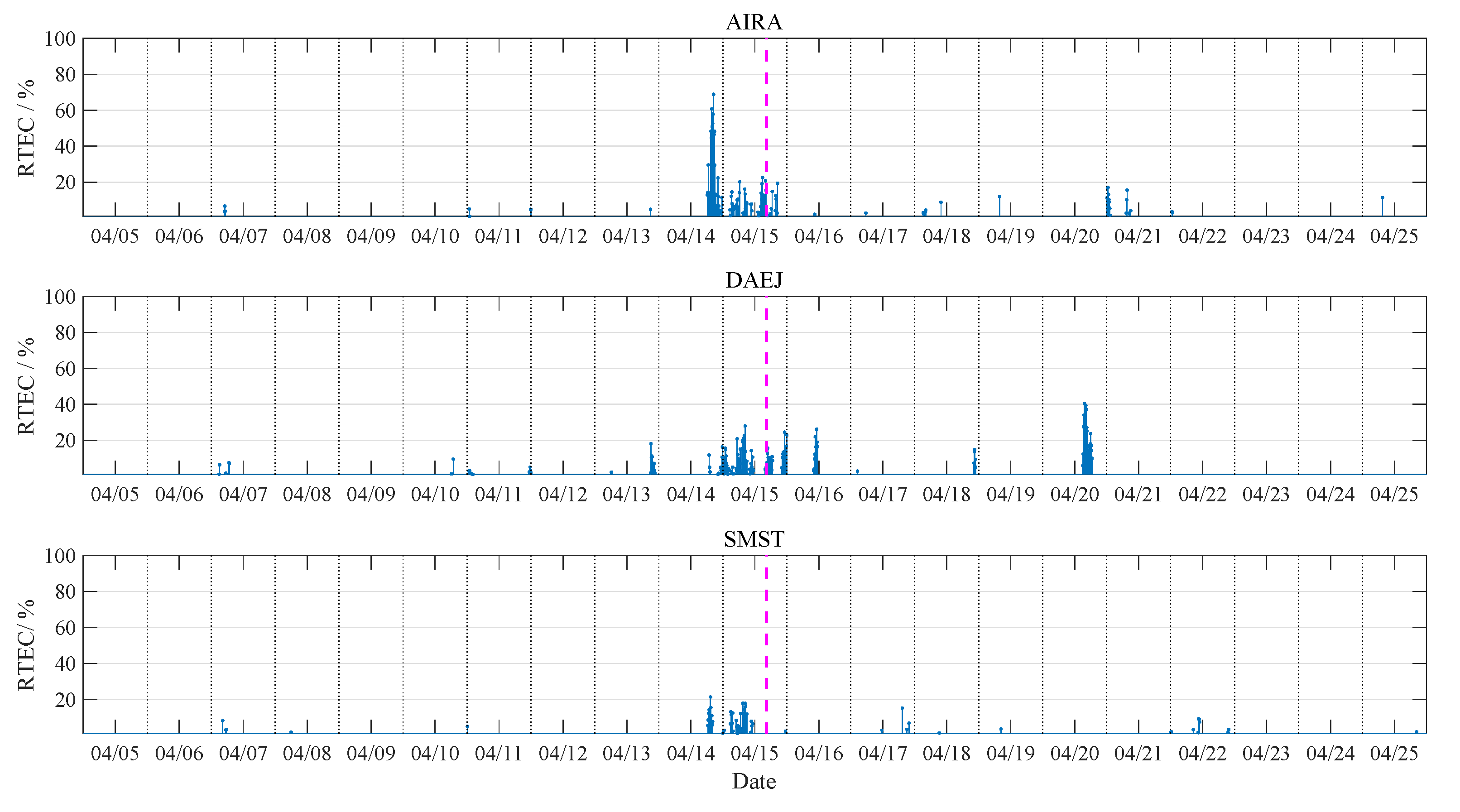
Moreover, the extent of relative negative ionospheric anomalies calculated by Equation (6) are shown in Figure 7. It is found that the negative ionospheric anomalies are particularly obvious on the day of the EQ. The abnormal ionospheric TEC depletions before the EQ are likely to be caused by the process of EQ incubation. This phenomenon is consistent with Figure 6 and Figure 7, showing that significant negative ionospheric anomalies were detected on 15 April (earthquake day), including GIMs and VTEC from GPS stations.
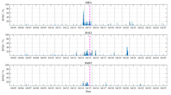
Figure 7.
Relative TEC for Mw = 7.0 Kumamoto-shi EQ on 15 April 2016 from three stations and analysis of 10 days before and after the main shock (only negative ionospheric anomalies are shown in stem). The time of the EQ is annotated by the magenta dotted line.
3.2. Jinghe, China Earthquake
Variations in the solar-geomagnetic conditions are obstacles to accurately identify ionospheric anomalies before EQs. We selected the EQ that occurred on 8 August 2017 in Jinghe, China as the research object under quiet solar-geomagnetic conditions (Dst > −30 nT, Kp < 4, and F10.7 < 100 SFU), as shown in Figure 8.
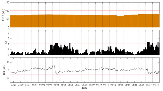
Figure 8.
Solar–geomagnetic conditions before and after Mw = 6.3 Jinghe EQ on 8 August 2017 from Kp, Dst, and F10.7 indices. The time of the EQ is annotated by the magenta dotted line.
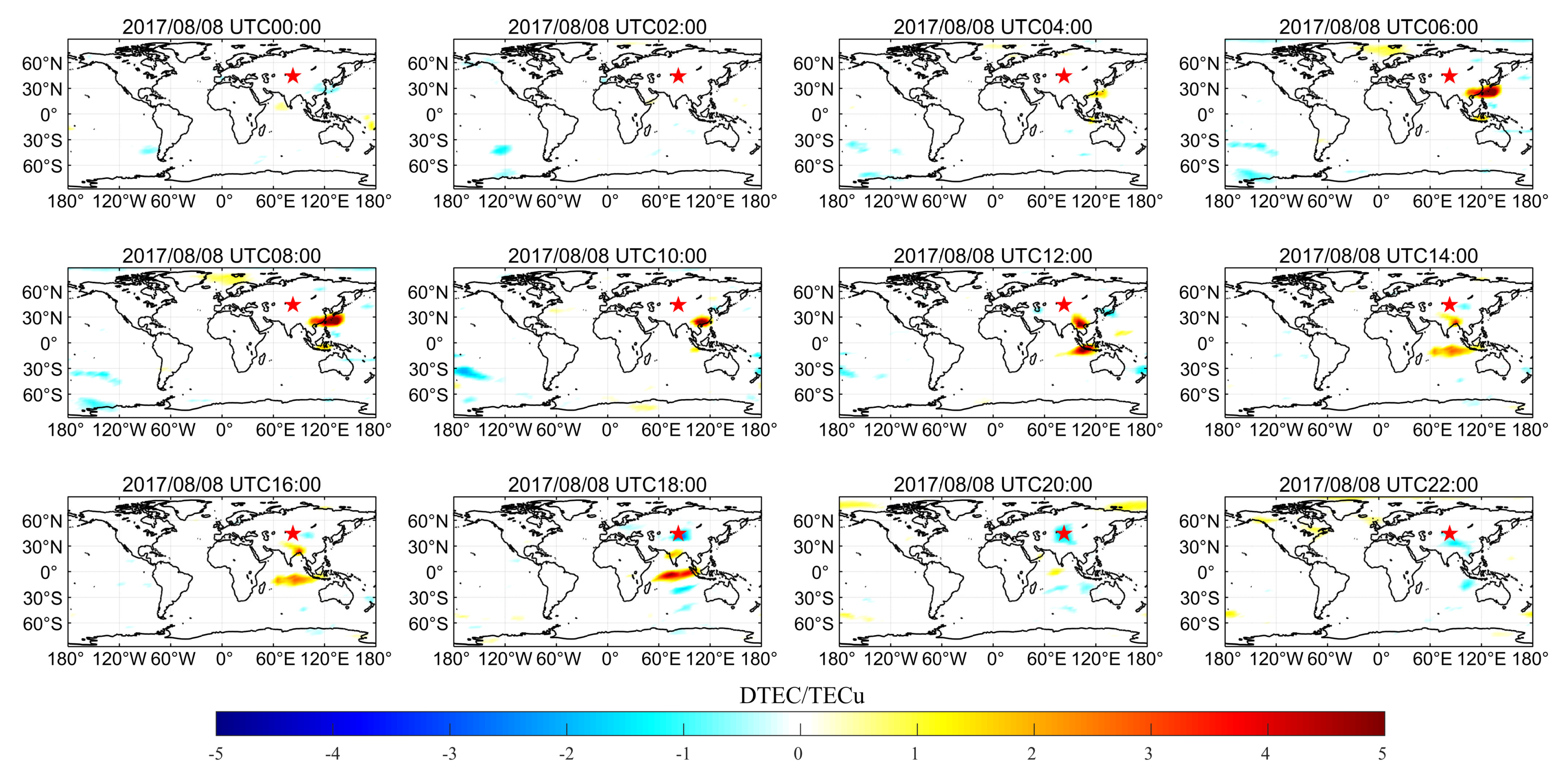
The epicenter is far from the ocean and at a higher latitude than the Kumamoto-shi EQ; so, the ionosphere above the epicenter is not easily affected by the EIA. The bihourly GIMs (Figure 9) show that at UT = 4 h, a slightly positive ionospheric anomaly appears close to the equator. The abnormal value gradually increases, reaching a peak of 5 TECu at UT = 6 h and drifting westward. At UT = 12 h, a positive conjugate ionospheric anomaly appears on the south side of the equator. The characteristics of such anomalies are consistent with the TID. At the same time, 9 h before the EQ, a slightly negative ionospheric anomaly begins to appear near the epicenter and far from the equator. At UT = 14 h, it hits a peak, which is lower than −3 TECu. These negative ionospheric anomalous clouds linger until UT = 20 h, 3 h before the EQ. There is no significant drift and the clouds remain above the epicenter. We investigated the solar-geomagnetic conditions when the EQ occurred, and attributed these anomalous clouds of TEC to the impending main shock under quiet solar-geomagnetic conditions, as it is different with characteristics of two-crest equatorial region.

Figure 9.
Bi−hourly GIMs for Mw = 6.3 Jinghe EQ on 8 August 2017 (main shock day). The red star represents the epicenter location. The UTC is shown as the title on each panel.
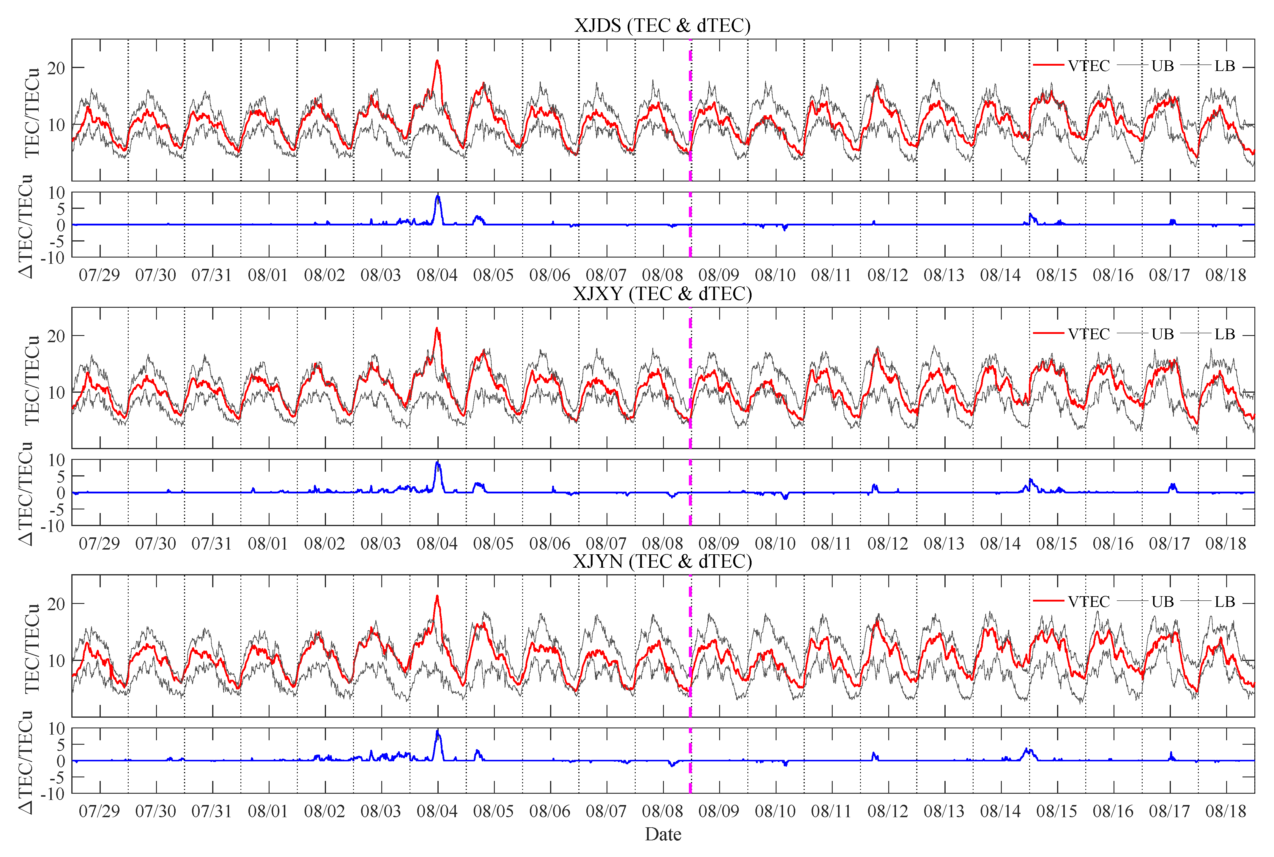
The temporal series of GPS TEC extracted from three permanent GPS stations is shown in Figure 10. It can be found that the slightly negative ionospheric anomalies first appear on 29 July, 10 days before the EQ. Then, from two days before to the day of the EQ, significant negative ionospheric anomalies are observed by three GPS stations, with amplitudes of −2 TECu. On 10 August, two days after the EQ, the negative ionospheric anomaly appears again. What cannot be ignored is that during 3–5 August, positive ionospheric anomalies erupt intensely, especially peaking with 10 TECu on 4 August, 4 days before the main shock. We can see from Figure 8 that the Kp exceeds 4 on 4 and 6 August, and the Dst shows a positive sudden change, then drops sharply on 4 August. Therefore, the positive ionospheric anomalies during these days are mainly related to active geomagnetic activities (Kp > 4, Dst < −30 nT). It further proves that ionospheric TEC will respond to active geomagnetic conditions. In the case of quiet solar-geomagnetic conditions, the occurrence of these negative ionospheric anomalies are mainly related to the main shock.
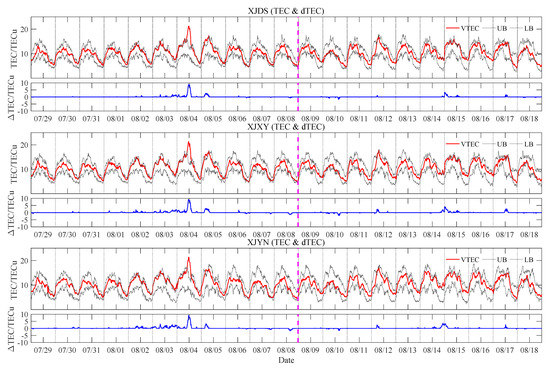
Figure 10.
Temporal VTEC from three GPS ground−stations for analysis of anomalous values before and after Mw = 6.3 Jinghe EQ on 8 August 2017. The time of the EQ is annotated by the magenta dotted line (see Table 1 for EQ details). The upper bound (UB) and lower bound (LB) are shown in gray, and TEC is shown in red. The blue curve represents .
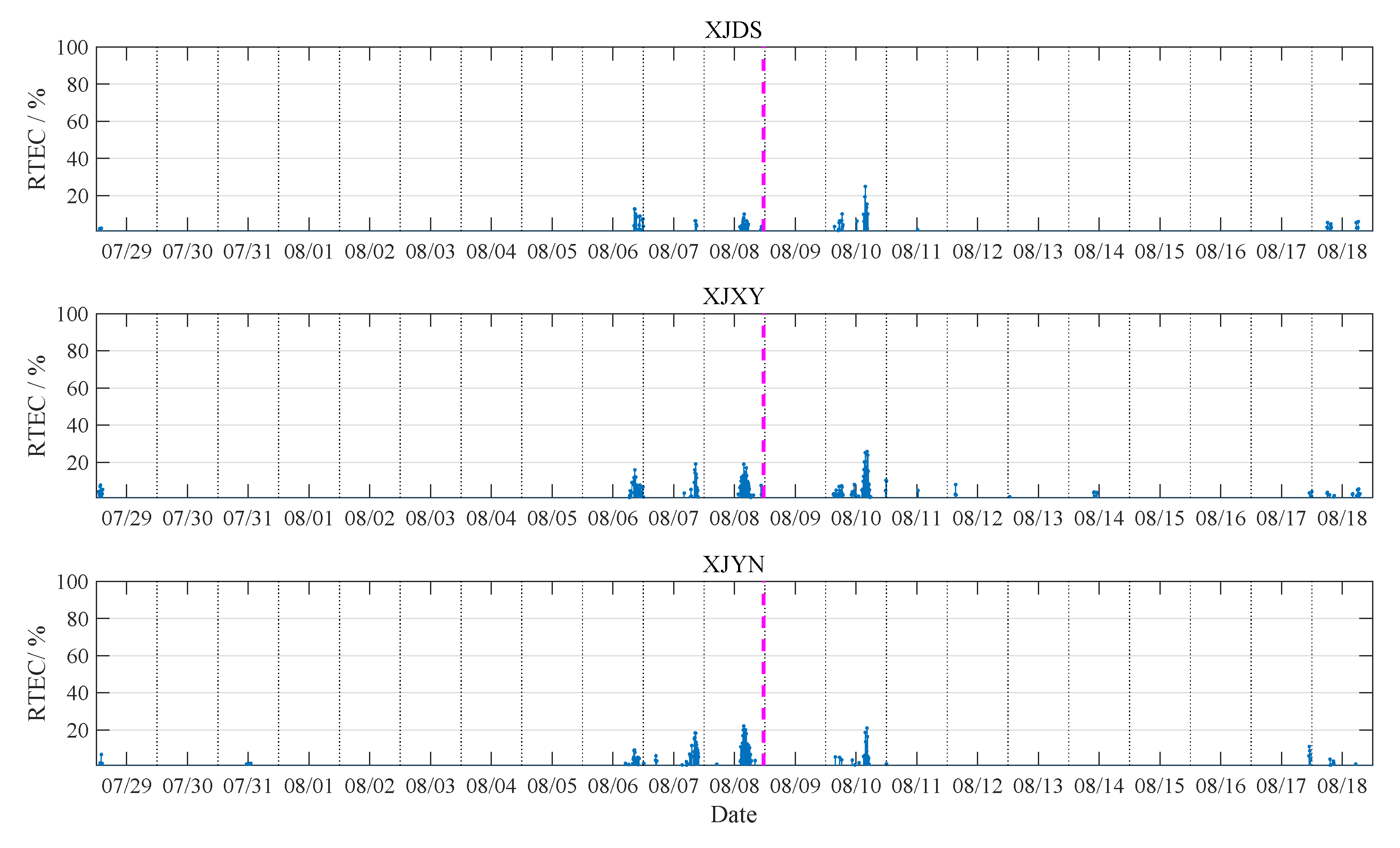
Similarly, we studied the RTEC of Jinghe EQ. It can be seen from Figure 11 that 3 days before and 2 days after the EQ, the negative ionospheric anomalies observed by three GPS stations are prominent, with RTEC exceeding 20%. According to the above analyses, the phenomena presented in Figure 9, Figure 10 and Figure 11 are consistent, showing that negative ionospheric anomalies appear above the epicenter on the EQ day. Under quiet solar-geomagnetic conditions, the negative ionospheric anomalies during 2 days before to 2 days after the main shock may be caused by the EQ.
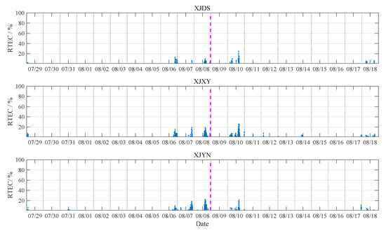
Figure 11.
Relative TEC for Mw = 6.3 Jinghe EQ on 8 August 2017 from three stations, and analysis of 10 days before and after the main shock (only negative ionospheric anomalies are shown in stem). The time of the EQ is annotated by the magenta dotted line.
3.3. Lagunas, Peru Earthquake
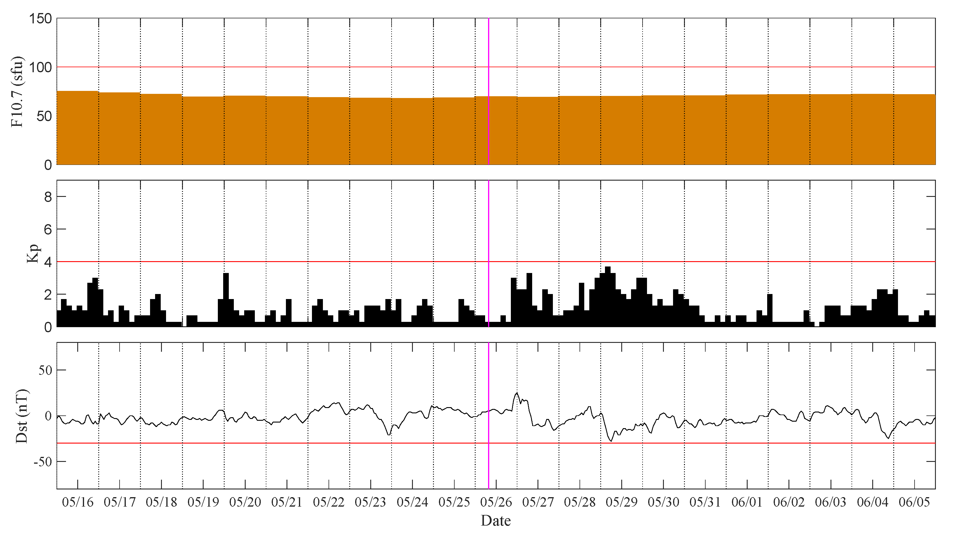
The previous two cases show that negative ionospheric anomalies are found near the epicenter on EQ-related days and the extent of ionospheric anomalies caused by EQs is different. However, there are no exact characteristics about seismo-ionospheric anomalies. Shah and Jin [10] claimed that GPS TEC anomalies depend on the magnitude and hypocentral depth of future EQs and can also be attributed to different fault systems. We selected the Lagunas, Peru EQ that occurred on 26 May 2019 with Mw = 8.0 for research, which is the result of normal faulting at an intermediate depth, approximately 110 km beneath the Earth’s surface. During the EQ breed period, the Solar-geomagnetic conditions are quiet, with Kp < 4, −30 nT < Dst < 30 nT, and F10.7 < 100 SFU, as shown in Figure 12.

Figure 12.
Solar–geomagnetic conditions before and after Mw = 8.0 Peru on 26 May 2019 from Kp, Dst, and F10.7 indices. The time of the EQ is annotated by the magenta dotted line.
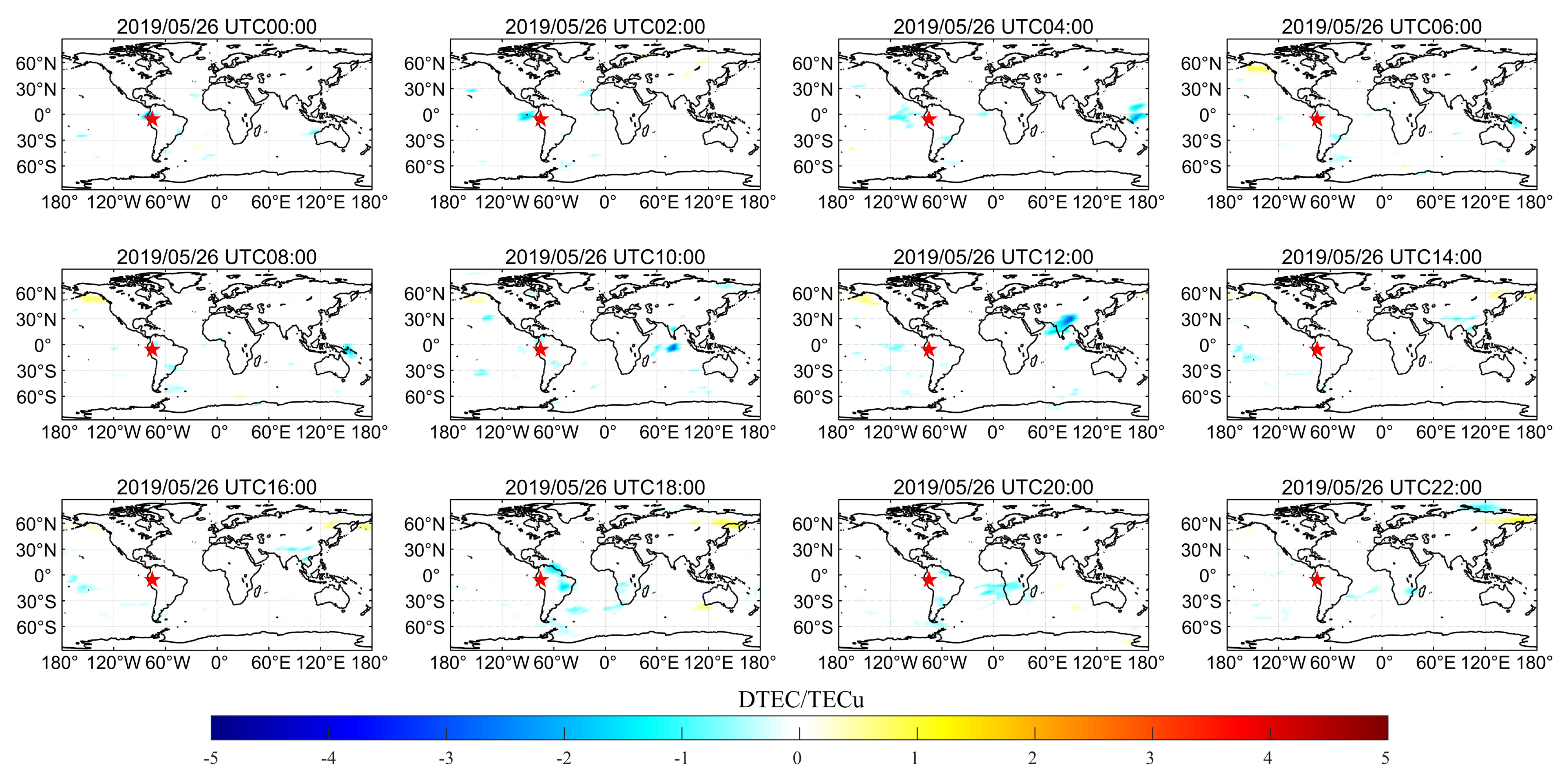
Similarly, we analyzed the temporal and spatial distribution of ionospheric anomalies in the GIMs. As can be seen from Figure 13, at UT = 0 h, a slightly negative ionospheric anomaly appears above the epicenter and the peak value is −3 TECu; then, the anomalous clouds gradually drift westward. At UT = 6 h, a slightly negative ionospheric anomaly appears again over the north of the epicenter. Until UT = 10 h, after the main shock occurs, the slightly negative ionospheric anomaly begins to fade. The range and extent of negative ionospheric anomalies are small, which may be related to the deep focal depth of the EQ. At UT = 12 h, significant conjugate negative ionospheric anomalies appear on both sides of the equator and drift from east to west. The slightly negative ionospheric anomalous clouds at UT = 0–10 h may be caused by the process of EQ incubation, according to the characteristics of the seismo-ionospheric anomaly.
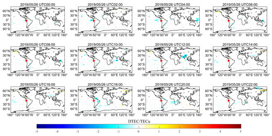
Figure 13.
Bi−hourly GIMs for Mw = 8.0 Peru on 26 May 2019 (main shock day). The red star represents the epicenter location. The UTC is shown as the title on each panel.
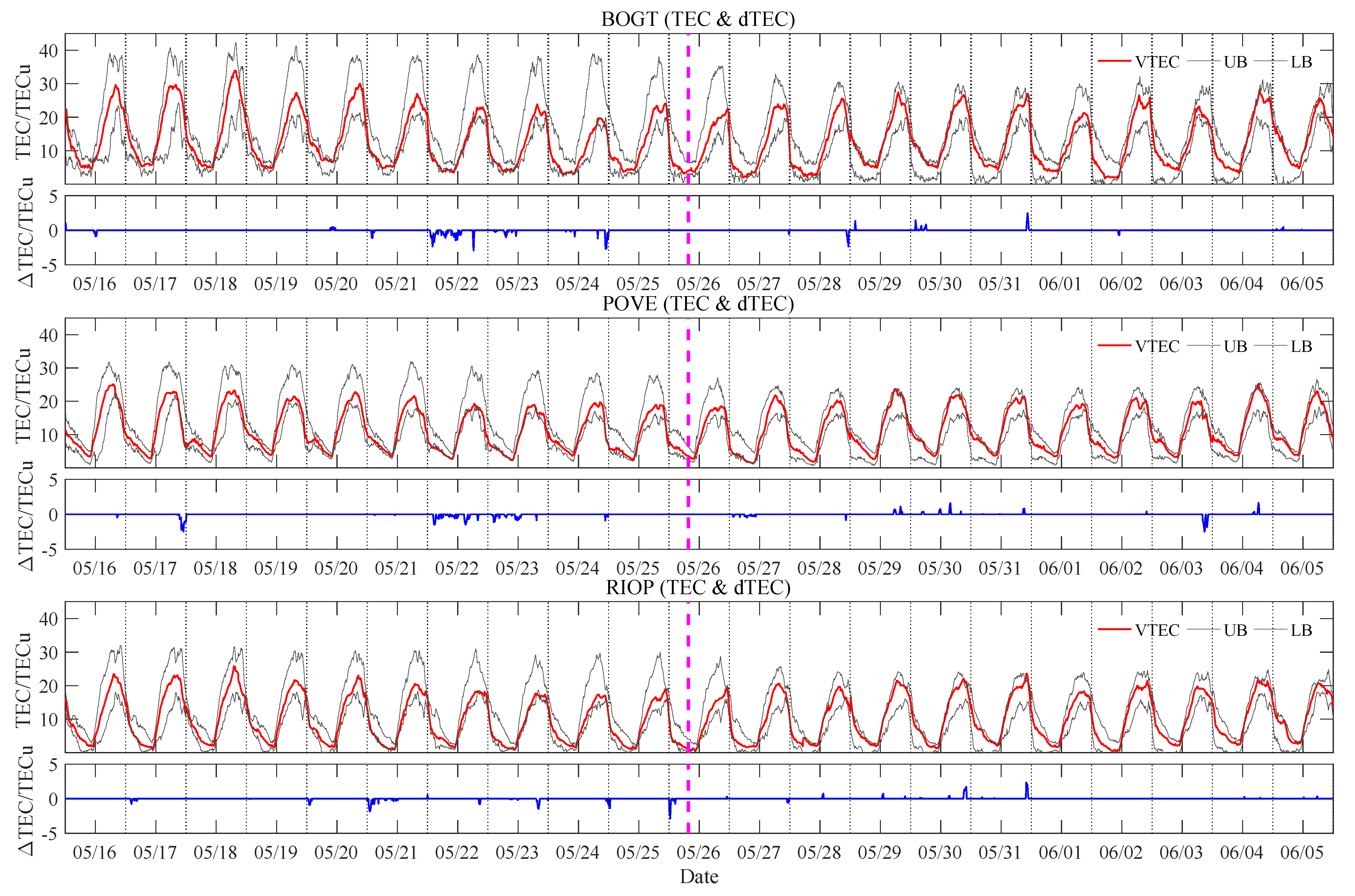
The TEC data from 3 GPS stations near the epicenter were extracted for research. It can be seen from Figure 14 that as early as 10 days before the EQ, slightly negative ionospheric anomalies were observed by the BOGT station. From 5 days before the EQ to the day of the main shock, the negative ionospheric anomalies begins to appear frequently, and the amplitude reaches −3 TECu. During the 10 days after the EQ, negative ionospheric anomalies appear occasionally, not as significantly as before the EQ. During the earthquake incubation period, the ionosphere could be continuously affected by the energy released from epicenter, resulting in changes in the scale of the negative ionospheric anomaly. No significant positive ionospheric anomalies were found by three GPS stations in these 21 days under quiet solar-geomagnetic conditions (Dst > −30 nT, Kp < 4, and F10.7 < 100 SFU).
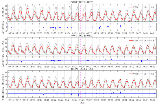
Figure 14.
Temporal VTEC from three GPS ground−stations for analysis of anomalous values before and after Mw = 8.0 Peru on 26 May 2019. The time of the EQ is annotated by the magenta dotted line (see Table 1 for EQ details). The upper bound (UB) and lower bound (LB) are shown in gray, and TEC is shown in red. The blue curve represents .
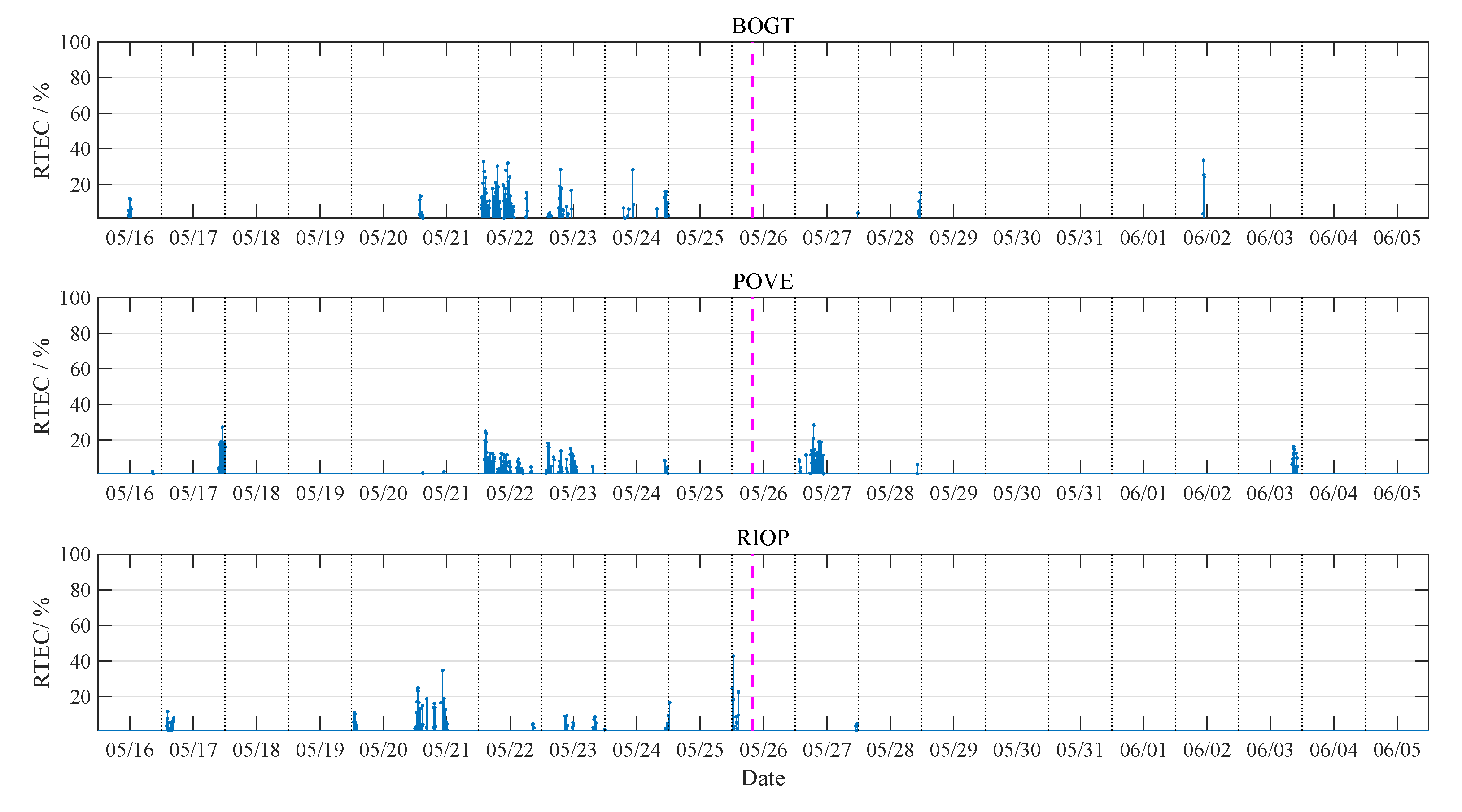
We studied the RTEC of this EQ. As shown in Figure 15, the statistical results of the three stations show that from 5 days before the EQ to the day of the EQ, significant negative ionospheric anomalies are observed. The negative ionospheric anomalies before the EQ show some temporal correlation with the main shock. Therefore, we believe that the ionospheric anomalies above the epicenter are caused by EQ.
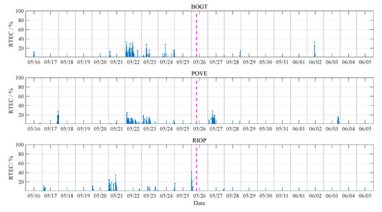
Figure 15.
Relative TEC for Mw = 8.0 Peru on 26 May 2019 from three stations, and analysis of 10 days before and after the main shock (only negative ionospheric anomalies are shown in stem). The time of the EQ is annotated by the magenta dotted line.
In the analysis of these three cases, we found that negative ionospheric anomalous clouds appeared 4–8 h before the main shock and lingered for 4–10 h. During the 21 EQ-related days, negative ionospheric anomalies were observed as early as 10 days before the EQ and as late as 8 days after the EQ. The specific pre/post-TEC precursor information is shown in Table 2.
Table 2.
Associated pre/post-TEC precursors observed by GPS stations (the negative sign represents the number of days before the EQ, and the positive sign represents the number of days after the EQ).
4. Discussion
Ionospheric anomalies related to three major Mw > 6.0 EQs were analyzed in this paper. In the bihourly GIMs, we found that before the main shock, there are significant negative ionospheric anomalies over or near the epicenter, which is different from ionospheric anomalies caused by active solar-geomagnetic conditions or TID. For each EQ, during the 21 EQ-related days, we discovered some negative ionospheric anomalies related to the process of EQ incubation. Through the study of the RTEC of the three cases, a common phenomenon is found that the negative ionospheric anomalies during 5 days before to 2 days after the EQs are more prominent than the other days, under various solar-geomagnetic conditions. There are some similarities with the research results proposed by Pulinets and Davidenko [18] on the temporal characteristics of seismo-ionospheric anomalies.
In case of the Kumamoto’s Mw = 7.0 EQ, which occurred on 15 April 2016, active solar-geomagnetic conditions are recorded from 8–17 April. In previous researches, the active solar-geomagnetic conditions and EQ are both considered to be main causes of ionospheric anomalies [35]. Although not all geomagnetic activities can cause anomalies in the ionosphere [4], it is difficult to conclude that the ionospheric anomalies above the Kumamoto-shi on 15 April are induced by the upcoming EQ. We analyzed the ionospheric anomalies on 13–14 April, under almost the same active solar-geomagnetic conditions (Dst < −30 nT, Kp > 4, and F10.7 > 100 SFU). It is found that a wide range of positive ionospheric anomalies appear near the equator in these two days and the characteristics of anomalous clouds are very consistent with the mesoscale ionospheric anomalies caused by active geomagnetic conditions. The shape and drift trend of ionospheric anomalies over the epicenter on 15 April is significantly different. Furthermore, only the significant negative ionospheric anomalies on 15 April were observed by three permanent GPS stations during 21 EQ-related days. Therefore, the negative ionospheric anomalies on this day were mainly caused by the EQ. Iwata and Umeno [31] proposed the same conclusion by studying the characteristics of abnormal ionospheric cloud drift over Japan.
For the Jinghe EQ, ionospheric TEC responds to variations in solar-geomagnetic conditions differently. It is found that on the day of the EQ, there was a significant negative ionospheric anomaly over the epicenter, under quiet solar-geomagnetic conditions (Dst > −30 nT, Kp < 4, and F10.7 < 100 SFU). The ionospheric TEC responding to active solar-geomagnetic conditions further prove that under quiet conditions, EQ is the cause of negative ionospheric anomalies. Under absolutely quiet solar-geomagnetic conditions, similar temporal distribution of negative ionospheric anomalies were also found in the Lagunas EQ. However, the ionospheric negative anomalies are so weak that they cannot remain above the epicenter for a long time due to the fact that energy released by the seismic fault zone needs to travel a long distance to reach the surface.
In order to further explain how EQs cause ionospheric anomalies, some studies have explained them from the perspective of physics. Friedemann and Freund [2] proposed that the collision between rocks generates high-speed charge carriers, which form a fluctuating charge cloud; this can explain the electrical signals and electromagnetic radiation associated with EQs. Similarly, the investigation of temporal and spatial measurements suggested that abrupt anomalies observed within 10 days before the 2007 Mw = 7.7 Chile EQ were considered to be the fragments of the plasma intensification process in the southern hemisphere activated by the rock compression in the quake region [36]. Kuo et al. [20] proposed a coupling model for the stressed-rock–Earth surface-charge–atmosphere system. The stressed-rock acts as the dynamo to provide the currents for the coupling system. The current in the EQ fault zone has an impact on the electric fields and currents in the atmosphere and the lower boundary of ionosphere as well as the formation of a plasma bubble. The constant current flow from the EQs epicenter can further stimulate the horizontal electric field at the bottom of the ionosphere to initiate the vertical or zonal drift of ionospheric plasma following the magnetic field direction. On the other hand, Pulinets et al. [12] demonstrated that the observed variations of the atmosphere and ionosphere parameters have a common cause—the air ionization by radon. A significant depletion in ionospheric TEC was observed in the month of earthquake occurrence by performing long-term statistics. This is consistent with the findings of this paper.
The coupling mechanism between the EQ and ionosphere is very complex and difficult to measure. It still needs more observation by ionospheric measurements from GPS and other techniques. In other studies, the observations of different ionospheric parameters is available; for example, the variation in foF2, observed by the ionosonde, has a similar tendency and is highly correlated with overhead TEC recorded by GPS before EQ. Namely, within 1–5 days before the EQ, significant depletions on foF2 and TEC were observed [11]. This has some similarities with the results of this paper. The electron temperature measurements from Langmuir Probe (ISL) of Detection of Electromagnetic Emissions Transmitted from EQ Region (DEMETER) can also be used as an indicator to judge the ionospheric anomalies. The disturbances in the electron density observed by CHAMP satellite and the concurrent electric field and Ne changes suggest that EIA intensification could be triggered by the E field disturbances over the epicenter [37]. In terms of ionospheric TEC, the ambiguity-fixed carrier-phase ionospheric observable is more accurate than the carrier-phase leveled-code one [38]. The distribution and changes of electrons in the ionosphere can be observed by ionospheric tomography method in more detail [39].
5. Conclusions
In this paper, the seismo-ionospheric TEC anomalies associated with three Mw > 6.0 EQs were detected by GIMs and GPS-TEC. We analyzed the spatial and temporal variations of the ionospheric TEC under various solar-geomagnetic conditions. The main findings of this research are as follows:
- The negative ionospheric anomalies observed within 10 days before the main shock could be considered significant signals of upcoming EQs. In the analysis of the three EQ cases, we found significant negative ionospheric anomalies with TEC reaching −3 TECu before the main shock. On the day of Jinghe EQ and Lagunas EQ, the negative ionospheric anomaly clouds linger over or near the epicenter for 4–10 h, under quiet solar-geomagnetic conditions (Kp < 4, Dst > −30 nT, and F10.7 < 100 SFU). In the case study of the Kumamoto-shi, Japan EQ, on the day of the EQ, the negative ionospheric anomalies are observed under active solar-geomagnetic conditions and are significantly different from those caused by the same solar-geomagnetic conditions.
- The negative ionospheric anomalies are more prominent during 5 days before to 2 days after the EQ than the other days. In the analysis of three EQ cases, negative ionospheric anomalies were found with RTEC exceeding 20% during this period. These ionospheric anomalies manifest a significant temporal correlation with the main shock.
- Ionospheric TEC responds differently to various solar-geomagnetic conditions. In the case study of Kumamoto-shi, Japan EQ, abnormal ionospheric TEC enhancement appears under active solar-geomagnetic conditions (Kp > 4, Dst < −30 nT, and F10.7 > 100 SFU) 2 days before the main shock and the abnormal amplitude reaches 5 TECu. Similar TEC variations also appear in the research of Jinghe EQ on the 4th day before the main shock with amplitude reaching 10 TECu, under active geomagnetic conditions (Kp > 4 and Dst < −30 nT). On 15 April 2016 and 17–18 August 2017, the ionospheric TEC enhancement did not occur, even though the solar-geomagnetic conditions are still active.
Finally, we discussed the other parameters that reflect the characteristics of the ionosphere and the merging process of seismo-ionospheric TEC anomalies. More detailed studies need to be performed to distinguish the ionospheric anomalies caused by EQs.
Author Contributions
Conceptualization, Y.D. and C.G.; methodology, Y.D. and F.L.; software, Y.D.; validation, Y.D. and Y.Y.; formal analysis, Y.D. and F.L.; investigation, Y.D. and F.L.; resources, Y.D. and C.G.; data curation, Y.D. and Y.Y.; writing—original draft preparation, Y.D.; writing—review and editing, Y.D., C.G. and F.L.; visualization, Y.D. and Y.Y; supervision, C.G. and F.L.; project administration, Y.D. and C.G.; funding acquisition, C.G. and F.L. All authors have read and agreed to the published version of the manuscript.
Funding
Postgraduate Research & Practice Innovation Program of Jiangsu Province: KYCX17_0150; Hebei Xiongan Jingde Expressway Co., Ltd.: JD-202011.
Institutional Review Board Statement
Not applicable.
Informed Consent Statement
Not applicable.
Data Availability Statement
The detailed information of EQs was retrieved from U.S. Geological Survey (USGS): http://www.earthquake.usgs.gov/earthquakes/search (accessed on 5 November 2021). Dst and Kp indices were obtained from the International Service of Geomagnetic Indices (ISGI): http://isgi.unistra.fr (accessed on 5 November 2021). The solar radiation index F10.7 obtained from the Space Physics Data Facility (SPDF): https://omniweb.gsfc.nasa.gov/form/dx1.html (accessed on 5 November 2021). The global ionospheric maps (GIMs) were acquired from the Center for Orbit Determination in Europe (CODE): http://ftp.aiub.unibe.ch/CODE/ (accessed on 5 November 2021). RINEX data of permanent GPS observatories in China (XJDS, XJXY, XJYN) were obtained from the Crustal Movement Observation Network of China (CMONOC). The rest (AIRA, DAEJ, SMST, BOGT, POVE, RIOP) were obtained from International GNSS services (IGS) observatories: http://www.igs.gnsswhu.cn/index.php/Home/DataProduct/igs.html (accessed on on 5 November 2021).
Acknowledgments
The authors are very grateful to the U.S. Geological Survey, International Service of Geomagnetic Indices, and Space Physics Data Facility for providing EQs and solar-geomagnetic conditions data. We are also thankful to International GNSS Service, Center for Orbit Determination in Europe, and Crustal Movement Observation Network of China for GIMs and TEC of permanent GPS ground-stations. We are also thankful to the Editor-in-Chief, Associate Editor.
Conflicts of Interest
The authors declare no conflict of interest.
References
- Leonard, R.S.; Barnes, R.A. Observation of ionospheric disturbances following the Alaska earthquake. J. Geophys. Res. 1965, 70, 1250–1253. [Google Scholar] [CrossRef]
- Freund, F. Time-resolved study of charge generation and propagation in igneous rocks. J. Geophys. Res. Solid Earth 2000, 105, 11001–11019. [Google Scholar] [CrossRef] [Green Version]
- Liu, J.Y.; Chen, Y.I.; Pulinets, S.A.; Tsai, Y.B.; Chuo, Y.J. Seismo-ionospheric signatures prior to M ≥ 6.0 Taiwan earthquakes. Geophys. Res. Lett. 2000, 27, 3113–3116. [Google Scholar] [CrossRef]
- Burešová, D.; Laštovička, J. Pre-storm enhancements of foF2 above Europe. Adv. Space Res. 2007, 39, 1298–1303. [Google Scholar] [CrossRef]
- Ahmed, J.; Shah, M.; Zafar, W.A.; Amin, M.A.; Iqbal, T. Seismoionospheric anomalies associated with earthquakes from the analysis of the ionosonde data. J. Atmos.-Sol.-Terr. Phys. 2018, 179, 450–458. [Google Scholar] [CrossRef]
- Ciraolo, L.; Azpilicueta, F.; Brunini, C.; Meza, A.; Radicella, S.M. Calibration errors on experimental slant total electron content (TEC) determined with GPS. J. Geod. 2007, 81, 111–120. [Google Scholar] [CrossRef]
- Liu, J.Y.; Chen, Y.I.; Chuo, Y.J.; Chen, C.S. A statistical investigation of preearthquake ionospheric anomaly. J. Geophys. Res. 2006, 111, A05304. [Google Scholar] [CrossRef] [Green Version]
- Shah, M.; Inyurt, S.; Ehsan, M.; Ahmed, A.; Shakir, M.; Ullah, S.; Iqbal, M.S. Seismo ionospheric anomalies in Turkey associated with M ≥ 6.0 earthquakes detected by GPS stations and GIM TEC. Adv. Space Res. 2020, 65, 2540–2550. [Google Scholar] [CrossRef]
- Guo, J.; Li, W.; Yu, H.; Liu, Z.; Zhao, C.; Kong, Q. Impending ionospheric anomaly preceding the Iquique Mw8.2 earthquake in Chile on 2014 April 1. Geophys. J. Int. 2015, 203, 1461–1470. [Google Scholar] [CrossRef]
- Shah, M.; Jin, S. Statistical characteristics of seismo-ionospheric GPS TEC disturbances prior to global Mw ≥ 5.0 earthquakes (1998–2014). J. Geodyn. 2015, 92, 42–49. [Google Scholar] [CrossRef]
- Liu, J.Y.; Chen, Y.I.; Chuo, Y.J.; Tsai, H.F. Variations of ionospheric total electron content during the Chi-Chi Earthquake. Geophys. Res. Lett. 2001, 28, 1383–1386. [Google Scholar] [CrossRef] [Green Version]
- Pulinets, S.A.; Ouzounov, D.; Ciraolo, L.; Singh, R.; Cervone, G.; Leyva, A.; Dunajecka, M.; Karelin, A.V.; Boyarchuk, K.A.; Kotsarenko, A. Thermal, atmospheric and ionospheric anomalies around the time of the Colima M7.8 earthquake of 21 January 2003. Ann. Geophys. 2006, 24, 835–849. [Google Scholar] [CrossRef] [Green Version]
- Saroso, S.; Liu, J.Y.; Hattori, K.; Chen, C.H. Ionospheric GPS TEC Anomalies and M ≥ 5.9 Earthquakes in Indonesia during 1993–2002. Terr. Atmos. Ocean. Sci. 2008, 19, 481. [Google Scholar] [CrossRef] [Green Version]
- Yang, S.S.; Potirakis, S.M.; Sasmal, S.; Hayakawa, M. Natural Time Analysis of Global Navigation Satellite System Surface Deformation: The Case of the 2016 Kumamoto Earthquakes. Entropy 2020, 22, 674. [Google Scholar] [CrossRef] [PubMed]
- Dautermann, T.; Calais, E.; Haase, J.; Garrison, J. Investigation of ionospheric electron content variations before earthquakes in southern California, 2003–2004. J. Geophys. Res. 2007, 112, B02106. [Google Scholar] [CrossRef]
- Thomas, J.N.; Huard, J.; Masci, F. A statistical study of global ionospheric map total electron content changes prior to occurrences of M ≥ 6.0 earthquakes during 2000–2014. J. Geophys. Res. Space Phys. 2017, 122, 2151–2161. [Google Scholar] [CrossRef]
- Afraimovich, E.L.; Astafyeva, E.I. TEC anomalies—Local TEC changes prior to earthquakes or TEC response to solar and geomagnetic activity changes? Earth Planets Space 2008, 60, 961–966. [Google Scholar] [CrossRef] [Green Version]
- Pulinets, S.; Davidenko, D. Ionospheric precursors of earthquakes and Global Electric Circuit. Adv. Space Res. 2014, 53, 709–723. [Google Scholar] [CrossRef]
- Freund, F.T.; Kulahci, I.G.; Cyr, G.; Ling, J.; Winnick, M.; Tregloan-Reed, J.; Freund, M.M. Air ionization at rock surfaces and pre-earthquake signals. J. Atmos. Sol.-Terr. Phys. 2009, 71, 1824–1834. [Google Scholar] [CrossRef]
- Kuo, C.L.; Huba, J.D.; Joyce, G.; Lee, L.C. Ionosphere plasma bubbles and density variations induced by pre-earthquake rock currents and associated surface charges: PRE-EARTHQUAKE IONOSPHERIC EFFECT. J. Geophys. Res. Space Phys. 2011, 116. [Google Scholar] [CrossRef] [Green Version]
- Ke, F.; Wang, J.; Tu, M.; Wang, X.; Wang, X.; Zhao, X.; Deng, J. Characteristics and coupling mechanism of GPS ionospheric scintillation responses to the tropical cyclones in Australia. GPS Solut. 2019, 23, 34. [Google Scholar] [CrossRef]
- Loewe, C.A.; Prölss, G.W. Classification and mean behavior of magnetic storms. J. Geophys. Res. Space Phys. 1997, 102, 14209–14213. [Google Scholar] [CrossRef]
- Hernández-Pajares, M.; Juan, J.M.; Sanz, J.; Orus, R.; Garcia-Rigo, A.; Feltens, J.; Komjathy, A.; Schaer, S.C.; Krankowski, A. The IGS VTEC maps: A reliable source of ionospheric information since 1998. J. Geod. 2009, 83, 263–275. [Google Scholar] [CrossRef]
- Jerez, G.O.; Hernández-Pajares, M.; Prol, F.S.; Alves, D.B.M.; Monico, J.F.G. Assessment of Global Ionospheric Maps Performance by Means of Ionosonde Data. Remote Sens. 2020, 12, 3452. [Google Scholar] [CrossRef]
- Dobrovolsky, I.P.; Zubkov, S.I.; Miachkin, V.I. Estimation of the size of earthquake preparation zones. Pure Appl. Geophys. Pageoph 1979, 117, 1025–1044. [Google Scholar] [CrossRef]
- Yuan, Y.; Li, Z.; Wang, N.; Zhang, B.; Li, H.; Li, M.; Huo, X.; Ou, J. Monitoring the ionosphere based on the Crustal Movement Observation Network of China. Geod. Geodyn. 2015, 6, 73–80. [Google Scholar] [CrossRef] [Green Version]
- Jin, R.; Jin, S.; Feng, G. M_DCB: Matlab code for estimating GNSS satellite and receiver differential code biases. GPS Solut. 2012, 16, 541–548. [Google Scholar] [CrossRef]
- Klobuchar, J. Ionospheric Time-Delay Algorithm for Single-Frequency GPS Users. IEEE Trans. Aerosp. Electron. Syst. 1987, AES-23, 325–331. [Google Scholar] [CrossRef]
- Heki, K.; Enomoto, Y. Preseismic ionospheric electron enhancements revisited: Preseismic electron enhancements. J. Geophys. Res. Space Phys. 2013, 118, 6618–6626. [Google Scholar] [CrossRef] [Green Version]
- Zhang, X.; Wang, Y.; Boudjada, M.; Liu, J.; Magnes, W.; Zhou, Y.; Du, X. Multi-Experiment Observations of Ionospheric Disturbances as Precursory Effects of the Indonesian Ms6.9 Earthquake on August 05, 2018. Remote Sens. 2020, 12, 4050. [Google Scholar] [CrossRef]
- Iwata, T.; Umeno, K. Preseismic ionospheric anomalies detected before the 2016 Kumamoto earthquake. J. Geophys. Res. Space Phys. 2017, 122, 3602–3616. [Google Scholar] [CrossRef]
- Hernández-Pajares, M.; Juan, J.M.; Sanz, J.; Aragón-Àngel, A. Propagation of medium scale traveling ionospheric disturbances at different latitudes and solar cycle conditions: REVIEW. Radio Sci. 2012, 47. [Google Scholar] [CrossRef] [Green Version]
- Zhang, Y.; Wu, Z.; Feng, J.; Xu, T.; Deng, Z.; Ou, M.; Xiong, W. Time delay of ionospheric TEC storms to geomagnetic storms and pre-storm disturbance events in East Asia. Adv. Space Res. 2021, 67, 1535–1545. [Google Scholar] [CrossRef]
- Otsuka, Y.; Aramaki, T.; Ogawa, T.; Saito, A. A statistical study of ionospheric irregularities observed with a GPS network in Japan. In Geophysical Monograph Series; Tsurutani, B., McPherron, R., Gonzalez, W., Lu, G., Sobral, J.H.A., Gopalswamy, N., Eds.; American Geophysical Union: Washington, DC, USA, 2006; Volume 167, pp. 271–281. [Google Scholar] [CrossRef]
- Pulinets, S.A.; Bondur, V.G.; Tsidilina, M.N.; Gaponova, M.V. Verification of the concept of seismoionospheric coupling under quiet heliogeomagnetic conditions, using the Wenchuan (China) earthquake of May 12, 2008, as an example. Geomagn. Aeron. 2010, 50, 231–242. [Google Scholar] [CrossRef]
- Shah, M.; Tariq, M.A.; Ahmad, J.; Naqvi, N.A.; Jin, S. Seismo ionospheric anomalies before the 2007 M7.7 Chile earthquake from GPS TEC and DEMETER. J. Geodyn. 2019, 127, 42–51. [Google Scholar] [CrossRef]
- Ryu, K.; Parrot, M.; Kim, S.G.; Jeong, K.S.; Chae, J.S.; Pulinets, S.; Oyama, K. Suspected seismo-ionospheric coupling observed by satellite measurements and GPS TEC related to the M 7.9 Wenchuan earthquake of 12 May 2008. J. Geophys. Res. Space Phys. 2014, 119, 10–305. [Google Scholar] [CrossRef] [Green Version]
- Nie, W.; Xu, T.; Rovira-Garcia, A.; Juan Zornoza, J.M.; Sanz Subirana, J.; González-Casado, G.; Chen, W.; Xu, G. Revisit the calibration errors on experimental slant total electron content (TEC) determined with GPS. GPS Solut. 2018, 22, 85. [Google Scholar] [CrossRef] [Green Version]
- Kong, J.; Yao, Y.; Zhou, C.; Liu, Y.; Zhai, C.; Wang, Z.; Liu, L. Tridimensional reconstruction of the Co-Seismic Ionospheric Disturbance around the time of 2015 Nepal earthquake. J. Geod. 2018, 92, 1255–1266. [Google Scholar] [CrossRef]

Publisher’s Note: MDPI stays neutral with regard to jurisdictional claims in published maps and institutional affiliations. |
© 2021 by the authors. Licensee MDPI, Basel, Switzerland. This article is an open access article distributed under the terms and conditions of the Creative Commons Attribution (CC BY) license (https://creativecommons.org/licenses/by/4.0/).