Abstract
With the development of wireless communication technology, indoor tracking technology has been rapidly developed. Wits presents a new indoor positioning and tracking algorithm with channel state information of Wi-Fi signals. Wits tracks using motion speed. Firstly, it eliminates static path interference and calibrates the phase information. Then, the maximum likelihood of the phase is used to estimate the radial Doppler velocity of the target. Experiments were conducted, and two sets of receiving antennas were used to determine the velocity of a human. Finally, speed and time intervals were used to track the target. Experimental results show that Wits can achieve the mean error of 0.235 m in two different environments with a known starting point. If the starting point is unknown, the mean error is 0.410 m. Wits has good accuracy and efficiency for practical applications.
1. Introduction
Indoor technology can play a very important role in how we work and live. For example, when there is an accident in a chemical plant, the specific locations of the workers is critical information for the search and rescue operations. Another example is the monitoring of the elderlies’ status in a nursing home for possible falls in their rooms or bathrooms so that the decision to help can be made quickly.
A variety of indoor positioning technologies have been proposed or developed. For instance, video-based indoor positioning technologies are presented in [1,2,3]. However, they are too direct and offer too much private and personal information. The radar-based indoor positioning systems are presented in [4,5,6,7], but they are not widely used due to the relatively high cost of the radar and operational complexity.
Therefore, is there a way to develop a system for indoor positioning and tracking cheaply and without compromising one’s privacy? Fortunately, technologies based on a Wi-Fi signal appear to provide the solutions. Wireless networks for cellular and internet communications have become prevalent in recent years. Wi-Fi routers and signals are available in most homes and offices. Wi-Fi signals exist almost everywhere, and they are reflected or scattered by objects and human bodies. Therefore, they carry information about people and their surroundings, and they can be utilized for sensing and detecting human behaviors and activities. For example, they can be used to recognize different human postures and gestures [8,9,10,11], identify people [12,13], detect the keystrokes [14], find the locations of humans and animals [15,16], and count a crowd [17]. They can also be used to estimate the respiratory rate of a person [18,19,20,21,22].
The main tracking technologies based on Wi-Fi signals can be divided into two types. The first is active tracking, which requires people to carry devices. Its examples include SpotFi [23], Wicapture [24], and Milliback [25]. The drawback of such a system is the inconvenience for people carrying devices around in their daily lives.
The second technology is passive tracking. There are two main passive tracking algorithms: (1) fingerprint-based tracking algorithms [26,27,28,29,30,31,32,33,34,35,36,37,38,39] and (2) parameter-based indoor tracking algorithms. The fingerprint-based tracking algorithms collect a large number of samples in advance and use them for training an algorithm. Table 1 is the parameter-based vs. fingerprinting-based algorithm comparison. Although fingerprint-based location methods have made great strides in recent years, they require a lot of energy and resources. In addition, they are highly dependent on the environments: the algorithms need to be calibrated and retrained once the environments change.

Table 1.
The parameter-based vs. fingerprinting-based algorithm comparison.
Therefore, more attention is paid to the parameter-based passive tracking algorithms proposed in [40,41,42,43,44,45]. IndoTrack [40] proposes the Multiple Signal Classification Algorithm (MUSIC), which realizes trajectory tracking by utilizing two antennas and the Angle of Arrival (AOA). This algorithm can estimate the speed more accurately, but it needs a traversal search and has poor real-time performance. Dynamic Music [41] uses the MUSIC algorithm for joint estimation of AOA and TOF (time of flight), reducing estimated paths by considering that static paths are coherent and can be merged into one. However, the real-time performance is also poor because it needs a two-dimensional search. Wideo [42] simultaneously tracks multiple targets (up to five people) and utilizes the multimodal recognition method of Wi-Fi and light source devices. The algorithm uses one link in a set of Rx-Tx (four receiving antennas per receiver) to estimate AOA and TOF. A median error of 0.07 m is achieved over a tracking range of 10 m. Widar [43] uses the amplitude information to extract the Doppler velocity of a moving object to realize tracking. Six links (three receiving antennas at each receiving end) in two groups of Rx-Tx are used for the tracking. A median error of 0.35 m is achieved within a range of 4 m. Widar 2.0 [44] is a multi-parameter estimation algorithm. A link in a set of Rx-Tx (three receiving antennas at each receiver) can simultaneously estimate the moving object signal (as shown in Figure 1), TOF information, AOA information, and Doppler velocity. A median error of 0.75 m is achieved within a range of 8 m. The expectation-maximization algorithm can be used to reduce searches. However, the performance is very dependent on the selection of initial values. LiFS [45] selects subcarriers with low multipath fading and uses an amplitude attenuation model to determine the distance. This algorithm uses 34 links in 11 groups of Rx-Tx (three receiving antennas at each receiver) to distinguish two targets. However, they use too many antennas, which is complex and inconvenient in practical applications.
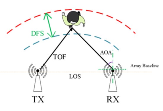
Figure 1.
CSI signal transmission scattered human (DFS—Doppler frequency shift; TOF—time of flight; AOA—angle of arrival; LOS—line of sight; Tx—transmitter; Rx—receiver).
The shortcomings of the current indoor tracking technologies are: (1) there are only three antennas at the receiving end of that ordinary equipment (e.g., Wi-Fi Link 5300 that supports 802.11 a/b/g/n), so the positioning accuracy is low; (2) there is not a strict synchronization clock for CSI signals, so the phase information received is very inaccurate; (3) performances are sensitive to multipath interferences that always exist in an indoor environment; and (4) a common MUSIC algorithm requires traversal search, which takes a lot of time.
Aiming at the problems mentioned above, we propose a new velocity and TOF estimation algorithm; Wits is simple, real-time, and accurate. It is completely different from Widar 2.0. It can effectively extract velocity information from noise/interference contaminated signals. It does not need a traversal search and has good real-time performances. It uses two sets of receiving antennas to realize trajectory tracking.
In short, the main contributions of this paper are:
- (1)
- Aiming at the problem of phase information loss caused by the phase calibration method in literature [15,19], this paper made improvements. The phase information of all antennas is retained after modification. Moreover, the algorithm reduces the random phase error;
- (2)
- According to the normal distribution of noise satisfying the mean value of 0 under normal circumstances, a velocity maximum likelihood estimation algorithm is proposed. This algorithm is completely different from Widar 2.0. No search is required. The estimation results are efficient and accurate;
- (3)
- TOF maximum likelihood estimation algorithm is proposed. Then, the TOF is used to determine the initial position;
- (4)
- Efficient and accurate position estimation and trajectory tracking are realized.
2. Materials and Methods
Wits uses 2 links in 2 groups of Rx-Tx (each receiver has 3 receiving antennas). First, the phase calibration and static path elimination are carried out at the receiving end. Then, the maximum likelihood estimation algorithm is used to estimate the radial velocity of each link. The data of the two links are finally synthesized to estimate the actual human speed. The trajectory tracking is realized using , where Δt is the time interval and is the speed. The specific process is shown in Figure 2.
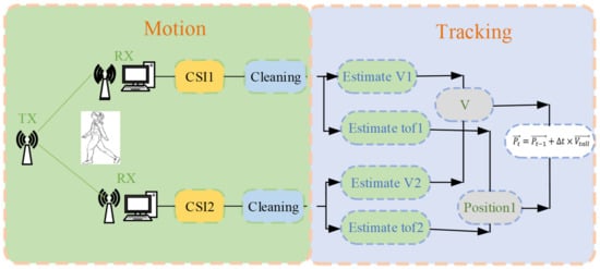
Figure 2.
Flow chart of Wits.
As shown in the previous section, Wits involves CSI modeling, phase calibration, static path elimination, and velocity estimation based on the maximum likelihood algorithm. The section describes the mathematical principle of each part of the operations.
2.1. CSI Modeling
As described before, the Wi-Fi signals propagate in space and are scattered by any object they encounter in an indoor environment. Therefore, the Wi-Fi signals’ channel state information (CSI) embodies the information about static and dynamic objects (and thus paths) in the environment. It can be expressed mathematically as:
where L represents the total number of dynamic and static paths in the environment. represents the time domain signal of path l. represents noise in the path. represents the magnitude of the signal along path l. represents the signal flight time of path l. represents the carrier frequency.
Each receiver has an antenna array, as shown in Figure 3. If the phase of the 0th subcarrier signal of the 0th packet received by the 0th antenna is taken as the reference phase (K0 in Figure 3), the phase difference of the jth subcarrier of the ith packet received by the kth antenna with respect to can be expressed as:
where refers to the frequency difference between the subcarrier j and the reference carrier; refers to the distance between the kth antenna and the reference antenna; refers to the arrival angle of the path l; c refers to the speed of light; refers to the Doppler speed of the path l; refers to the central frequency of the signal; and refers to the time interval between the ith packet and the reference data packet.
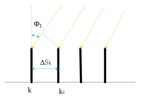
Figure 3.
Array signal diagram.
The phase difference between the jth subcarrier of the (i − 1)th packet of the kth antenna and can be expressed as:
Subtracting (2) from (3), we can get:
Based on the above analysis, the phase difference of adjacent packets carries Doppler speed information. However, the phase information received is not accurate due to imperfect hardware clock synchronization. Therefore, the corresponding phase alignment technique must be used as described below.
2.2. Phase Calibration and Static Path Elimination
Since there is no strict clock synchronization in the receiving process of CSI signal, there will be an error between the measured CSI signal and the actual CSI signal , which can be specifically expressed as:
where is time offset, is the frequency offset, and is the initial phase offset. Since the time offset and frequency offset are the same in different sensors, they can be removed by conjugate multiplication [14,18]. However, if one of the antennas is selected as the reference antenna, the phase of the antenna after alignment will be 0 by directly multiplying all antennas by the conjugate of the reference antenna. If calibrated information is used for motion recognition, useful phase information is reduced by 1/3, wasting the hardware resources. In addition to the three kinds of linear noise , , and , random noise cannot be ignored. The phase calibration method in literature [14,18] causes a waste of hardware resources and cannot remove random noise. Therefore, this paper improves the algorithm in literature [14,18]. The specific process is as follows:
Here, k stands for the kth antenna. K is the total number of antennas. Because common random noise can be approximated as Gaussian white noise with a mean of 0, the method of finding the mean can remove part of random noise by Equation (6).
where stands for all antennas. and are expressed as follows:
where represents the static path and represents the dynamic path.
Substitution of (8) and (9) into (7) reads:
The is caused by the static path and is of low frequency. is caused by the dynamic path and is of high frequency. The above two terms can be removed with a bandpass filter. The remaining two terms are expanded as follows:
By comparing (11) and (12), we can get:
Since the amplitude of the static path signal is far greater than that of the dynamic path signal , the latter can be neglected. We conducted an experiment where a person moves quickly away from an antenna and then slows down to a stop and vice versa. The results of short-time Fourier transform (STFT) before and after static elimination are shown in Figure 4a,b: in the absence of static cancellation, noise, dynamic path signal, and static path signal are mixed together and cannot be distinguished. After static elimination, there is little noise and dynamic path signal. This is very helpful for extracting accurate speed information later.
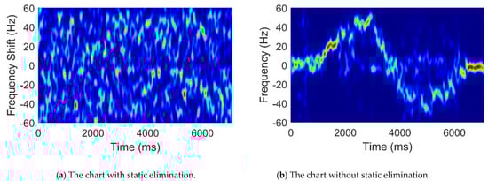
Figure 4.
The measured time–frequency chart comparison.
With the more accurate measurement of phase information and the dynamic path, the maximum likelihood estimation algorithm can be used to estimate the velocity, as described in the subsections below.
2.3. Radial Velocity Estimation Based on the Maximum Likelihood Algorithm
This algorithm is fundamentally different from Widar 2.0. Widar 2.0 mainly constructs the optimization function, traverses the amplitude, AOA, TOF, Doppler speed, and finds the minimum square error between the estimated CSI and the measured CSI. The algorithm in this paper mainly meets the requirement that the mean value is normally distributed according to the velocity estimation deviation. We divide the CSI signals collected from the network card into many segments of short window, in which the velocity is approximated considered as a constant is the number of a sliding window.
The Doppler velocity after segmentation is:
Here, is the noise and follows a Gaussian distribution with the mean of 0, and variance . A series of Doppler velocities in a short time window can be obtained by Equation (4). can be obtained by the following formula:
Here, is the frequency of jth subcarrier. The probability density function of Doppler velocity is:
The joint probability distribution function of all observed values is
represents the speed of the ith packet of the jth subcarrier of the kth antenna. V is the observed value of all velocities in segment t. I represents the total number of packets. J represents the number of total subcarriers of each antenna. K represents the total number of antennas.
The maximum likelihood estimation of velocity, namely, the logarithm, is taken to obtain the maximum probability:
The maximum likelihood estimate is obtained by taking the derivative of .
We can get rid of linear noise error caused by , , and using conjugate multiplication. is caused by random noise. Because common random noise can be approximated as Gaussian white noise with a mean of 0, the velocity obtained by formula 19 can remove the random phase noise. This is why the speed calculated by the algorithm in this paper is more accurate. We can see that the algorithm in this paper is completely different from the speed estimation algorithm in Widar 2.0. No optimal-value search is required. The algorithm proposed only needs addition and division. Therefore, the algorithm’s complexity decreases significantly, and the algorithm’s efficiency increases significantly.
Using the maximum likelihood estimation algorithm, we get the magnitude of the radial velocity of a set of antennas; however, then we are faced with the problem of how to determine its direction. We treat the sender and the receiver as the two focal points of the ellipse (Ptx and Prx), respectively, and the person (Ph) is on the ellipse. The radial velocity direction of human motion can be calculated with a set of RX-TX [15].
The specific calculation method of radial velocity is shown in Equation (20):
where represents the current position vector of the moving target. represents the vector where the transmitting antenna is located. represents the position vector of receiving antenna RX1. represents the magnitude of the radial velocity of the ellipse consisting of TX and RX1 calculated by the maximum likelihood estimation algorithm, and represents its direction.
If only one pair of transmitting and receiving antennas can measure the radial velocity of a moving object, as shown in Figure 5, how can the actual velocity be obtained? The answer is that two sets of antennas need to be used. Another set of velocities can be obtained by the same method.
where represents the so-called position vector of receiving antenna rx1. represents the magnitude of the radial velocity of the ellipse consisting of tx and rx2 calculated by the maximum likelihood estimation algorithm, and represents its direction.
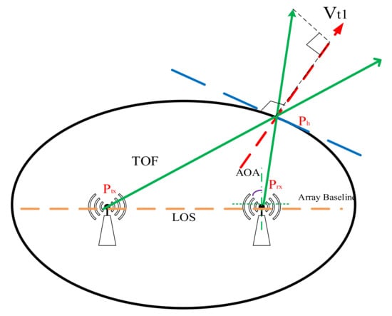
Figure 5.
Velocity direction calculation model.
The total velocities can be expressed as:
Using speed and previous time position, accurate positioning can be achieved:
represents the coordinates of the current position. represents the position of the previous time. represents the time interval between adjacent moments.
2.4. Initial Position Estimation Based on Maximum Likelihood Algorithm
With only speed information but no initial position, it is still impossible to locate and track. Therefore, this paper proposes TOF estimation based on maximum likelihood. Based on the previous information, the phase difference of the (j − 1)th subcarrier of the ith packet received by the kth antenna with respect to can be expressed as:
Subtracting (2) from (24), we can get:
It can be concluded from Equation (25) that the phase difference between adjacent subcarriers carries TOF information. We take the CSI signal collected from the network card as a piece of data at its starting time. TOF in a short time can be regarded as constant .
Here, is the noise and follows a Gaussian distribution with the mean of 0, and variance . The probability density function of TOF is:
The joint probability distribution function of all observed values is:
represents the TOF of the ith packet of the jth subcarrier of the kth antenna. is TOF. I represents the total number of packets. J represents the number of total subcarriers of each antenna. K represents the total number of antennas.
The maximum likelihood estimation of TOF, namely, the logarithm, is taken to get the maximum probability:
The maximum likelihood estimate is obtained by taking the derivative of .
The unique location cannot be determined by only one TOF of a single set of transceiver antennas. Two groups of receiving antennas are used, and their positions are as shown in Figure 6: Ptx is the transmitting antenna. Prx1 and Prx2 stand for different groups of receiving antennas. TOF1 is the time required for the signal to travel from the transmitting device Ptx to the moving target and then to Prx1. TOF2 is the time required by the signal from the transmitting device Ptx to the moving target and then to Prx2.
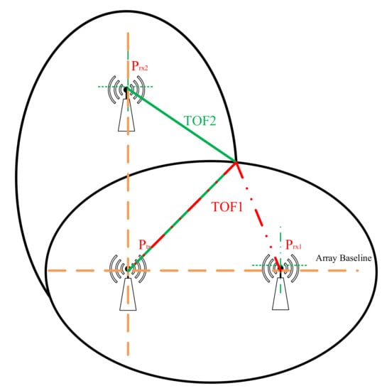
Figure 6.
Schematic diagram of starting position determination.
The intersection of the ellipses determined by the two sets of receiving antennas is unique in the detection area.
3. Results
3.1. Experiments Settings
We used two pairs of transceiver antennas, two receivers, and one transmitter. Two laptops were connected to the receivers for data processing and one desktop to the transmitter. Every receiver had three sets of antennas, forming a linear antenna array with an element spacing of 0.026 m (half wavelength). The signal was on channel 165, and the center frequency was 5.825 GHz.
In order to verify the accuracy of the algorithm, we chose two different experimental environments: a complex environment (Environment 1) with a lot of experimental equipment, tables, and chairs, and Environment 2, an empty hall. They are shown in Figure 7a,b below.
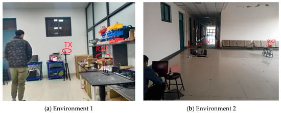
Figure 7.
The experimental environments.
3.2. Accuracy of Doppler Velocity Estimation
To verify the accuracy of the algorithm in this paper, we used the data of Classroom (environment) in Tsinghua Widar 2.0. The accuracy of Wits is compared with that of Wider 2.0 and IndoTrack, respectively, as shown in Figure 8.
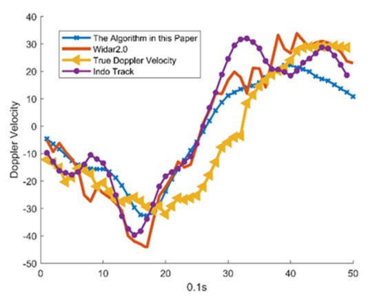
Figure 8.
Comparison of Doppler velocities of different algorithms.
Figure 9 is the error accumulation function. The maximum Doppler velocity error is 24 Hz less than the other two algorithms. It can be seen that the algorithm in this paper has good stability. The mean error of Doppler velocity is 9.34 Hz with Wits, 10.06 Hz with IndoTrack, and 10.32 Hz with Widar 2.0. The mean error of Wits in this paper is the smallest. In addition, Wits estimated a maximum Doppler velocity error of 24 Hz, Widar 2.0, and Indo track of 30 Hz and 35 Hz, respectively. Therefore, the stability and accuracy of the proposed algorithm are slightly better than existing algorithms.
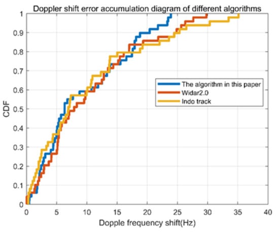
Figure 9.
Error accumulation diagram of different algorithms.
In addition, we compared the computing time of three different algorithms, as shown in Table 2. Wits is advantageous in terms of computing time and real-time performance. The reasons are as follows: IndoTrack uses the MUSIC algorithm and needs to conduct a one-dimensional search, so it takes a long time. Widar 2.0 estimates four parameters simultaneously, requiring a four-dimensional search. Although expectation-maximization is used to reduce the computation time, multiple parameters need to be estimated, so the computation time is relatively long. Especially when the number of packets is relatively large, Wits has obvious advantages. As shown in the table below, when the number of packets is 7000, Wits only needs 355 ms, while IndoTrack requires 6061 ms. IndoTrack takes 17 times more computational time than Wits. Widar 2.0 requires 7366 ms, which is 21 times as much as that by Wits.
Table 2.
The computational time of different algorithms.
3.3. Estimation of Trajectory Accuracy
- (1)
- Tracking with the known starting position.
In order to verify the positioning accuracy of this algorithm, we collected a large number of tracking data in the two environments.
The heights of the volunteers range from 158 to 178 cm. There are horizontal line track, vertical line track, U-shaped track, rectangular track, V-shaped track, and other tracks. Figure 10a,b is the trajectory prediction of a person walking along the U-shaped track and the vertical line track in Environment 1. The mean error of different trajectories in Environment 1 is 0.27 m. The maximum error of different trajectories in Environment 1 is 1 m.
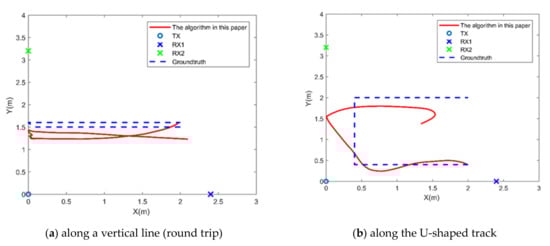
Figure 10.
The trajectory prediction of a person walking in Environment 1.
Figure 11a,b is the measured trajectories of a person walking along with the circular and the vertical line tracks in Environment 2. The mean error of different trajectories in Environment 2 is 0.20 m. The maximum error of different trajectories in Environment 2 is 0.50 m. Environment 2 does not have any furniture. Compared with Environment 1, Environment 2 has much less multipath, so the average error is smaller.
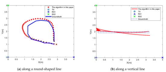
Figure 11.
The trajectory prediction of a person walking in Environment 2.
Figure 12 is the cumulative distribution function (CDF) of the tracking error in the two environments. Environment 2 is an empty and simple environment while Environment 1 is a complex environment. Experimental results show that the algorithm proposed in this paper can achieve good tracking and location results in both environments.
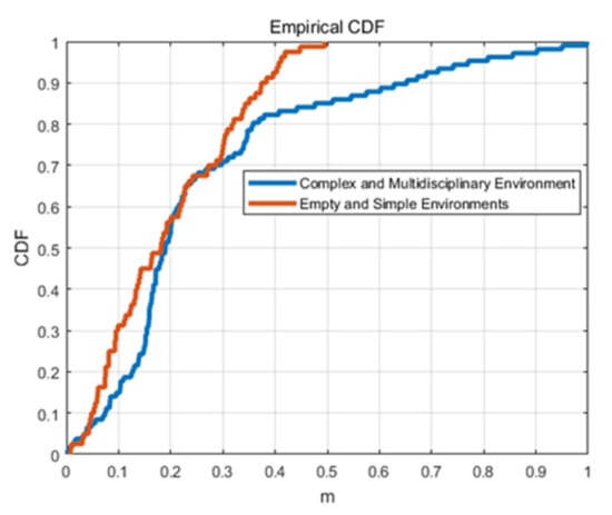
Figure 12.
Error accumulation diagram of the trajectory errors in Environment 1 and Environment 2.
- (2)
- Tracking with unknown the starting position.
The previous analysis is of the errors in two different environments with a known starting point. Then, the results were obtained with the unknown starting point. Figure 13 shows the track results in the case of Environment 1: the path is a vertical line in Figure 13a, and its average error is 0.4663 m. The path is U-shaped in Figure 13b, and its average error is 0.4652 m.
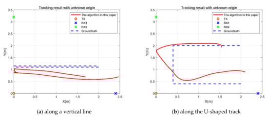
Figure 13.
The trajectory prediction of a person walking in Environment 1.
Figure 14 shows the track results in the case of Environment 2 with unknown origin: the path is a vertical line in Figure 13a, and its average error is 0.4447 m. The path is round-shaped in Figure 13b, and its average error is 0.4397 m.
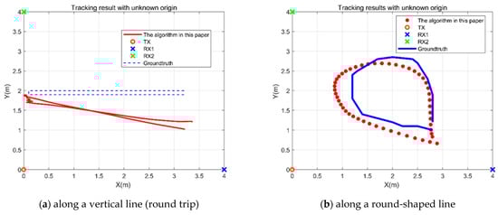
Figure 14.
The trajectory prediction of a person walking in Environment 2.
In order to verify the positioning and tracking estimation of Wits in the case of complex multi-warp and occlusion, experimental scenes are added as shown in Figure 15a. This scenario is a small laboratory. The lab was packed with lab equipment and sundries, as well as a large iron locker. In addition, a barrier of 1.3 m (high) × 0.8 m (wide) was added. The experiment shows that the error of locating and tracking increases obviously when there are obstacles in Figure 15b. On the left track in the figure below, the average error of positioning is 0.13 m, as the obstacle does not directly block the visual range of receiving and receiving signals. In the remaining part of the track with occlusion, the average positioning error is 0.59 m.
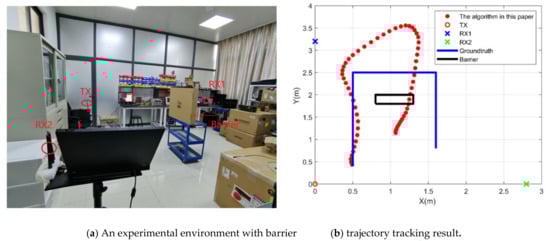
Figure 15.
The experimental environment with barrier and trajectory tracking result in this environment.
Figure 16 is the error accumulation diagram of all paths in two environments. It can be seen from the figure that the error is smaller in the environment with fewer multipath, which is consistent with the previous conclusion. The blue line is in an empty experimental environment without any furniture, so the multipath phenomenon is less, and the experimental results are more accurate. The average positioning error is 0.3452 m. The red line is the cumulative function of positioning error in a complex multipath environment. The mean positioning error in this environment is 0.4723 m. By comparison, it can be concluded that the positioning error is larger in a multipath complex environment.
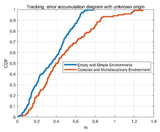
Figure 16.
Error accumulation diagram of the trajectory errors in Environment 1 and Environment 2.
Figure 17 is the CDF of the trajectory errors with different trajectory shapes. The blue line is the cumulative error of the vertical trajectory, the red line is the cumulative error of the U-shaped trajectory, and the orange line is the cumulative error of the circular trajectory. It can be seen from the figure that the trajectory error is related to the number of turns of the trajectory. When the trajectory is circular, the number of turns is largest. Therefore, the cumulative error is the largest. The errors are minimal when the trajectory is straight.
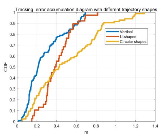
Figure 17.
Error accumulation diagram of the trajectory errors with different trajectory shapes.
Figure 18 shows the positioning error comparison between Wits and the speed-based dual-receiver antenna. The comparisons were made at an unknown starting point. The green dots and lines are the positioning error accumulation diagram of IndoTrack. The red dots and lines are the positioning error accumulation diagram of DFT-JVAE [46]. By comparison, it can be seen that the algorithm in this paper is superior to the existing system in precision.
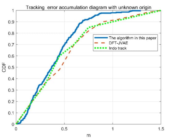
Figure 18.
Tracking error compared with different algorithm.
4. Conclusions and Discussion
In this paper, a new indoor tracking algorithm based on channel state information Wits is proposed. This algorithm mainly realizes the location by the target’s velocity. Firstly, improved algorithms were used to eliminate the interference of static paths, and to calibrate the phase information. Then, the maximum likelihood of the phase was used to estimate the velocity of the target. Experimental results show that Wits can achieve the mean error of 0.235 m in two different environments. If the starting point is unknown, the average positioning error is 0.41 m. Because the velocity is easier to obtain and more accurate than AOA and TOF detection, the tracking accuracy is higher than Widar 2.0 by Tsinghua University and IndoTrack by Peking University. In addition, Wits can remove part of the random phase noise and obtain more accurate phase information. The velocity information estimated from the phase information is also more accurate. The maximum likelihood estimation is used which can obtain accurate results in a multipath environment. The algorithm can also eliminate linear phase error and random phase error. Using a static path elimination algorithm, the interference of multipath can be reduced. If the starting point was known, the average positioning error of FDT-JVAE was 0.0.32 m, IndoTrack was 0.39 m, and Widar was 0.47 m. Compared with FDT-JVAE, the accuracy of the proposed method is improved by 26.5%. The accuracy of the proposed algorithm is 39.7% higher than that of IndoTrack. Compared with Widar, the accuracy of the proposed algorithm is improved by 50%.
It is worth mentioning that Wits essentially determines the next position based on the previous position, so there is an accumulation error. Therefore, it is necessary to continuously calibrate the system. If there are many people, and only one person moves, the others can be removed by a static elimination algorithm. If more than one person is moving, the speeds of multiple people add up, making it impossible to distinguish the movements of different people. Therefore, the situation of multi-person movement cannot be solved in this paper, temporarily. These issues are under study and the results will be reported in the future.
Author Contributions
Conceptualization, L.-P.T. and L.-Q.C.; methodology, L.-P.T.; software, L.-P.T.; validation, L.-P.T., Z.C. and Z.-M.X.; investigation, L.-P.T.; resources, Z.-M.X.; data curation, L.-Q.C.; writing—original draft preparation, Z.-M.X.; writing—review and editing, L.-P.T.; visualization, L.-P.T.; supervision, L.-Q.C.; project administration, Z.C.; funding acquisition, Z.C. All authors have read and agreed to the published version of the manuscript.
Funding
This work was supported in part by the National Natural Science Foundation of China (NSFC) No. 61401100 and 62071125, This work was supported in part the National Natural Science Foundation of China under Grant 62071125, the Industry-University-Research Collaboration Project of Fujian Province under Grant 2019H6007,the Natural Science Foundation of Fujian Province under Grant 2021J01581and 2018J01805, and the Scientific Research Foundation of Fuzhou University under Grant GXRC-18083.
Institutional Review Board Statement
Not applicable for studies not involving humans or animals.
Informed Consent Statement
Informed consent was obtained from all subjects involved in the study.
Data Availability Statement
Not applicable.
Conflicts of Interest
The authors declare no conflict of interest.
References
- Kim, J.; Jun, H. Vision-based location positioning using augmented reality for indoor navigation. IEEE Trans. Consum. Electron. 2008, 54, 954–962. [Google Scholar] [CrossRef]
- Sadeghi, H.; Valaee, S.; Shirani, S. A Weighted KNN Epipolar Geometry-Based Approach for Vision-Based Indoor Localization Using Smartphone Cameras. In Proceedings of the 2014 IEEE 8th Sensor Array and Multichannel Signal Processing Workshop (SAM), A Coruna, Spain, 22–25 June 2014; pp. 37–40. [Google Scholar] [CrossRef]
- Kazemipur, B.; Syed, Z.; Georgy, J.; El-Sheimy, N. Vision-Based Context and Height Estimation for 3D Indoor Location. In Proceedings of the 2014 IEEE/ION Position, Location and Navigation Symposium—PLANS 2014, Monterey, CA, USA, 5–8 May 2014; pp. 1336–1342. [Google Scholar] [CrossRef]
- Wang, G.; Gu, C.; Inoue, T.; Li, C. A Hybrid FMCW-interferometry radar for indoor precise positioning and versatile life activity monitoring. IEEE Trans. Microw. Theory Tech. 2014, 62, 2812–2822. [Google Scholar] [CrossRef]
- Gierlich, R.; Huettner, J.; Ziroff, A.; Weigel, R.; Huemer, M. A ReconFigureurable MIMO system for high-precision FMCW local positioning. IEEE Trans. Microw. Theory Tech. 2011, 59, 3228–3238. [Google Scholar] [CrossRef]
- Shen, X.; Zheng, H.; Feng, X. A Novel FMCW Radar-Based Scheme for Indoor Localization and Trajectory Tracking. In Proceedings of the 2020 IEEE 6th International Conference on Computer and Communications (ICCC), Chengdu, China, 11–14 December 2020; pp. 298–303. [Google Scholar] [CrossRef]
- Ahmed, S.; Jardak, S.; Alouini, M. Low Complexity Algorithms to Independently and Jointly Estimate the Location and Range of Targets Using FMCW. In Proceedings of the 2016 IEEE Global Conference on Signal and Information Processing (GlobalSIP), Washington, DC, USA, 7–9 December 2016; pp. 1072–1076. [Google Scholar] [CrossRef]
- Duan, S.; Yu, T.; He, J. WiDriver: Driver activity recognition system based on Wi-Fi CSI. Int. J. Wirel. Inf. Netw. 2018, 25, 146–156. [Google Scholar] [CrossRef]
- Feng, C.; Arshad, S.; Liu, Y. MAIS: Multiple Activity Identification System Using Channel State Information of Wi-Fi Signals. In International Conference on Wireless Algorithms, Systems, and Applications (WASA), Wireless Algorithms, Systems, and Applications; Springer: Berlin, Germany, 2017; pp. 419–432. [Google Scholar]
- Guo, L.; Wang, L.; Liu, J.; Zhou, W.; Lu, B. HuAc: Human Activity Recognition Using Crowd Sourced Wi-Fi Signals and Skeleton Data. Wirel. Commun. Mob. Comput. 2018, 2018, 6163475. [Google Scholar] [CrossRef]
- Jiang, W.; Miao, C.; Ma, F.; Yao, S.; Wang, Y.; Yuan, Y.; Xue, H.; Song, C.; Ma, X.; Koutsonikolas, D. Towards Environment Independent Device Free Human Activity Recognition. In Proceedings of the 24th Annual International Conference on Mobile Computing and Networking (MobiCom’18), New Delhi, India, 29 October–2 November 2018; pp. 289–304. [Google Scholar]
- Zhang, J.; Wei, B.; Hu, W.; Kanhere, S.S. WiFi-ID: Human Identification Using Wi-Fi signal. In Proceedings of the 2016 International Conference on Distributed Computing in Sensor Systems (DCOSS), Washington, DC, USA, 26–28 May 2016; pp. 75–82. [Google Scholar]
- Zeng, Y.; Pathak, P.H.; Mohapatra, P. WiWho: WiFi-Based Person Identification in Smart Spaces. In Proceedings of the 2016 15th ACM/IEEE International Conference on Information Processing in Sensor Networks (IPSN), Vienna, Austria, 11–14 April 2016; pp. 1–12. [Google Scholar]
- Ali, K.; Liu, A.X.; Wang, W.; Shahzad, M. Keystroke Recognition Using Wi-Fi Signals. In Proceedings of the 21st Annual International Conference on Mobile Computing and Networking (MobiCom’15), Paris, France, 7–11 September 2015; pp. 90–102. [Google Scholar]
- Xu, C.; Firner, B.; Moore, R.S.; Zhang, Y.; Trappe, W.; Howard, R.; Zhang, F.; An, N. Scpl: Indoor Device-Free Multi-Subject Counting and Localization Using Radio Signal Strength. In Proceedings of the ACM/IEEE International Conference on Information Processing in Sensor Networks (IPSN), Philadelphia, PA, USA, 8–11 April 2013; pp. 79–90. [Google Scholar]
- Seifeldin, M.; Saeed, A.; Kosba, A.E.; El-Keyi, A.; Youssef, M. Nuzzer: A large-scale device-free passive localization system for wireless environments. IEEE Trans. Mob. Comput. 2013, 12, 1321–1334. [Google Scholar] [CrossRef] [Green Version]
- Xi, W.; Zhao, J.; Li, X.Y.; Zhao, K.; Tang, S.; Liu, X.; Jiang, Z. Electronic Frog Eye: Counting Crowd Using Wi-Fi. In Proceedings of the IEEE INFOCOM 2014—IEEE Conference on Computer Communications, Toronto, ON, Canada, 27 April–2 May 2014; pp. 361–369. [Google Scholar]
- Wang, X.Y.; Yan, C.; Mao, S.W. PhaseBeat: Exploiting CSI Phase Data for Vital Sign Monitoring with Commodity Wi-Fi Devices. In Proceedings of the 2017 IEEE 37th International Conference on Distributed Computing Systems, Atlanta, GA, USA, 5–8 June 2017; pp. 1230–1239. [Google Scholar]
- Liu, J.; Chen, Y.; Wang, Y.; Chen, X.; Cheng, J.; Yang, J. Monitoring vital signs and postures during sleep using Wi-Fi signals. IEEE Internet Things J. 2018, 5, 2071–2083. [Google Scholar] [CrossRef]
- Wang, H.; Zhang, D.; Ma, J.; Wang, Y.; Wang, Y.; Wu, D.; Gu, T.; Xie, B. Human Respiration Detection with Commodity Wi-Fi Devices: Do User Location and Body Orientation Matter? In Proceedings of the 2016 ACM International Joint Conference on Pervasive and Ubiquitous Computing (UbiComp 2016), Heidelberg, Germany, 12–16 September 2016; pp. 25–36. [Google Scholar]
- Zhang, D.; Hu, Y.; Chen, Y.; Zeng, B. Breath track: Tracking indoor human breath status via commodity Wi-Fi. IEEE Internet Things J. 2019, 2, 3899–3911. [Google Scholar] [CrossRef]
- Lee, S.; Park, Y.D.; Suh, Y.J.; Jeon, S. Design and Implementation of Monitoring System for Breathing and Heart Rate Pattern Using Wi-Fi Signals. In Proceedings of the 15th IEEE Annual Consumer Communications & Networking Conference (CCNC), Las Vegas, NV, USA, 12–15 January 2018; pp. 2331–9860. [Google Scholar]
- Kotaru, M.; Joshi, K.; Bharadia, D.; Katti, S. SpotFi: Decimeter Level Localization Using Wi-Fi. In Proceedings of the SIGCOMM ‘15: Proceedings of the 2015 ACM Conference on Special Interest Group on Data Communication, London, UK, 17–21 August 2015. [Google Scholar]
- Kotaru, M.; Katti, S. Position Tracking for Virtual Reality Using Commodity Wi-Fi. In Proceedings of the 2017 IEEE Conference on Computer Vision and Pattern Recognition (CVPR), Honolulu, HI, USA, 21–26 July 2017; pp. 2671–2681. [Google Scholar] [CrossRef] [Green Version]
- Xiao, N.; Yang, P.; Li, X.; Zhang, Y.; Yan, Y.; Zhou, H. MilliBack: Real-Time Plug-n-Play Millimeter Level Tracking Using Wireless Backscattering. In ACM on Interactive, Mobile, Wearable and Ubiquitous Technologies; Association for Computing Machinery: New York, NY, USA, 2019. [Google Scholar]
- Shu, Y.; Huang, Y.; Zhang, J.; Coué, P.; Cheng, P.; Chen, J.; Shin, K.G. Gradient-based fingerprinting for indoor localization and tracking. IEEE Trans. Ind. Electron. 2016, 63, 2424–2433. [Google Scholar] [CrossRef]
- Wang, X.; Gao, L.; Mao, S.; Pandey, S. CSI-based fingerprinting for indoor localization: A deep learning approach. IEEE Trans. Veh. Technol. 2017, 66, 763–776. [Google Scholar] [CrossRef] [Green Version]
- Sun, W.; Xue, M.; Yu, H.; Tang, H.; Lin, A. Augmentation of fingerprints for indoor wi-fi localization based on gaussian process regression. IEEE Trans. Veh. Technol. 2018, 67, 10896–10905. [Google Scholar] [CrossRef]
- Shi, S.; Sigg, S.; Chen, L.; Ji, Y. Accurate location tracking from CSI-based passive device-free probabilistic fingerprinting. IEEE Trans. Veh. Technol. 2018, 67, 5217–5230. [Google Scholar] [CrossRef] [Green Version]
- Sánchez-Rodríguez, D.; Quintana-Suárez, M.A.; Alonso-González, I.; Ley-Bosch, C.; Sánchez-Medina, J.J. Fusion of channel state information and received signal strength for indoor localization using a single access point. Remote Sens. 2020, 12, 1995. [Google Scholar] [CrossRef]
- Haider, A.; Wei, Y.; Liu, S.; Hwang, S.H. Pre- and post-processing algorithms with deep learning classifier for Wi-Fi fingerprint-based indoor positioning. Electronics 2019, 8, 195. [Google Scholar] [CrossRef] [Green Version]
- Wang, X.; Wang, X.; Mao, S. Deep convolutional neural networks for indoor localization with CSI images. IEEE Trans. Netw. Sci. Eng. 2020, 7, 316–327. [Google Scholar] [CrossRef]
- Jing, Y.; Hao, J.; Li, P. Learning spatiotemporal features of CSI for indoor localization with dual-stream 3D convolutional neural networks. IEEE Access 2019, 7, 147571–147585. [Google Scholar] [CrossRef]
- Li, P.; Li, P.; Cui, H.; Khan, A.; Raza, U.; Piechocki, R.; Doufexi, A.; Farnham, T. Deep Transfer Learning for WiFi Localization. In IEEE Radar Conference (RadarConf21); IEEE: Piscataway, NJ, USA, 2021. [Google Scholar]
- Wang, X.; Gao, L.; Mao, S. PhaseFI: Phase Fingerprinting for Indoor Localization with a Deep Learning Approach. In Proceedings of the IEEE Global Commun. Conf. (GLOBECOM), San Diego, CA, USA, 6–10 December 2015; pp. 1–6. [Google Scholar]
- Zhou, M.; Long, Y.; Zhang, W.; Pu, Q.; Wang, Y.; Nie, W.; He, W. Adaptive Genetic Algorithm-aided Neural Network with Channel State Information Tensor Decomposition for Indoor Localization. IEEE Trans. Evol. Comput. 2021, 99. [Google Scholar] [CrossRef]
- Zhu, X.; Qiu, T.; Qu, W.; Zhou, X.; Atiquzzaman, M.; Wu, D. BLS-location: A wireless fingerprint localization algorithm based on broad learning. IEEE Trans. Mob. Comput. 2021, 99. [Google Scholar] [CrossRef]
- Zhang, Y.; Wang, W.; Xu, C.; Qin, J.; Yu, S.; Zhang, Y. SICD: Novel single-access-point indoor localization based on CSI-MIMO with dimensionality reduction. Sensors 2021, 21, 1325. [Google Scholar] [CrossRef] [PubMed]
- He, Y.; Chen, Y.; Hu, Y.; Zeng, B. WiFi vision: Sensing, recognition, and detection with commodity MIMO-OFDM WiFi. IEEE Internet Things J. 2020, 7, 8296–8317. [Google Scholar] [CrossRef]
- Li, X.; Zhang, D.; Lv, Q.; Xiong, J.; Li, S.; Zhang, Y.; Mei, H. IndoTrack: Device-Free Indoor Human Tracking with Commodity Wi-Fi. In Proceedings of the ACM on Interactive, Mobile, Wearable and Ubiquitous Technologies; Association for Computing Machinery: New York, NY, USA, 2017. [Google Scholar]
- Li, X.; Li, S.; Zhang, D.; Xiong, J.; Wang, Y.; Mei, H. Dynamic-Music: Accurate Device-Free Indoor Localization. In Proceedings of the 2016 ACM International Joint Conference on Pervasive and Ubiquitous Computing, Heidelberg, Germany, 12–16 September 2016; Association for Computing Machinery: New York, NY, USA, 2016. [Google Scholar]
- Joshi, K.; Bharadia, D.; Kotaru, M.; Katti, S. Wideo: Fine-Grained Device-Free Motion Tracing Using RF Backscatter. In Proceedings of the 12th {USENIX} Symposium on Networked Systems Design and Implementation ({NSDI} 15), Oakland, CA, USA, 4–6 May 2015. [Google Scholar]
- Qian, K.; Wu, C.; Yang, Z.; Liu, Y.; Jamieson, K. Widar: Decimeter-Level Passive Tracking via Velocity Monitoring with Commodity Wi-Fi. In Proceedings of the 18th ACM International Symposium on Mobile Ad Hoc Networking and Computing, Chennai, India, 10–14 July 2017; Association for Computing Machinery: New York, NY, USA, 2017. [Google Scholar]
- Qian, K.; Wu, C.; Zhang, Y.; Zhang, G.; Yang, Z.; Liu, Y. Widar2.0: Passive Human Tracking with a Single Wi-Fi Link. In Proceedings of the 16th Annual International Conference on Mobile Systems, Applications, and Services, Munich, Germany, 10–15 June 2018; Association for Computing Machinery: New York, NY, USA, 2018. [Google Scholar]
- Wang, J.; Jiang, H.; Xiong, J.; Jamieson, K.; Chen, X.; Fang, D.; Xie, B. LiFS: Low Human-effort, Device-free Localization with Fine-grained Subcarrier Information. In Proceedings of the 22nd Annual International Conference on Mobile Computing and Networking, New York, NY, USA, 3–7 October 2016; Association for Computing Machinery: New York, NY, USA. [Google Scholar]
- Zhang, L.; Wang, H. Device-free tracking via joint velocity and AOA estimation with commodity WiFi. IEEE Sens. J. 2019, 19, 10662–10673. [Google Scholar] [CrossRef]
Publisher’s Note: MDPI stays neutral with regard to jurisdictional claims in published maps and institutional affiliations. |
© 2021 by the authors. Licensee MDPI, Basel, Switzerland. This article is an open access article distributed under the terms and conditions of the Creative Commons Attribution (CC BY) license (https://creativecommons.org/licenses/by/4.0/).