
A Deep Multitask Semisupervised Learning Approach for Chlorophyll-a Retrieval from Remote Sensing Images


Abstract
:
1. Introduction
1.1. Related Work
1.2. Aim and Contribution
2. Materials and Methods
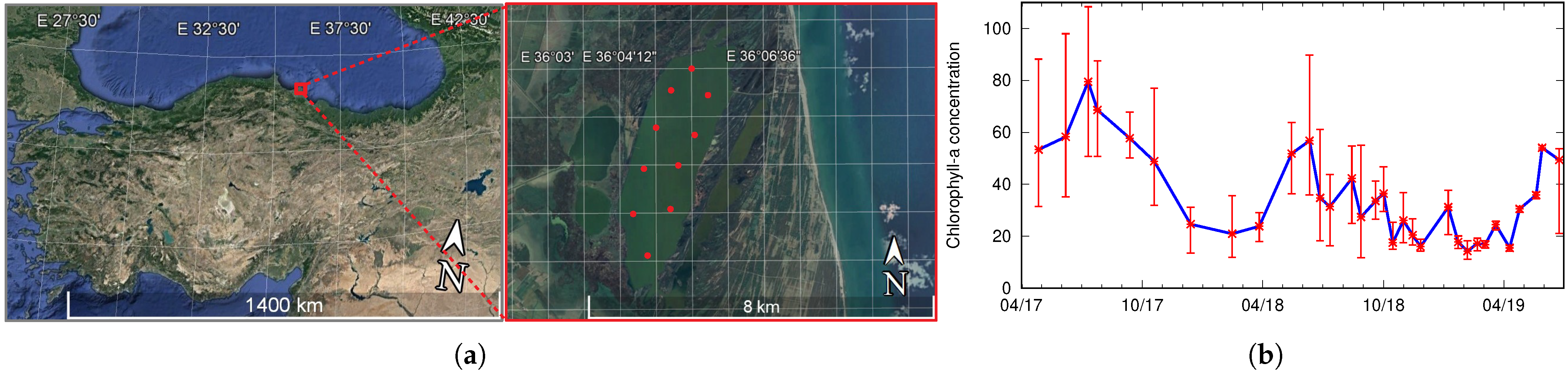
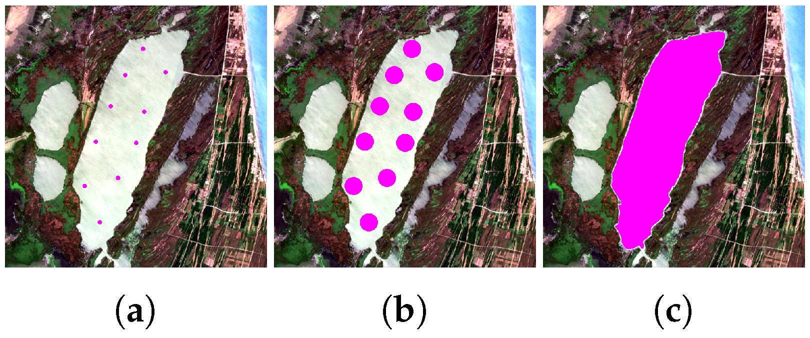
2.1. Study Area and Data
2.2. Proposed Method
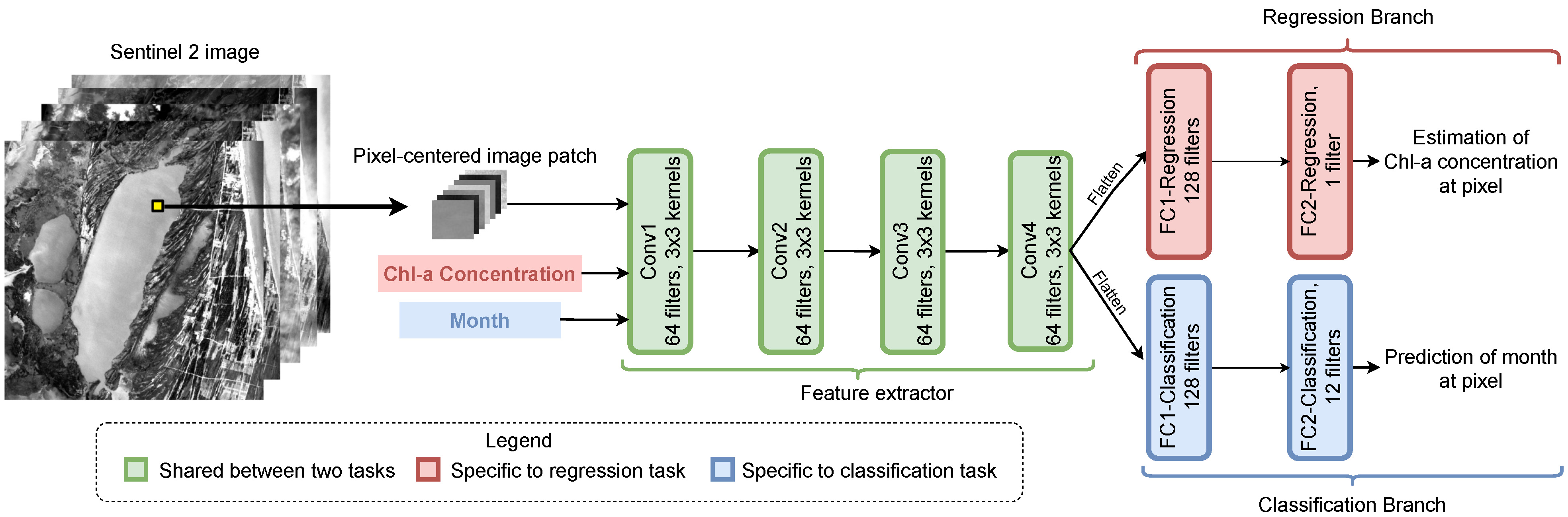
2.2.1. Input Shape
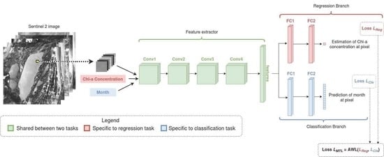
2.2.2. Network Architecture
2.2.3. Loss Functions
2.2.4. Multitask Loss
3. Results and Discussion
3.1. Data Split
3.2. Setup
3.3. Training
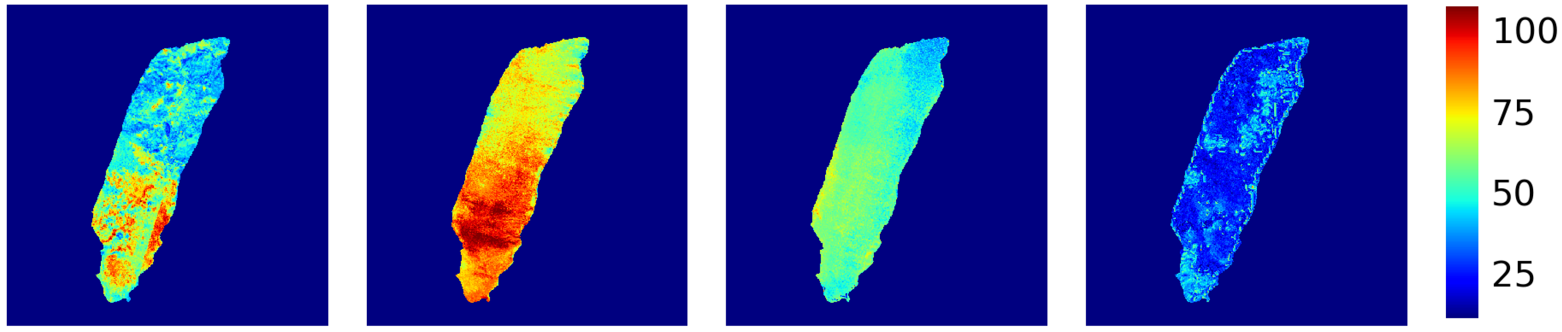
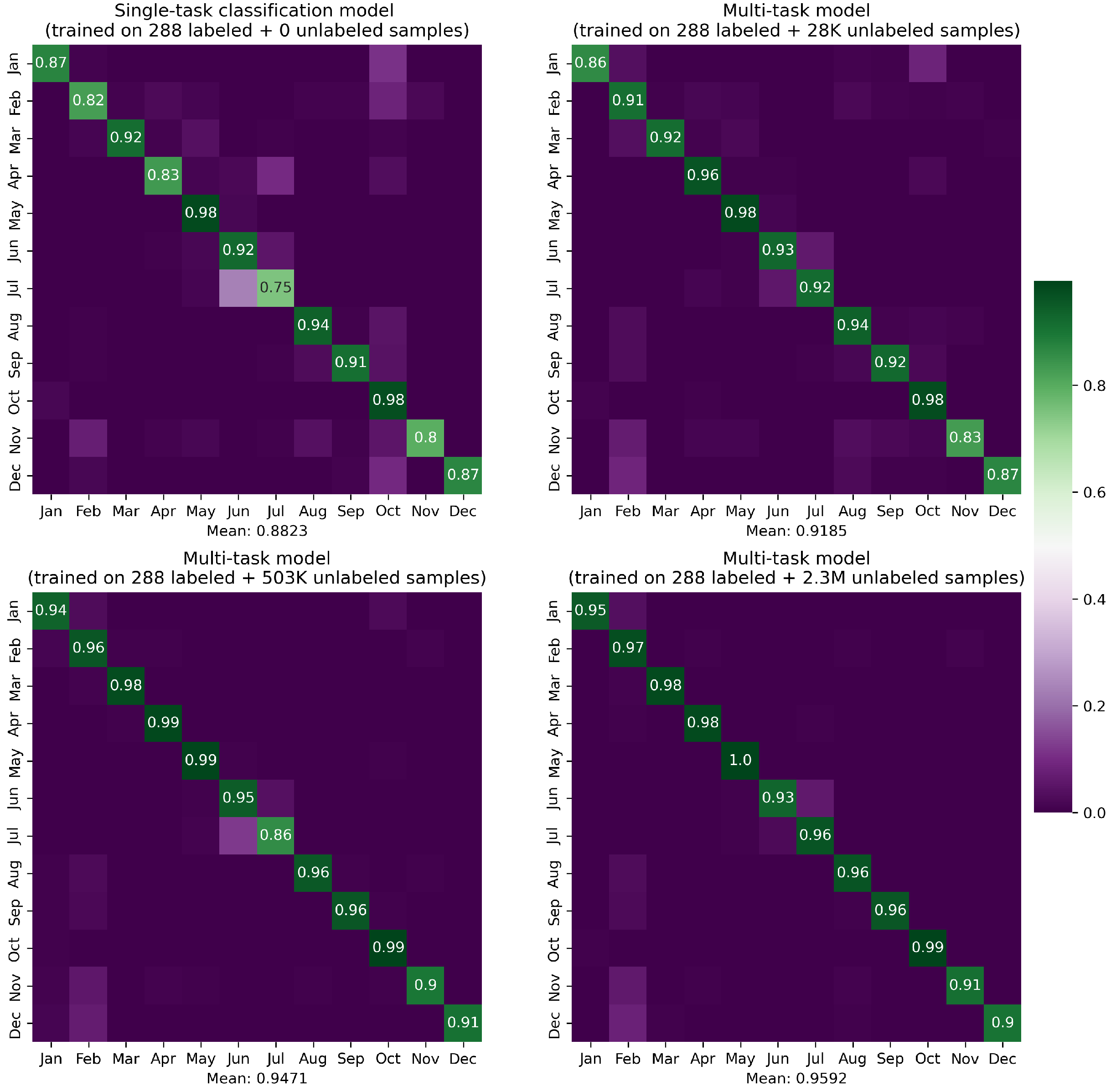
3.4. Results
3.5. Ablation Study
3.6. Discussion and Limitations
4. Conclusions
Author Contributions
Funding
Institutional Review Board Statement
Informed Consent Statement
Data Availability Statement
Conflicts of Interest
References
- Caballero, I.; Steinmetz, F.; Navarro, G. Evaluation of the first year of operational sentinel-2A data for retrieval of suspended solids in medium- to high-turbidity waters. Remote Sens. 2018, 10, 982. [Google Scholar] [CrossRef] [Green Version]
- Kane, D.D.; Conroy, J.D.; Richards, R.P.; Baker, D.B.; Culver, D.A. Re-eutrophication of Lake Erie: Correlations between tributary nutrient loads and phytoplankton biomass. J. Great Lakes Res. 2014, 40, 496–501. [Google Scholar] [CrossRef]
- Brooks, B.W.; Lazorchak, J.M.; Howard, M.D.; Johnson, M.V.V.; Morton, S.L.; Perkins, D.A.; Reavie, E.D.; Scott, G.I.; Smith, S.A.; Stevens, J.A. Are harmful algal blooms becoming the greatest inland water quality threat to public health and aquatic ecosystems? Environ. Toxicol. Chem. 2016, 35, 6–13. [Google Scholar] [CrossRef] [PubMed]
- Ritchie, J.C.; Zimba, P.V.; Everitt, J.H. Remote sensing techniques to assess water quality. Photogramm. Eng. Remote Sens. 2003, 69, 695–704. [Google Scholar] [CrossRef] [Green Version]
- Laliberté, J.; Larouche, P.; Devred, E.; Craig, S. Chlorophyll-a Concentration Retrieval in the Optically Complex Waters of the St. Lawrence Estuary and Gulf Using Principal Component Analysis. Remote Sens. 2018, 10, 265. [Google Scholar] [CrossRef] [Green Version]
- Cui, T.W.; Zhang, J.; Wang, K.; Wei, J.W.; Mu, B.; Ma, Y.; Zhu, J.H.; Liu, R.J.; Chen, X.Y. Remote sensing of chlorophyll a concentration in turbid coastal waters based on a global optical water classification system. ISPRS J. Photogramm. Remote Sens. 2020, 163, 187–201. [Google Scholar] [CrossRef]
- Johansen, R.; Beck, R.; Nowosad, J.; Nietch, C.; Xu, M.; Shu, S.; Yang, B.; Liu, H.; Emery, E.; Reif, M.; et al. Evaluating the portability of satellite derived chlorophyll-a algorithms for temperate inland lakes using airborne hyperspectral imagery and dense surface observations. Harmful Algae 2018, 76, 35–46. [Google Scholar] [CrossRef]
- Pahlevan, N.; Smith, B.; Schalles, J.; Binding, C.; Cao, Z.; Ma, R.; Alikas, K.; Kangro, K.; Gurlin, D.; Hà, N.; et al. Seamless retrievals of chlorophyll-a from Sentinel-2 (MSI) and Sentinel-3 (OLCI) in inland and coastal waters: A machine-learning approach. Remote Sens. Environ. 2020, 240, 111604. [Google Scholar] [CrossRef]
- Dörnhöfer, K.; Oppelt, N. Remote sensing for lake research and monitoring—Recent advances. Ecol. Indic. 2016, 64, 105–122. [Google Scholar] [CrossRef]
- Huang, C.; Chen, X.; Li, Y.; Yang, H.; Sun, D.; Li, J.; Le, C.; Zhou, L.; Zhang, M.; Xu, L. Specific inherent optical properties of highly turbid productive water for retrieval of water-quality after optical classification. Environ. Earth Sci. 2015, 73, 1961–1973. [Google Scholar] [CrossRef]
- Giardino, C.; Oggioni, A.; Bresciani, M.; Yan, H. Remote sensing of suspended particulate matter in Himalayan lakes. Mt. Res. Dev. 2010, 30, 157–168. [Google Scholar] [CrossRef]
- Lan, X.; Guo, Z.; Tian, Y.; Lei, X.; Wang, J. Retrieval of water quality parameters by neural network and analytical algorithm in Guanting Reservoir in Hebei Province in China. In Proceedings of the IEEE International Geoscience and Remote Sensing Symposium, Milan, Italy, 26–31 July 2015; pp. 723–726. [Google Scholar]
- Verrelst, J.; Rivera, J.P.; Gitelson, A.; Delegido, J.; Moreno, J.; Camps-Valls, G. Spectral band selection for vegetation properties retrieval using Gaussian processes regression. Int. J. Appl. Earth Obs. Geoinf. 2016, 52, 554–567. [Google Scholar] [CrossRef]
- Vilas, L.G.; Spyrakos, E.; Palenzuela, J.M.T. Neural network estimation of chlorophyll a from MERIS full resolution data for the coastal waters of Galician rias (NW Spain). Remote Sens. Environ. 2011, 115, 524–535. [Google Scholar] [CrossRef]
- Wang, X.; Ma, L.; Wang, X. Apply semi-supervised support vector regression for remote sensing water quality retrieving. In Proceedings of the IEEE International Geoscience and Remote Sensing Symposium, Honolulu, HI, USA, 25–30 July 2010; pp. 2757–2760. [Google Scholar]
- Ansper, A.; Alikas, K. Retrieval of Chlorophyll a from Sentinel-2 MSI Data for the European Union Water Framework Directive Reporting Purposes. Remote Sens. 2019, 11, 64. [Google Scholar] [CrossRef] [Green Version]
- O’Reilly, J.E.; Maritorena, S.; Mitchell, B.G.; Siegel, D.A.; Carder, K.L.; Garver, S.A.; Kahruand, M.; McClain, C. Ocean color chlorophyll algorithms for SeaWiFS. J. Geophys. Res. 1998, 103, 24937–24953. [Google Scholar] [CrossRef] [Green Version]
- Freitas, F.H.; Dierssen, H.M. Evaluating the seasonal and decadal performance of red band difference algorithms for chlorophyll in an optically complex estuary with winter and summer blooms. Remote Sens. Environ. 2019, 231, 111228. [Google Scholar] [CrossRef]
- Matthews, M.W.; Bernard, S.; Robertson, L. An algorithm for detecting trophic status (chlorophyll-a), cyanobacterial-dominance, surface scums and floating vegetation in inland and coastal waters. Remote Sens. Environ. 2012, 124, 637–652. [Google Scholar] [CrossRef]
- Pahlevan, N.; Sarkara, S.; Franza, B.A.; Balasubramanian, S.V.; Hec, J. Sentinel-2 multispectral instrument (MSI) data processing for aquatic science applications: Demonstrations and validations. Remote Sens. Environ. 2017, 201, 47–56. [Google Scholar] [CrossRef]
- Niroumand-Jadidi, M.; Bovolo, F.; Bruzzone, L. Novel Spectra-Derived Features for Empirical Retrieval of Water Quality Parameters: Demonstrations for OLI, MSI, and OLCI Sensors. IEEE Trans. Geosci. Remote Sens. 2019, 57, 10285–10300. [Google Scholar] [CrossRef]
- Aptoula, E.; Ariman, S. Hierarchical Spatial-Spectral Features for the Chlorophyll-a Estimation of Lake Balik, Turkey. IEEE Geosci. Remote. Sens. Lett. 2020, 19, 1500405. [Google Scholar] [CrossRef]
- Neil, C.; Spyrakos, E.; Hunter, P.D.; Tyler, A.N. A global approach for chlorophyll-a retrieval across optically complex inland waters based on optical water types. Remote Sens. Environ. 2019, 229, 159–178. [Google Scholar] [CrossRef]
- Hinton, G.E.; Salakhutdinov, R.R. Reducing the dimensionality of data with neural networks. Science 2006, 313, 504–507. [Google Scholar] [CrossRef] [Green Version]
- Krizhevsky, A.; Sutskever, I.; Hinton, G.E. ImageNet classification with deep convolutional neural networks. In Proceedings of the International Conference on Neural Information Processing Systems, Lake Tahoe, NV, USA, 3–6 December 2012; Volume 1, pp. 1097–1105. [Google Scholar]
- Ma, L.; Liu, Y.; Zhang, X.; Ye, Y.; Yin, G.; Johnson, B.A. Deep learning in remote sensing applications: A meta-analysis and review. ISPRS J. Photogramm. Remote Sens. 2019, 152, 166–177. [Google Scholar] [CrossRef]
- Peterson, K.T.; Sagan, V.; Sloan, J.J. Deep learning-based water quality estimation and anomaly detection using Landsat-8/Sentinel-2 virtual constellation and cloud computing. GIScience Remote Sens. 2020, 57, 510–525. [Google Scholar] [CrossRef]
- Pu, F.; Ding, C.; Chao, Z.; Yu, Y.; Xu, X. Water-Quality Classification of Inland Lakes Using Landsat-8 Images by Convolutional Neural Networks. Remote Sens. 2019, 11, 1674. [Google Scholar] [CrossRef] [Green Version]
- Aptoula, E.; Ariman, S. Chlorophyll-a Retrieval From Sentinel-2 Images Using Convolutional Neural Network Regression. IEEE Geosci. Remote Sens. Lett. 2021, 1–5. [Google Scholar] [CrossRef]
- Syariz, M.; Lin, C.; Nguyen, M.; Jaelani, L.; Blanco, A. WaterNet: A Convolutional Neural Network for Chlorophyll-a Concentration Retrieval. Remote Sens. 2020, 12, 1966. [Google Scholar] [CrossRef]
- Cho, H.; Choi, U.; Park, H. Deep Learning Application to Time Series Prediction of Daily Chlorophyll-a Concentration. WIT Trans. Ecol. Environ. 2018, 215, 157–163. [Google Scholar]
- Barzegar, R.; Aalami, M.; Adamowski, J. Short-term water quality variable prediction using a hybrid CNN–LSTM deep learning model. Stoch. Environ. Res. Risk Assess. 2020, 34, 415–433. [Google Scholar] [CrossRef]
- General Directorate for the Protection of Natural Assets. Samsun Kizilirmak Deltasi Sulak Alan Ve Kus Cenneti Dogal Sit Alanlari Yonetim Plani; Technical Report; Ministry of Environment and Urban Planning: Ankara, Turkey, 2017.
- Arar, E.J.; Collins, G.B. Method 445.0 In Vitro Determination of Chlorophyll-a and Pheophytin-a in Marine and Freshwater Algae by Fluorescence; Technical Report; U.S. Environmental Protection Agency: Washington, DC, USA, 1997.
- Organization for Economic Co-operation and Development. Eutrophication of Waters: Monitoring, Assessment and Control; Organization for Economic Co-Operation and Development: Washington, DC, USA, 1982. [Google Scholar]
- Steinmetz, F.; Deschamps, P.Y.; Ramon, D. Atmospheric correction in presence of sun glint: Application to MERIS. Opt. Express 2011, 19, 9783–9800. [Google Scholar] [CrossRef] [Green Version]
- Pereira-Sandoval, M.; Ruescas, A.; Urrego, P.; Ruiz-Verdu, A.; Delegido, J.; Tenjo, C.; Soria-Perpinya, X.; Vicente, E.; Soria, J.; Moreno, J. Evaluation of Atmospheric Correction Algorithms over Spanish Inland Waters for Sentinel-2 Multi Spectral Imagery Data. Remote Sens. 2019, 11, 1469. [Google Scholar] [CrossRef] [Green Version]
- Son, S.; Wang, M. Water properties in Chesapeake Bay from MODIS-Aqua measurements. Remote Sens. Environ. 2012, 123, 163–174. [Google Scholar] [CrossRef] [Green Version]
- Choi, J.; Kim, J.; Won, J.; Min, O. Modelling Chlorophyll-a Concentration using Deep Neural Networks considering Extreme Data Imbalance and Skewness. In Proceedings of the IEEE International Conference on Advanced Communication Technology (ICACT), PyeongChang, Korea, 17–20 February 2019; pp. 631–634. [Google Scholar]
- Kendall, A.; Gal, Y.; Cipolla, R. Multi-task Learning Using Uncertainty to Weigh Losses for Scene Geometry and Semantics. In Proceedings of the IEEE/CVF Conference on Computer Vision and Pattern Recognition (CVPR), Salt Lake City, UT, USA, 18–23 June 2018; pp. 7482–7491. [Google Scholar]
- Liebel, L.; Körner, M. Auxiliary Tasks in Multi-task Learning. arXiv 2018, arXiv:1805.06334. [Google Scholar]
- Batur, E.; Maktav, D. Assessment of Surface Water Quality by Using Satellite Images Fusion Based on PCA Method in the Lake Gala, Turkey. IEEE Trans. Geosci. Remote Sens. 2019, 57, 2983–2989. [Google Scholar] [CrossRef]


| Month | |||||||||||||
|---|---|---|---|---|---|---|---|---|---|---|---|---|---|
| 1 | 2 | 3 | 4 | 5 | 6 | 7 | 8 | 9 | 10 | 11 | 12 | Total | |
| Unlabeled | 148 K | 222 K | 222 K | 222 K | 222 K | 296 K | 222 K | 148 K | 148 K | 296 K | 148 K | 74 K | 2365 K |
| Labeled | 20 | 30 | 30 | 30 | 30 | 40 | 30 | 20 | 20 | 40 | 20 | 10 | 320 |
| Method | Dataset | MAE | RMSE | Model Parameters | |
|---|---|---|---|---|---|
| Band ratio [16] | Labeled | 71.37 | 0.147 | 0.199 | - |
| SVR [15] | Labeled | 51.82 | 0.193 | 0.27 | - |
| EFAL [22] | Labeled | 77.12 | 0.151 | 0.221 | - |
| CNN [28] | Labeled | 73.06 | 0.146 | 0.197 | 340 K |
| MLP (2 layers) [30] | Labeled | 64.99 | 0.176 | 0.233 | 267 K |
| MLP (3 layers) [30] | Labeled | 72.47 | 0.152 | 0.204 | 267 K |
| MLP (4 layers) [30] | Labeled | 75.18 | 0.139 | 0.194 | 267 K |
| MLP (5 layers) [30] | Labeled | 72.11 | 0.144 | 0.206 | 267 K |
| Single-task CNN [29] | Labeled | 76.09 | 0.142 | 0.19 | 192 K |
| Multitask CNN (ours) | Labeled+unlabeled | 83.89 | 0.107 | 0.154 | 267 K |
| Shared Layers | 1 | 2 | 3 | 4 | 5 |
|---|---|---|---|---|---|
| 83.57 | 82.81 | 83.38 | 83.89 | 83 | |
| RMSE | 0.156 | 0.159 | 0.158 | 0.154 | 0.16 |
| MAE | 0.108 | 0.11 | 0.109 | 0.107 | 0.113 |
| Patch Size | 1 × 1 | 3 × 3 | 5 × 5 | 7 × 7 | 9 × 9 |
|---|---|---|---|---|---|
| 75.44 | 83.89 | 81.48 | 82.19 | 83.45 | |
| RMSE | 0.194 | 0.154 | 0.167 | 0.163 | 0.158 |
| MAE | 0.134 | 0.107 | 0.114 | 0.112 | 0.105 |
| Unlabeled Samples | 0 | 28160 | 503040 | 2364928 |
|---|---|---|---|---|
| 76.63 | 82.41 | 83.03 | 83.89 | |
| RMSE | 0.187 | 0.161 | 0.159 | 0.154 |
| MAE | 0.137 | 0.118 | 0.118 | 0.107 |
| Task Loss Weight | Sum | Weight Learning [41] |
|---|---|---|
| 83.45 | 83.89 | |
| RMSE | 0.156 | 0.154 |
| MAE | 0.113 | 0.107 |
Publisher’s Note: MDPI stays neutral with regard to jurisdictional claims in published maps and institutional affiliations. |
© 2021 by the authors. Licensee MDPI, Basel, Switzerland. This article is an open access article distributed under the terms and conditions of the Creative Commons Attribution (CC BY) license (https://creativecommons.org/licenses/by/4.0/).
Share and Cite
Ilteralp, M.; Ariman, S.; Aptoula, E. A Deep Multitask Semisupervised Learning Approach for Chlorophyll-a Retrieval from Remote Sensing Images. Remote Sens. 2022, 14, 18. https://doi.org/10.3390/rs14010018
Ilteralp M, Ariman S, Aptoula E. A Deep Multitask Semisupervised Learning Approach for Chlorophyll-a Retrieval from Remote Sensing Images. Remote Sensing. 2022; 14(1):18. https://doi.org/10.3390/rs14010018
Chicago/Turabian StyleIlteralp, Melike, Sema Ariman, and Erchan Aptoula. 2022. "A Deep Multitask Semisupervised Learning Approach for Chlorophyll-a Retrieval from Remote Sensing Images" Remote Sensing 14, no. 1: 18. https://doi.org/10.3390/rs14010018
APA StyleIlteralp, M., Ariman, S., & Aptoula, E. (2022). A Deep Multitask Semisupervised Learning Approach for Chlorophyll-a Retrieval from Remote Sensing Images. Remote Sensing, 14(1), 18. https://doi.org/10.3390/rs14010018