
SAR Target Detection Based on Improved SSD with Saliency Map and Residual Network


Abstract
:
1. Introduction
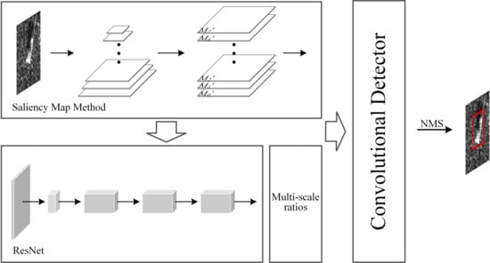
2. Methods
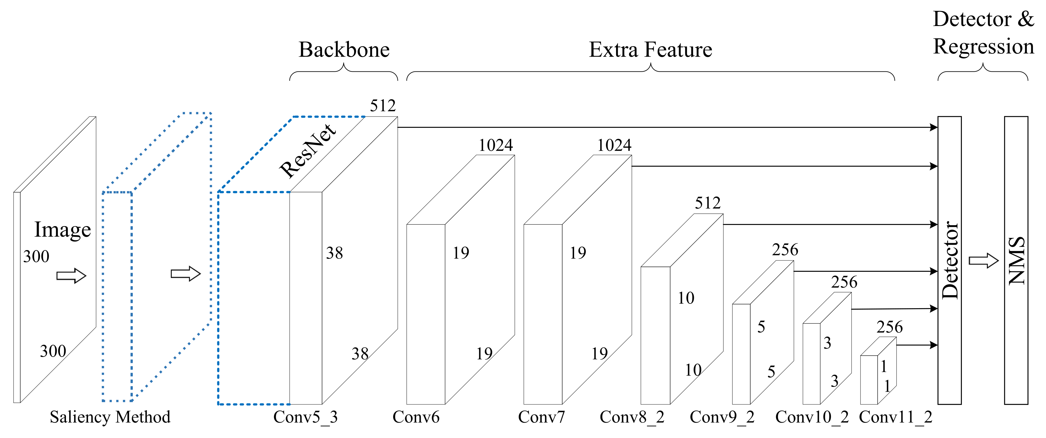
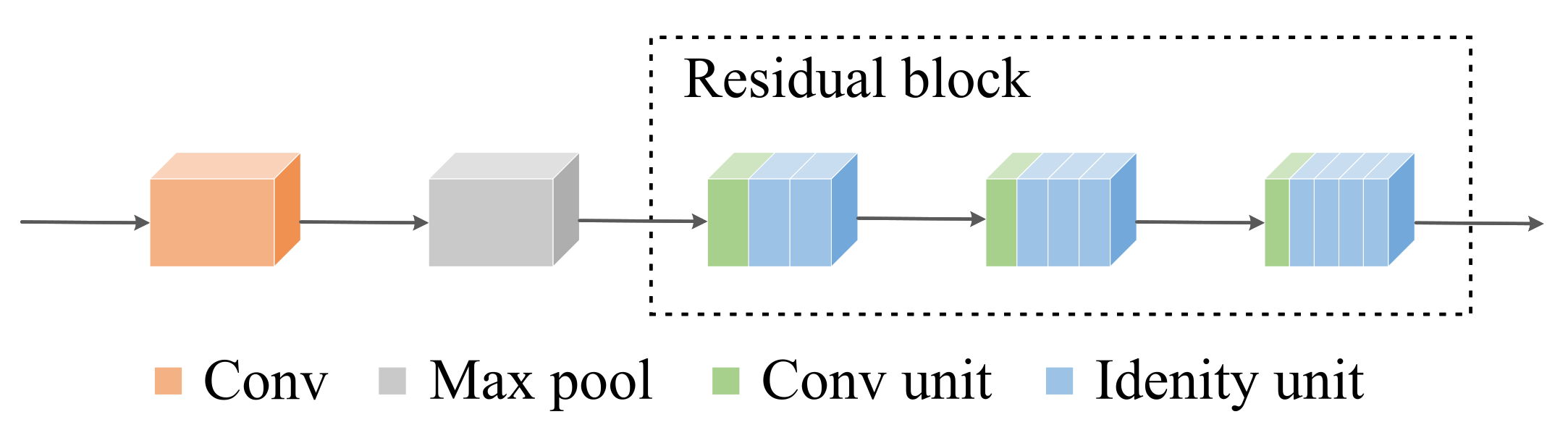
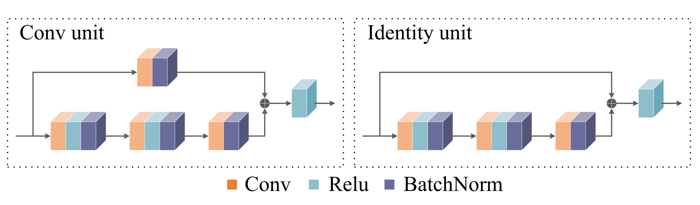
2.1. Feature Extraction
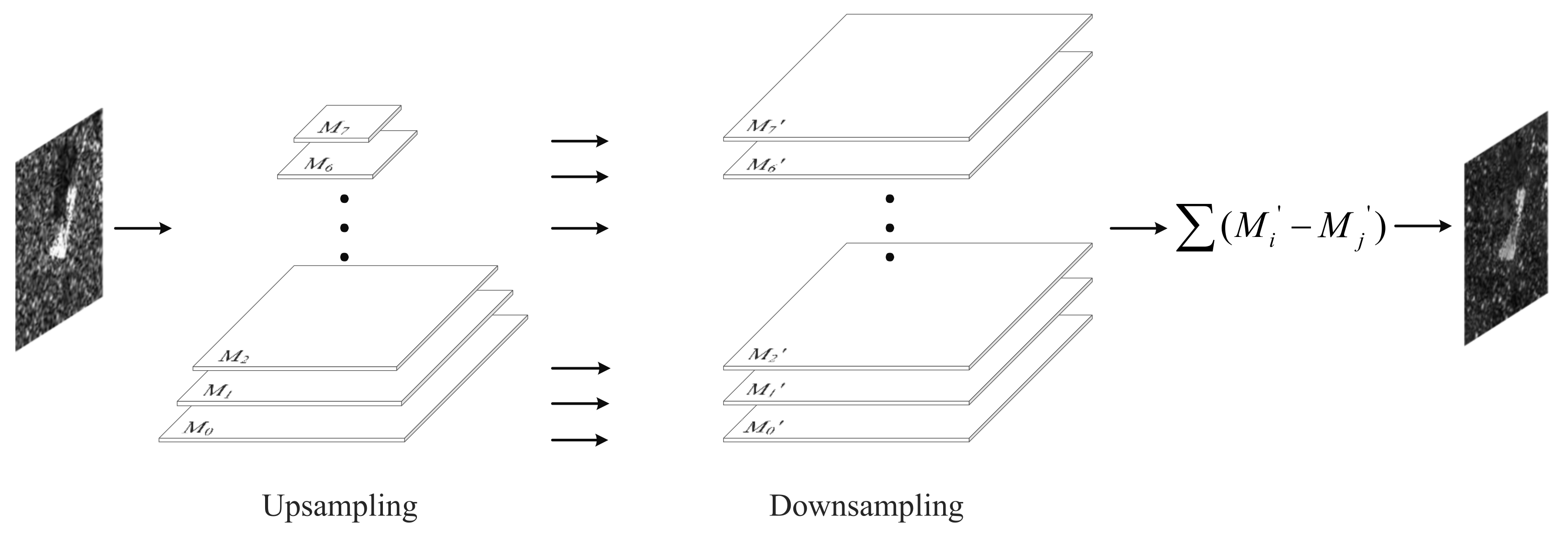
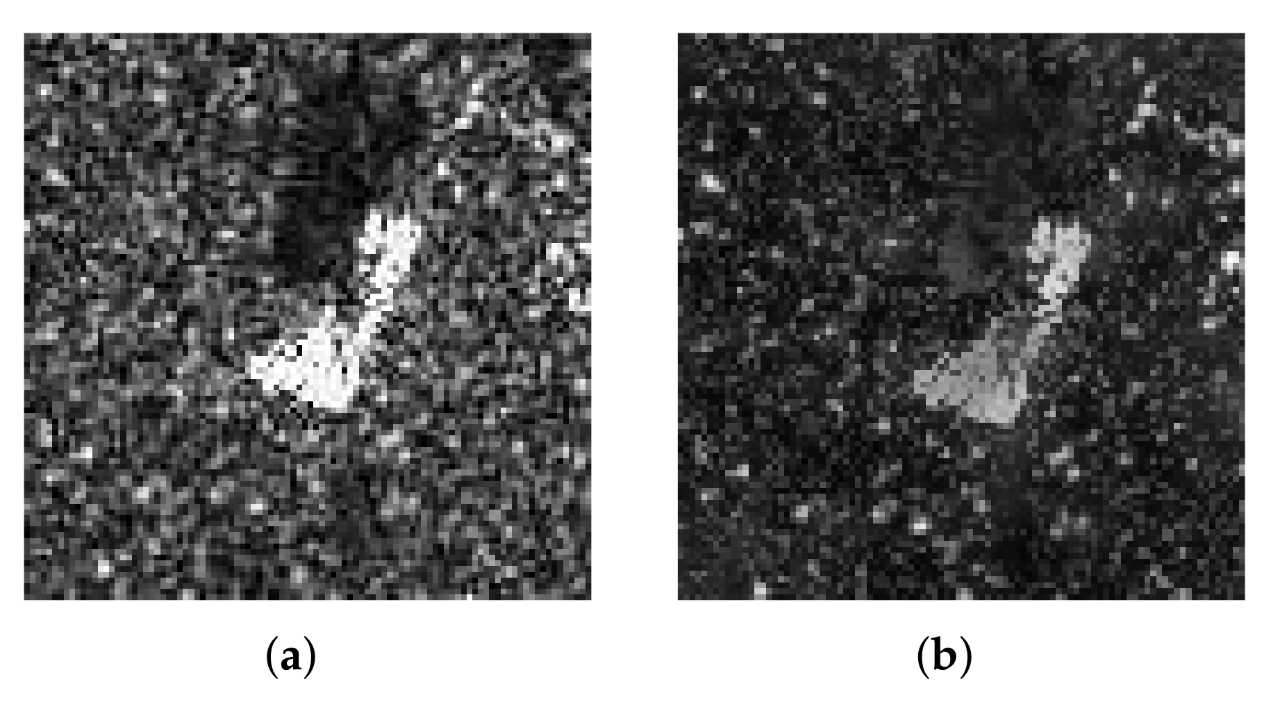
2.2. Small Sample Augmentation
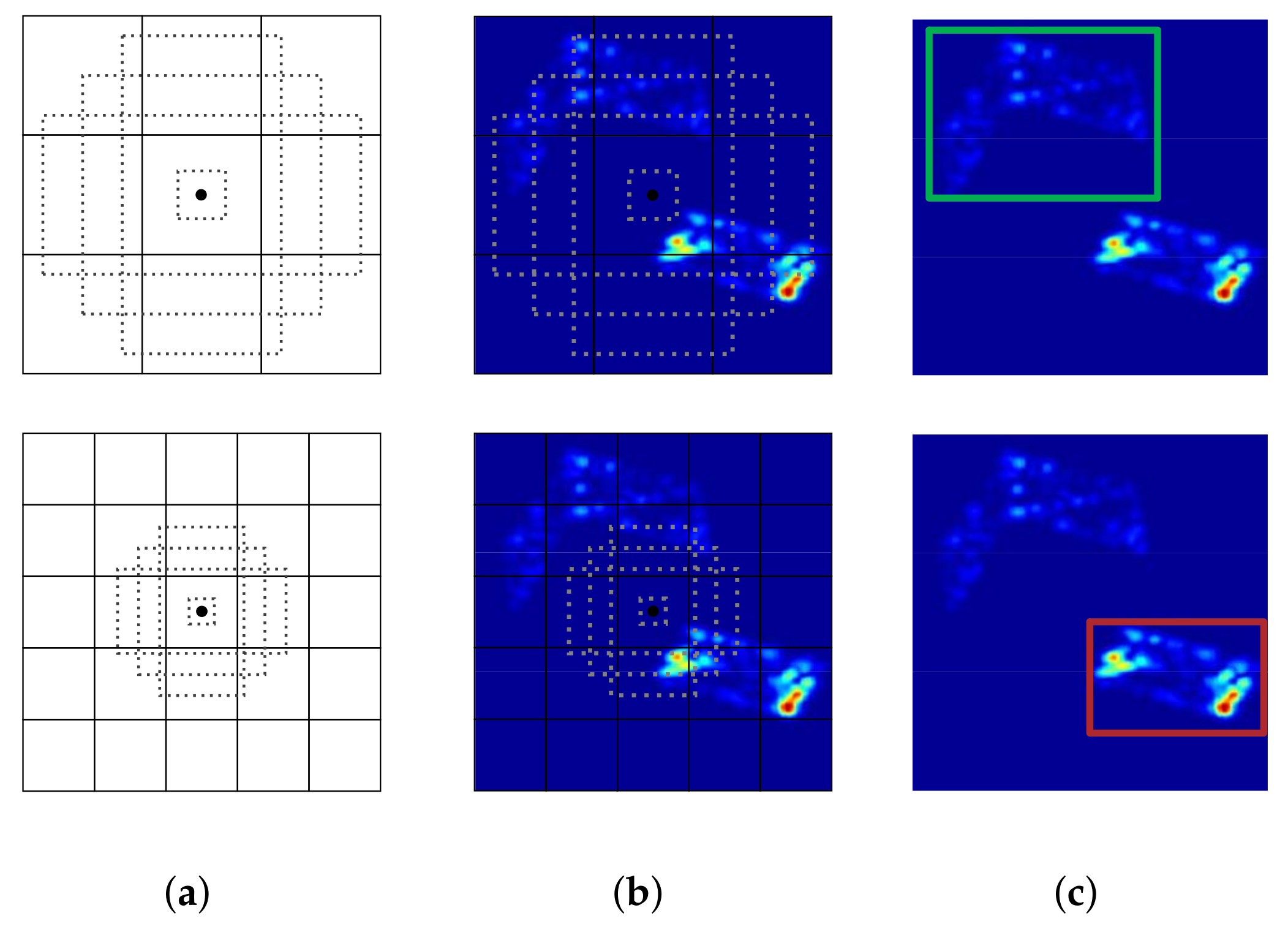
2.3. Aspect Ratios of Default Boxes
3. Experimental Results and Discussion
3.1. Datasets
3.2. Training Strategy
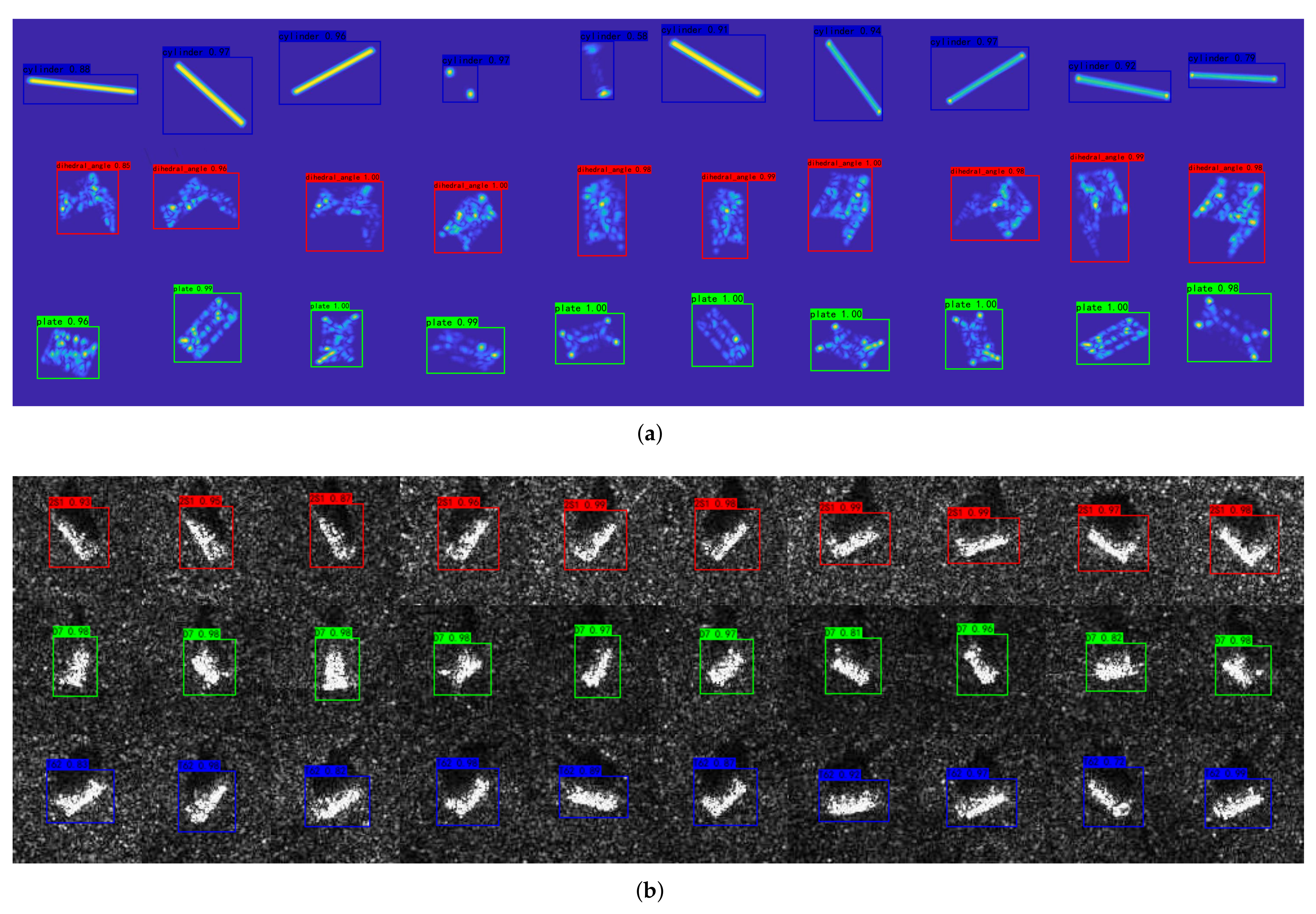
3.3. Experimental Results
3.4. Discussion
4. Conclusions
Author Contributions
Funding
Institutional Review Board Statement
Informed Consent Statement
Data Availability Statement
Conflicts of Interest
References
- Chen, J.; Zhang, J.; Jin, Y.; Yu, H.; Liang, B.; Yang, D.G. Real-Time Processing of Spaceborne SAR Data With Nonlinear Trajectory Based on Variable PRF. IEEE Trans. Geosci. Remote Sens. 2021, 60, 1–12. [Google Scholar] [CrossRef]
- Chen, J.; Xing, M.; Yu, H.; Liang, B.; Peng, J.; Sun, G.C. Motion Compensation/Autofocus in Airborne Synthetic Aperture Radar: A Review. IEEE Geosci. Remote Sens. Mag. 2021, 2–23. [Google Scholar] [CrossRef]
- Yang, T.; Li, S.; Xu, O.; Li, W.; Wang, Y. Three dimensional SAR imaging based on vortex electromagnetic waves. Remote Sens. Lett. 2018, 9, 343–352. [Google Scholar] [CrossRef]
- Kuo, J.M.; Chen, K.S. The application of wavelets correlator for ship wake detection in SAR images. IEEE Trans. Geosci. Remote Sens. 2003, 41, 1506–1511. [Google Scholar] [CrossRef]
- Kang, M.; Baek, J. SAR Image Change Detection via Multiple-Window Processing with Structural Similarity. Sensors 2021, 21, 6645. [Google Scholar] [CrossRef]
- Gao, Y.; Gao, F.; Dong, J.; Wang, S. Change Detection From Synthetic Aperture Radar Images Based on Channel Weighting-Based Deep Cascade Network. IEEE J. Sel. Top. Appl. Earth Obs. Remote Sens. 2019, 12, 4517–4529. [Google Scholar] [CrossRef]
- Joshi, S.K.; Baumgartner, S.V.; da Silva, A.B.C.; Krieger, G. Range-Doppler Based CFAR Ship Detection with Automatic Training Data Selection. Remote Sens. 2019, 11, 1270. [Google Scholar] [CrossRef] [Green Version]
- Huang, Y.; Liu, F. Detecting Cars in VHR SAR Images via Semantic CFAR Algorithm. IEEE Geosci. Remote Sens. Lett. 2016, 13, 801–805. [Google Scholar] [CrossRef]
- Fan, J.; Tomas, A. Target Reconstruction Based on Attributed Scattering Centers with Application to Robust SAR ATR. Remote Sens. 2018, 10, 655. [Google Scholar] [CrossRef] [Green Version]
- Zhu, J.; Qiu, X.; Pan, Z.; Zhang, Y.; Lei, B. Projection Shape Template-Based Ship Target Recognition in TerraSAR-X Images. IEEE Geosci. Remote Sens. Lett. 2017, 14, 222–226. [Google Scholar] [CrossRef]
- Girshick, R.; Donahue, J.; Darrell, T.; Malik, J. Rich feature hierarchies for accurate object detection and semantic segmentation. In Proceedings of the 2014 IEEE Conference on Computer Vision and Pattern Recognition, Columbus, OH, USA, 23–28 June 2014. [Google Scholar] [CrossRef] [Green Version]
- Girshick, R. Fast r-cnn. In Proceedings of the IEEE International Conference on Computer Vision, Santiago, Chile, 7–13 December 2015; pp. 1440–1448. [Google Scholar]
- Ren, S.; He, K.; Girshick, R.; Sun, J. Faster R-CNN: Towards Real-Time Object Detection with Region Proposal Networks. IEEE Trans. Pattern Anal. Mach. Intell. 2017, 39, 1137–1149. [Google Scholar] [CrossRef] [Green Version]
- Dai, J.; Li, Y.; He, K.; Sun, J. R-fcn: Object detection via region-based fully convolutional networks. In Proceedings of the Advances in Neural Information Processing Systems, Barcelona, Spain, 5–10 December 2016; pp. 379–387. [Google Scholar]
- Liu, W.; Anguelov, D.; Erhan, D.; Szegedy, C.; Reed, S.; Fu, C.Y.; Berg, A.C. Ssd: Single shot multibox detector. In Proceedings of the European Conference on Computer Vision, Amsterdam, The Netherlands, 8–16 October 2016; pp. 21–37. [Google Scholar]
- Redmon, J.; Divvala, S.; Girshick, R.; Farhadi, A. You only look once: Unified, real-time object detection. In Proceedings of the 2016 IEEE Conference on Computer Vision and Pattern Recognition (CVPR), Las Vegas, NV, USA, 27–30 June 2016. [Google Scholar] [CrossRef] [Green Version]
- Redmon, J.; Farhadi, A. YOLO9000: Better, faster, stronger. In Proceedings of the 2017 IEEE Conference on Computer Vision and Pattern Recognition (CVPR), Honolulu, HI, USA, 21–26 July 2017. [Google Scholar] [CrossRef] [Green Version]
- Redmon, J.; Farhadi, A. Yolov3: An incremental improvement. arXiv 2018, arXiv:1804.02767. [Google Scholar]
- Bochkovskiy, A.; Wang, C.Y.; Liao, H.Y.M. Yolov4: Optimal speed and accuracy of object detection. arXiv 2020, arXiv:2004.10934. [Google Scholar]
- Wang, Y.; Wang, C.; Zhang, H.; Dong, Y.; Wei, S. Automatic Ship Detection Based on RetinaNet Using Multi-Resolution Gaofen-3 Imagery. Remote Sens. 2019, 11, 531. [Google Scholar] [CrossRef] [Green Version]
- Ding, J.; Chen, B.; Liu, H.; Huang, M. Convolutional Neural Network with Data Augmentation for SAR Target Recognition. IEEE Geosci. Remote Sens. Lett. 2016, 13, 364–368. [Google Scholar] [CrossRef]
- Gao, F.; Shi, W.; Wang, J.; Yang, E.; Zhou, H. Enhanced Feature Extraction for Ship Detection from Multi-Resolution and Multi-Scene Synthetic Aperture Radar (SAR) Images. Remote Sens. 2019, 11, 2694. [Google Scholar] [CrossRef] [Green Version]
- Lin, Z.; Ji, K.; Kang, M.; Leng, X.; Zou, H. Deep Convolutional Highway Unit Network for SAR Target Classification with Limited Labeled Training Data. IEEE Geosci. Remote Sens. Lett. 2017, 14, 1091–1095. [Google Scholar] [CrossRef]
- He, Z.; Xiao, H.; Tian, Z. Multi-View Tensor Sparse Representation Model for SAR Target Recognition. IEEE Access 2019, 7, 48256–48265. [Google Scholar] [CrossRef]
- Wang, J.; Zheng, T.; Lei, P.; Bai, X. A Hierarchical Convolution Neural Network (CNN)-Based Ship Target Detection Method in Spaceborne SAR Imagery. Remote Sens. 2019, 11, 620. [Google Scholar] [CrossRef] [Green Version]
- Wang, Z.; Du, L.; Mao, J.; Liu, B.; Yang, D. SAR Target Detection Based on SSD With Data Augmentation and Transfer Learning. IEEE Geosci. Remote Sens. Lett. 2019, 16, 150–154. [Google Scholar] [CrossRef]
- Zhang, X.; Liu, G.; Zhang, C.; Atkinson, P.M.; Tan, X.; Jian, X.; Zhou, X.; Li, Y. Two-Phase Object-Based Deep Learning for Multi-Temporal SAR Image Change Detection. Remote Sens. 2020, 12, 548. [Google Scholar] [CrossRef] [Green Version]
- Chen, H.; Shi, Z. A Spatial-Temporal Attention-Based Method and a New Dataset for Remote Sensing Image Change Detection. Remote Sens. 2020, 12, 1662. [Google Scholar] [CrossRef]
- He, K.; Zhang, X.; Ren, S.; Sun, J. Deep residual learning for image recognition. In Proceedings of the 2016 IEEE Conference on Computer Vision and Pattern Recognition (CVPR), Las Vegas, NV, USA, 27–30 June 2016. [Google Scholar] [CrossRef] [Green Version]


| Layer Name | Parameters | Output Feature Size |
|---|---|---|
| Convolutional layer | 7 × 7 Conv, stride 2 | 300 × 300 × 64 |
| Pooling layer | 3 × 3 Max pool, stride 2 | 150 × 150 × 64 |
| Residual block 1 | × 3 | 150 × 150 × 256 |
| Residual block 2 | × 4 | 75 × 75 × 512 |
| Residual block 3 | × 6 | 38 × 38 × 512 |
| Dataset | Training Set | Testing Set | |
|---|---|---|---|
| Initial Quantity | After Augmentation | ||
| GO | 131 | 3930 | 230 |
| MSTAR | 821 | 1642 | 897 |
| AP (%) | GO | MSTAR | ||||||
|---|---|---|---|---|---|---|---|---|
| mAP (%) | Dihedral Angle | Surface Plate | Cylinder | mAP (%) | 2S1 | D7 | t62 | |
| Faster R-CNN | 96.73 | 98.54 | 98.57 | 93.08 | 95.98 | 94.06 | 99.78 | 94.10 |
| YOLOv3 | 96.87 | 98.89 | 96.50 | 95.21 | 96.39 | 92.93 | 99.76 | 96.47 |
| SSD | 94.63 | 98.09 | 95.10 | 91.61 | 96.01 | 96.57 | 98.49 | 92.97 |
| Ours | 99.50 | 99.96 | 98.88 | 99.66 | 98.40 | 98.62 | 99.83 | 96.75 |
| Backbone | Layers | Memory Size (MB) | Input Size |
|---|---|---|---|
| VGG16 | 13 | 56.13 | 300 × 300 × 3 |
| residual network | 40 | 26.20 | 600 × 600 × 3 |
Publisher’s Note: MDPI stays neutral with regard to jurisdictional claims in published maps and institutional affiliations. |
© 2022 by the authors. Licensee MDPI, Basel, Switzerland. This article is an open access article distributed under the terms and conditions of the Creative Commons Attribution (CC BY) license (https://creativecommons.org/licenses/by/4.0/).
Share and Cite
Zhou, F.; He, F.; Gui, C.; Dong, Z.; Xing, M. SAR Target Detection Based on Improved SSD with Saliency Map and Residual Network. Remote Sens. 2022, 14, 180. https://doi.org/10.3390/rs14010180
Zhou F, He F, Gui C, Dong Z, Xing M. SAR Target Detection Based on Improved SSD with Saliency Map and Residual Network. Remote Sensing. 2022; 14(1):180. https://doi.org/10.3390/rs14010180
Chicago/Turabian StyleZhou, Fang, Fengjie He, Changchun Gui, Zhangyu Dong, and Mengdao Xing. 2022. "SAR Target Detection Based on Improved SSD with Saliency Map and Residual Network" Remote Sensing 14, no. 1: 180. https://doi.org/10.3390/rs14010180
APA StyleZhou, F., He, F., Gui, C., Dong, Z., & Xing, M. (2022). SAR Target Detection Based on Improved SSD with Saliency Map and Residual Network. Remote Sensing, 14(1), 180. https://doi.org/10.3390/rs14010180