
A Lightweight Convolutional Neural Network Based on Group-Wise Hybrid Attention for Remote Sensing Scene Classification


Abstract
:
1. Introduction
- (1)
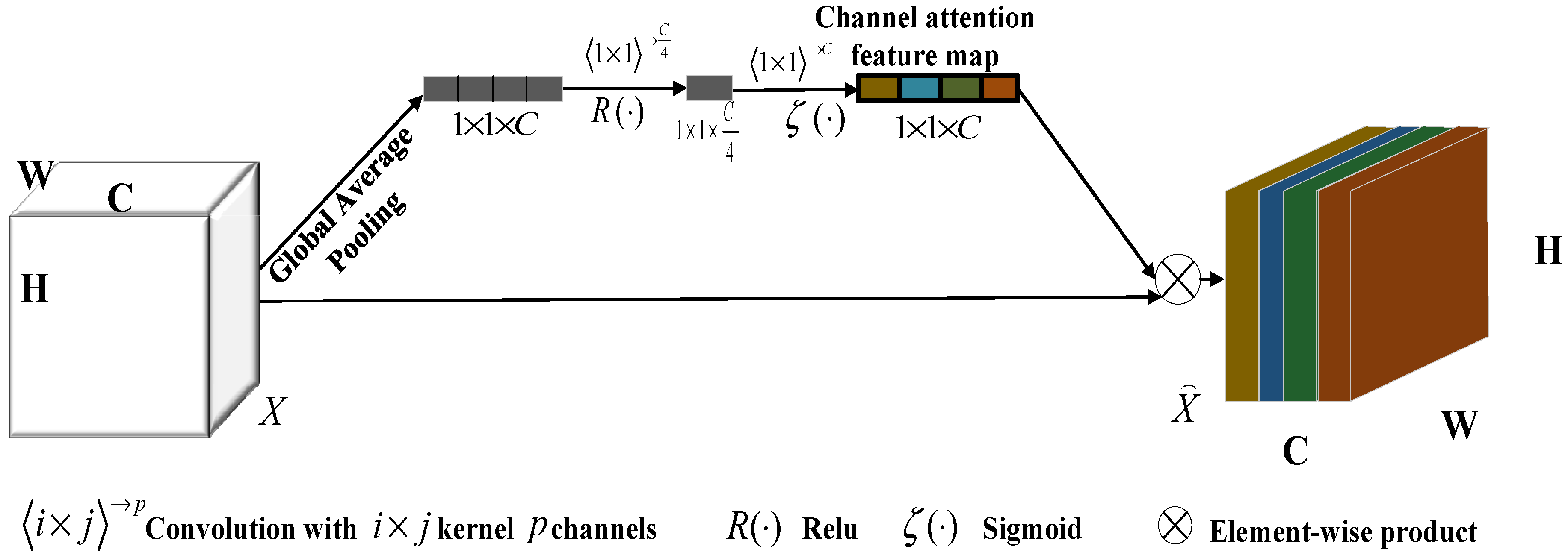
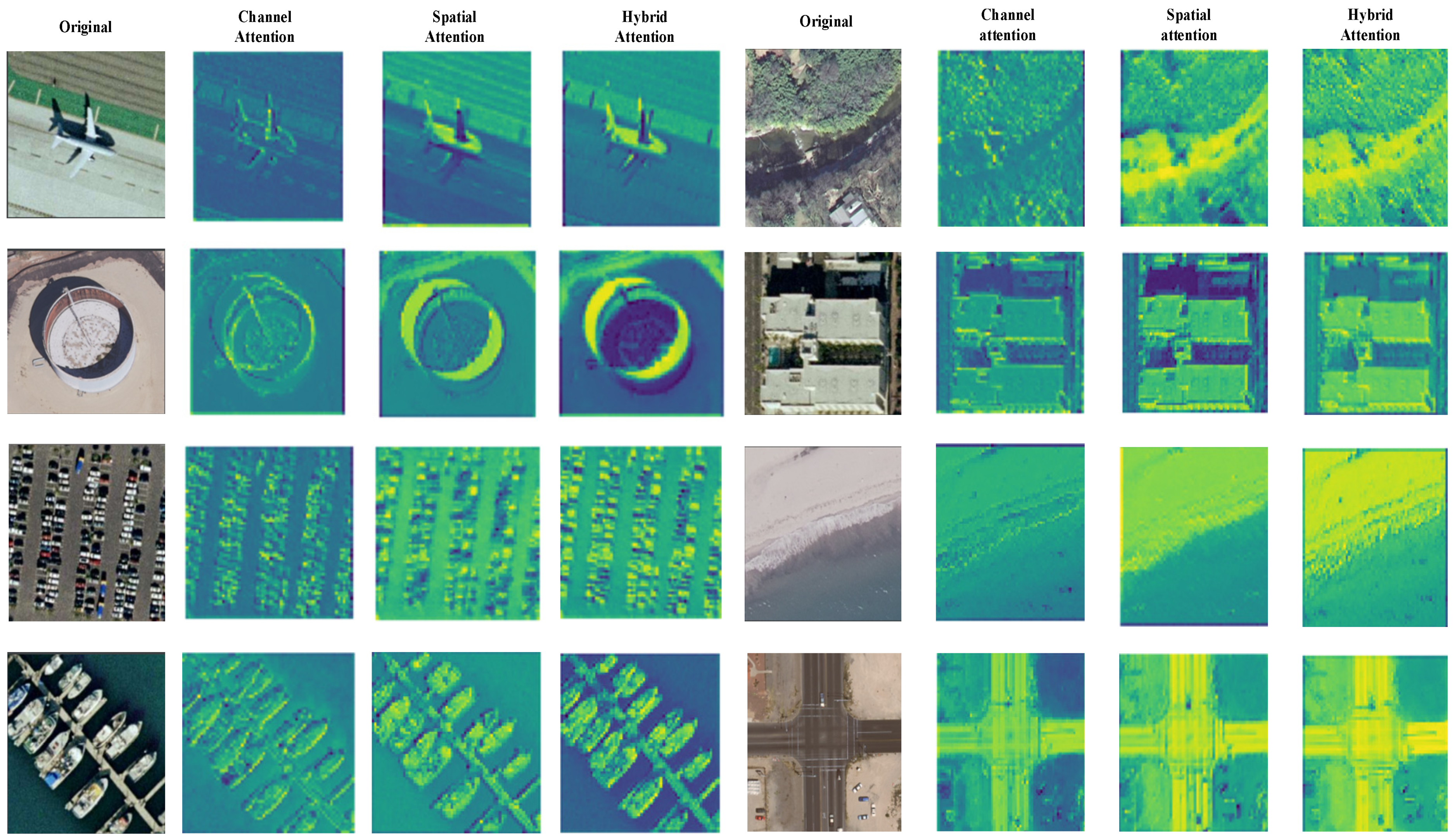
- Based on the SE module, we propose a channel attention module which is more suitable for remote sensing scene image classification. In the proposed method, the channel compression ratio is set to 1/4, and a 1 × 1 convolution kernel is adopted instead of a fully connected layer. The 1 × 1 convolution does not destroy the spatial structure of the features, and the size of the input features can be arbitrary.
- (2)
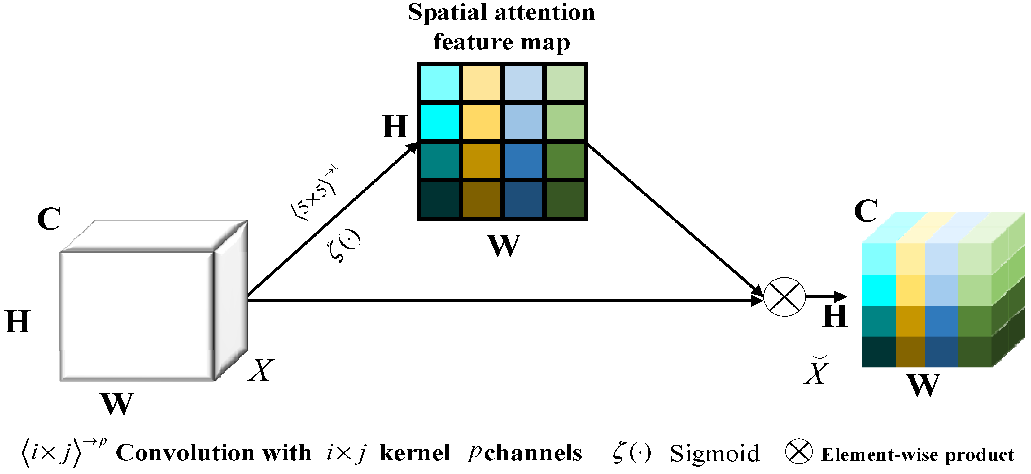
- We propose a spatial attention module with a simpler implementation process. Channels are compressed using a 5 × 5 × 1 convolution kernel directly, and spatial attention features are obtained using the Sigmoid activation function. The convolution kernel of 5 × 5 is helpful in providing a large receptive field, which can extract more spatial features.
- (3)
- A hybrid attention model is constructed by combining channel attention and spatial attention in parallel, which has higher activation and can learn more meaningful features.
- (4)
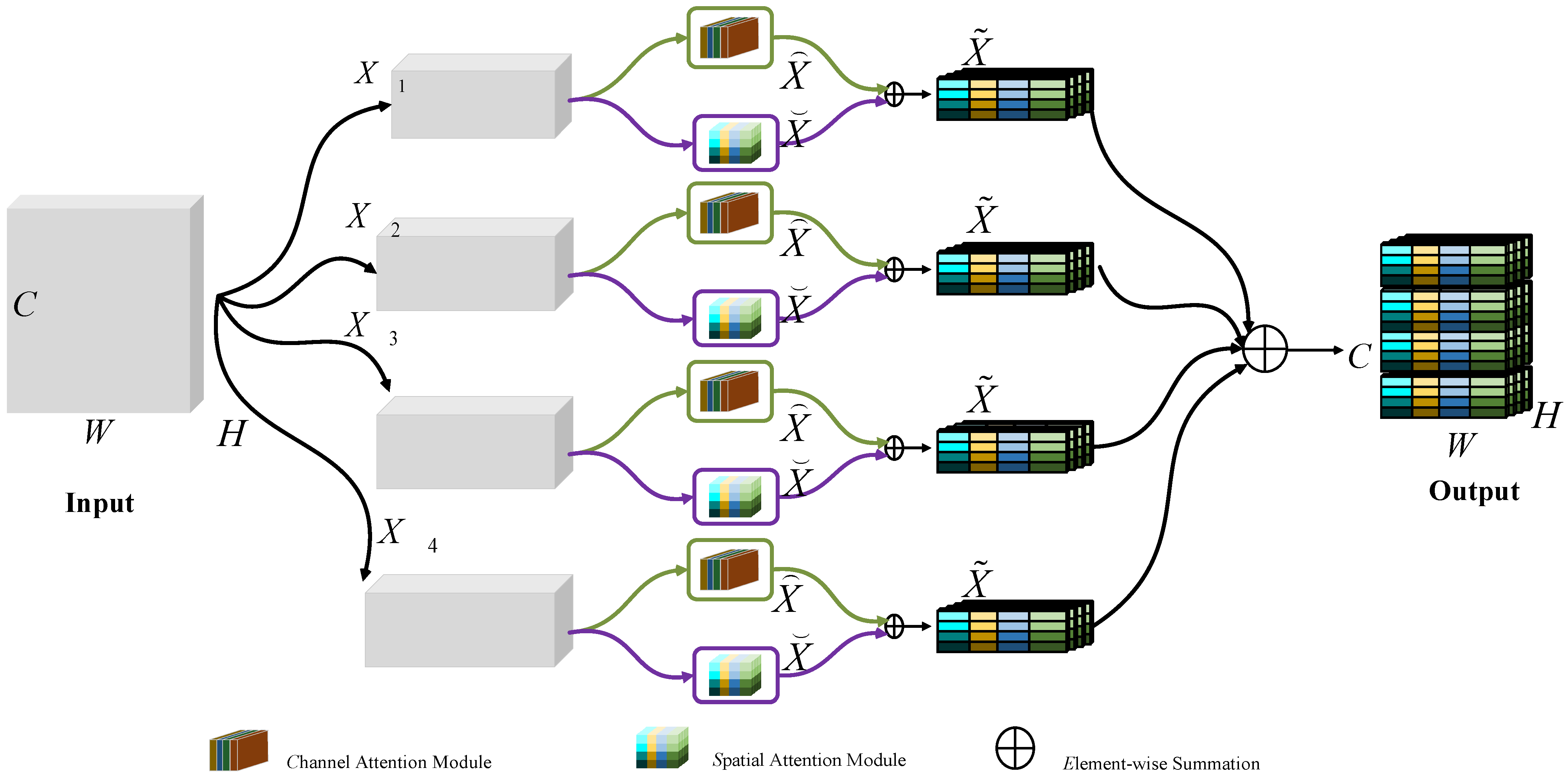
- To alleviate the problem that the introduction of attention leads to an increased number of parameters, we further propose a group-wise hybrid attention module. This module first divides input features into four groups in the channel dimension, then introduces hybrid attention to each group. Each group is recalibrated separately with spatial attention and channel attention and, finally, the rescaled features are fused in the channel dimension. Moreover, a lightweight convolutional neural network is constructed based on group-wise hybrid attention (LCNN-GWHA), which is shown to be an effective method for remote sensing scene image classification.
2. Methods
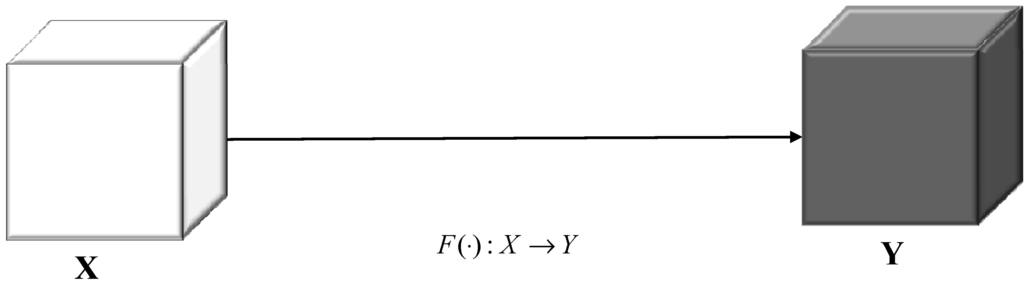
2.1. Traditional Convolution Process
2.2. Channel Attention
2.3. Spatial Attention
2.4. Group-Wise Hybrid Attention
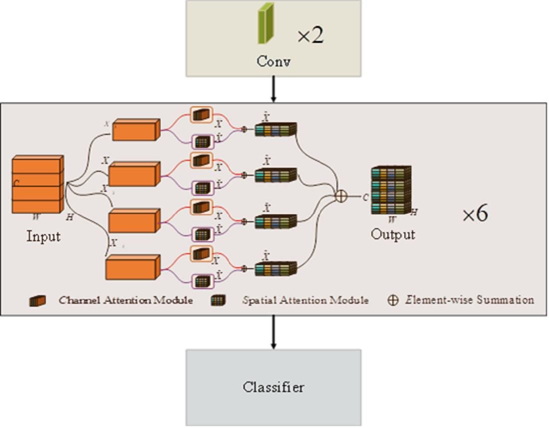
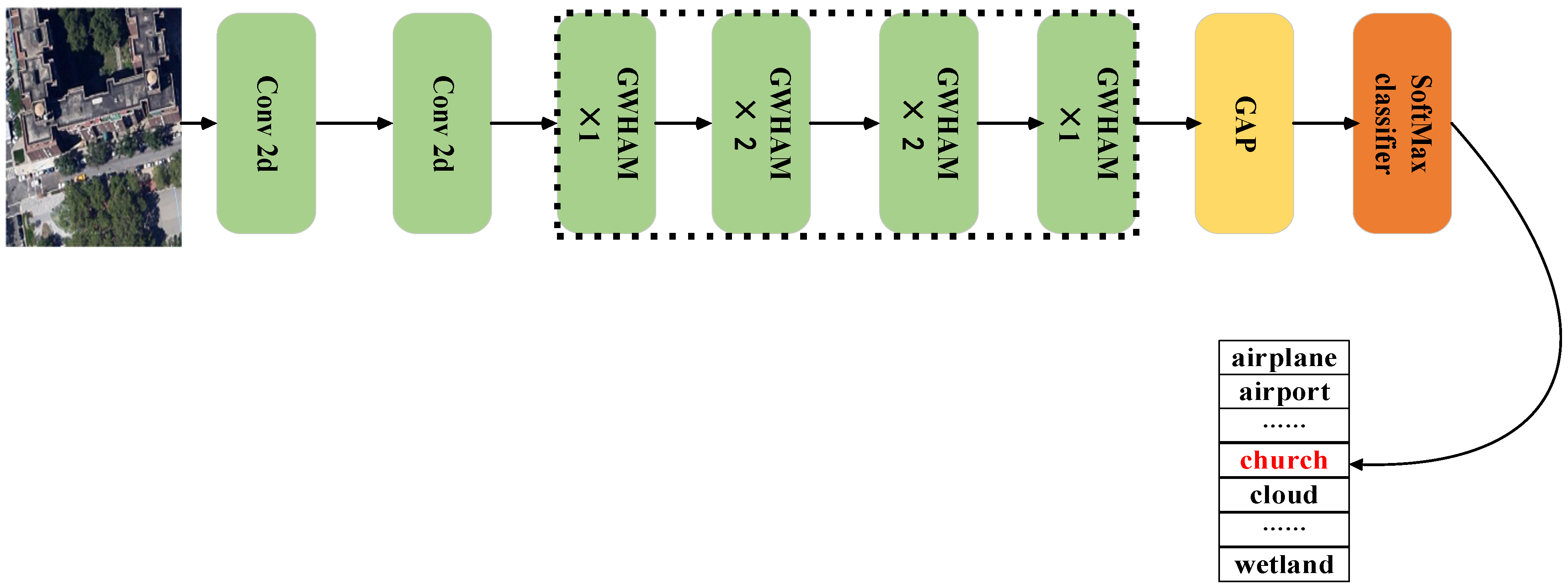
2.5. Lightweight Convolution Neural Network Based on Group-Wise Hybrid Attention (LCNN-GWHA)
3. Experiments
3.1. Dataset Settings
3.2. Setting of the Experiments
3.3. Performance of the Proposed Model
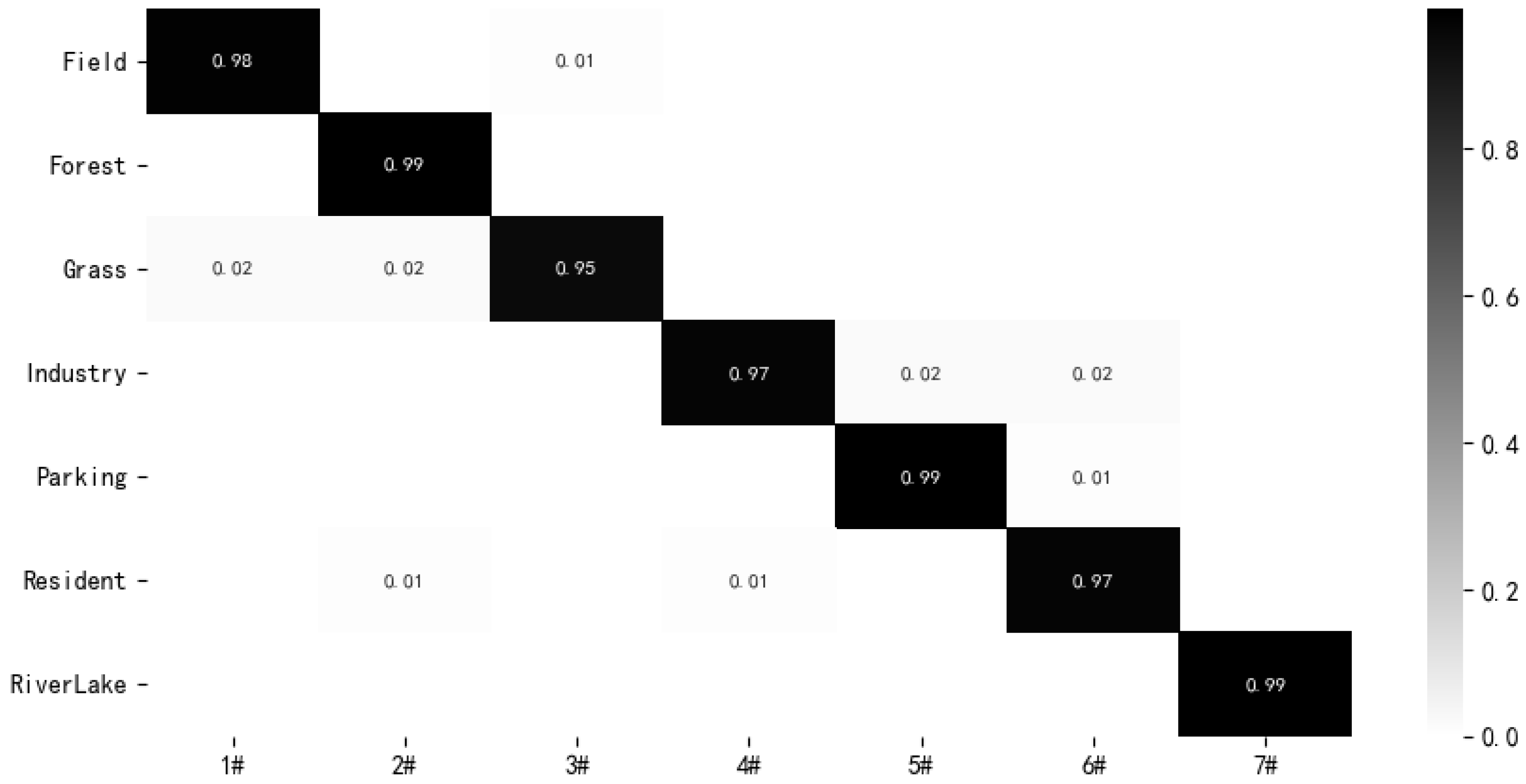
3.3.1. Experimental Results of the RSSCN7 Dataset
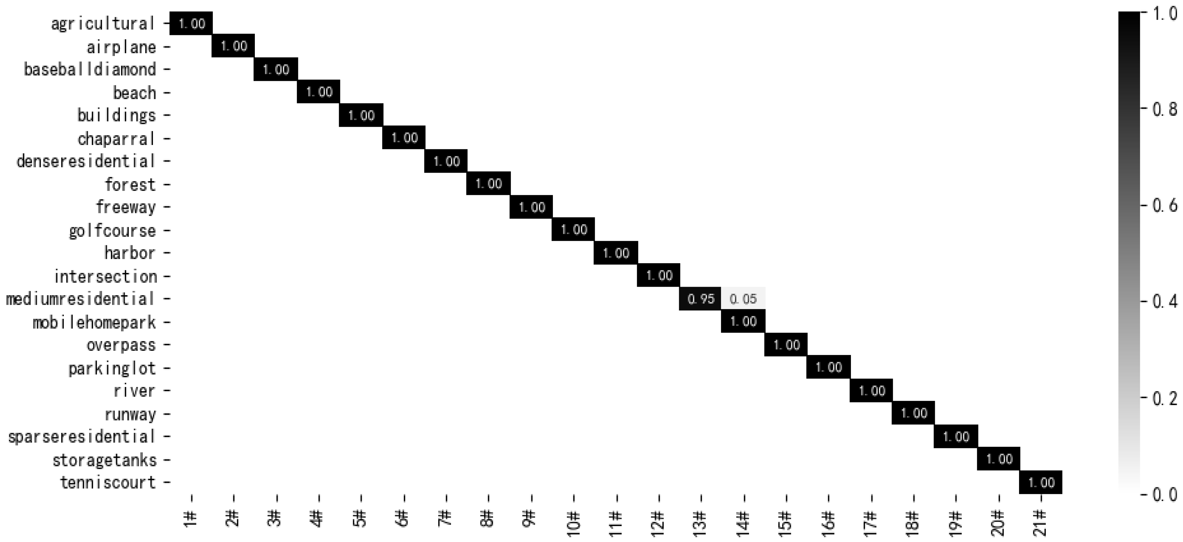
3.3.2. Experimental Results of the UCM21 Dataset
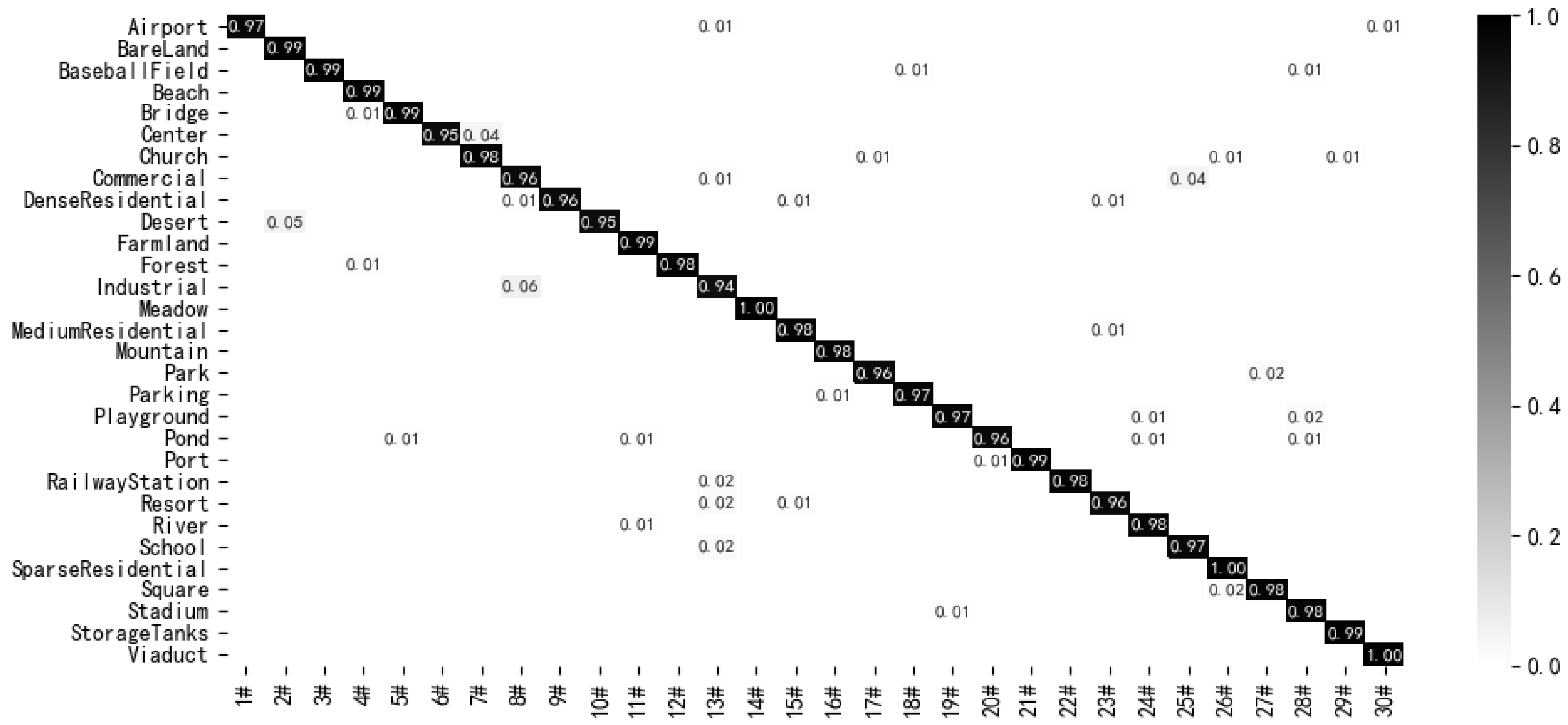
3.3.3. Experimental Results on the AID Dataset
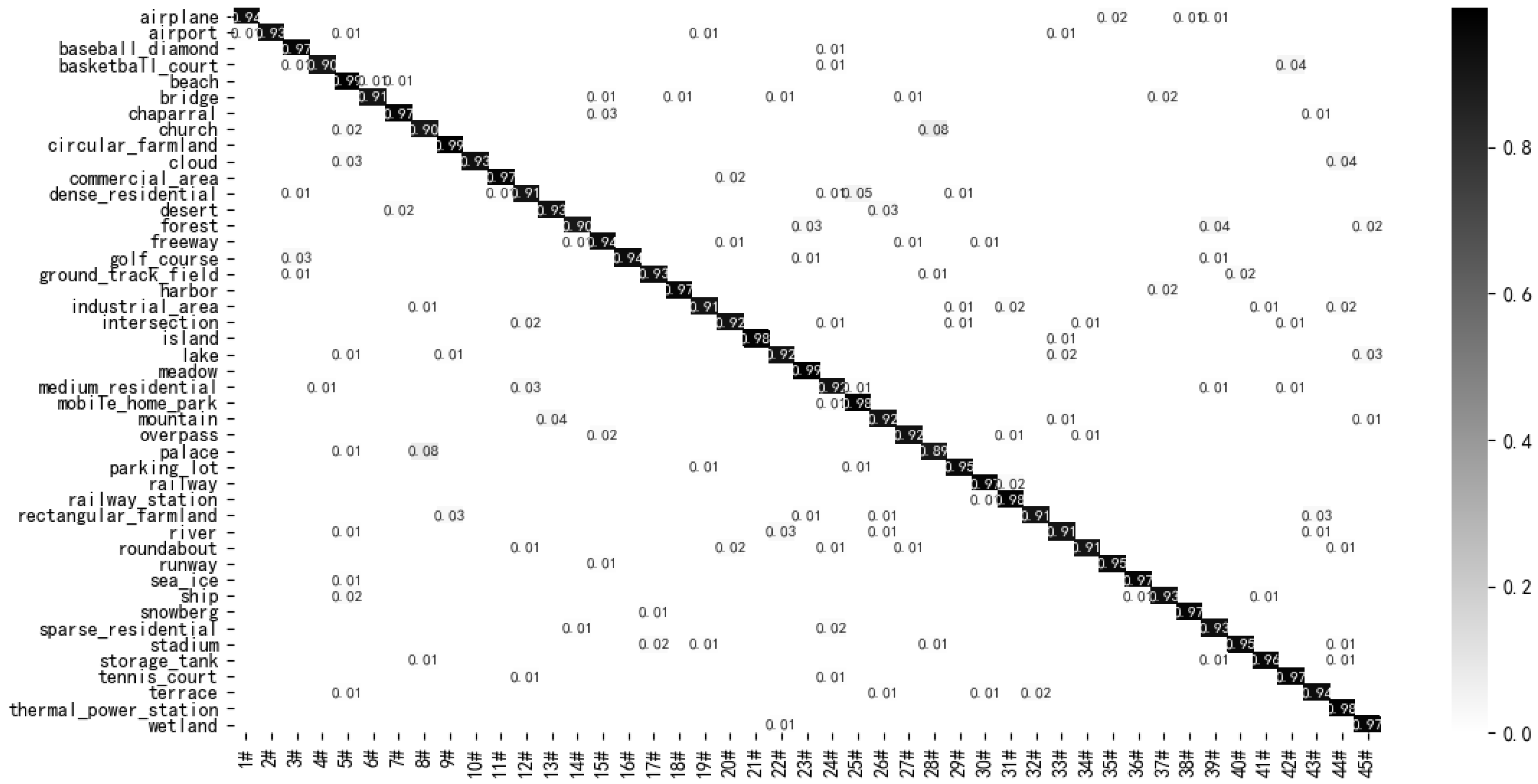
3.3.4. Experimental Results on the NWPU45 Dataset
3.4. Speed Comparison of Models
3.5. Comparison of Computational Complexity of Models
4. Discussion
5. Conclusions
Author Contributions
Funding
Institutional Review Board Statement
Informed Consent Statement
Data Availability Statement
Acknowledgments
Conflicts of Interest
References
- Krizhevsky, A.; Sutskever, I.; Hinton, G.E. ImageNet classification with deep convolutional neural networks. Adv. Neural Inf. Process. Syst. 2012, 25, 1097–1105. [Google Scholar] [CrossRef]
- Toshev, A.; Szegedy, C. DeepPose: Human Pose Estimation via Deep Neural Networks. In Proceedings of the IEEE Computer Society Conference on Computer Vision and Pattern Recognition, Columbus, OH, USA, 23–28 June 2014; pp. 1653–1660. [Google Scholar]
- Long, J.; Shelhamer, E.; Darrell, T. Fully convolutional networks for semantic segmentation. In Proceedings of the IEEE Conference on Computer Vision and Pattern Recognition, Columbus, OH, USA, June 2015; pp. 3431–3440. [Google Scholar]
- Ren, S.; He, K.; Girshick, R.; Sun, J. Faster R-CNN: Towards real-time object detection with region proposal networks. Adv. Neural Inf. Process. Syst. 2015, 28, 91–99. [Google Scholar] [CrossRef] [PubMed] [Green Version]
- Zheng, X.; Chen, X.; Lu, X.; Sun, B. Unsupervised Change Detection by Cross-Resolution Difference Learning. IEEE Trans. Geosci. Remote. Sens. 2021, 18, 1–16. [Google Scholar] [CrossRef]
- Zheng, X.; Wang, B.; Du, X.; Lu, X. Mutual Attention Inception Network for Remote Sensing Visual Question Answering. IEEE Trans. Geosci. Remote. Sens. 2021, 18, 1–14. [Google Scholar] [CrossRef]
- Luo, F.; Zou, Z.; Liu, J.; Lin, Z. Dimensionality reduction and classification of hyperspectral image via multi-structure unified discriminative embedding. IEEE Trans. Geosci. Remote Sens. 2021, 18, 1. [Google Scholar] [CrossRef]
- He, K.; Zhang, X.; Ren, S.; Sun, J. Deep Residual Learning for Image Recognition. In Proceedings of the IEEE Conference on Computer Vision and Pattern Recognition, Las Vegas, NV, USA, 27–30 June 2016; pp. 770–778. [Google Scholar]
- Luo, F.; Huang, H.; Ma, Z.; Liu, J. Semi-supervised Sparse Manifold Discriminative Analysis for Feature Extraction of Hyperspectral Images. IEEE Trans. Geosci. Remote Sens. 2016, 54, 6197–6221. [Google Scholar] [CrossRef]
- Luo, F.; Zhang, L.; Zhou, X.; Guo, T.; Cheng, Y.; Yin, T. Sparse-Adaptive Hypergraph Discriminant Analysis for Hyperspectral Image Classification. IEEE Geosci. Remote Sens. Lett. 2020, 17, 1082–1086. [Google Scholar] [CrossRef]
- Zheng, X.; Gong, T.; Li, X.; Lu, X. Generalized Scene Classification From Small-Scale Datasets With Multitask Learning. IEEE Trans. Geosci. Remote Sens. 2021, 18, 1–11. [Google Scholar] [CrossRef]
- Simonyan, K.; Zisserman, A. Very deep convolutional networks for large-scale image recognition. arXiv 2014, arXiv:1409.1556. [Google Scholar]
- He, K.; Zhang, X.; Ren, S.; Sun, J. Identity Mappings in Deep Residual Networks. In Proceedings of the 14th European Conference on Computer Vision, Amsterdam, The Netherlands, 11–14 October 2016; pp. 630–645. [Google Scholar] [CrossRef] [Green Version]
- Ioffe, S.; Szegedy, C. Batch normalization: Accelerating deep network training by reducing internal covariate shift. arXiv 2015, arXiv:1502.03167. [Google Scholar]
- Carreira, J.; Madeira, H.; Silva, J.G. Xception: A technique for the experimental evaluation of dependability in modern computers. IEEE Trans. Softw. Eng. 1998, 24, 125–136. [Google Scholar] [CrossRef] [Green Version]
- Howard, A.G.; Zhu, M.; Chen, B.; Kalenichenko, D.; Wang, W.; Weyand, M.; Andreetto, M.; Adam, H. Mobilenets: Efficient convolutional neural networks for mobile vision applications. arXiv 2017, arXiv:1704.04861. [Google Scholar]
- Sandler, M.; Howard, A.; Zhu, M.; Zhmoginov, A.; Chen, L. MobileNetV2: Inverted residuals and linear bottlenecks. In Proceedings of the IEEE/CVF Conference on Computer Vision and Pattern Recognition (CVPR), Salt Lake City, UT, USA, 18–23 June 2018; pp. 4510–4520. [Google Scholar] [CrossRef] [Green Version]
- Xie, S.N.; Girshick, R.; Dollar, P.; Tu, Z.W.; He, K.M. Aggregated Residual Transformations for Deep Neural Networks. In Proceedings of the IEEE Conference on Computer Vision and Pattern Recognition (CVPR), Honolulu, HI, USA, 21–26 July 2017; pp. 5987–5995. [Google Scholar] [CrossRef] [Green Version]
- Zhang, X.; Zhou, X.; Lin, M.; Sun, J. ShuffleNet: An Extremely Efficient Convolutional Neural Network for Mobile Devices. In Proceedings of the 2018 IEEE/CVF Conference on Computer Vision and Pattern Recognition, Salt Lake City, UT, USA, 18–23 June 2018; p. 18326147. [Google Scholar]
- Ma, N.; Zhang, X.; Zheng, H.T.; Sun, J. Shufflflenet v2: Practical guidelines for efficient cnn architecture design. arXiv 2018, arXiv:1807.11164. [Google Scholar]
- Hu, J.; Shen, L.; Sun, G. Squeeze-and-Excitation Networks. In Proceedings of the IEEE Conference on Computer Vision and Pattern Recognition (CVPR), Salt Lake City, UT, USA, 18–23 June 2018; pp. 7132–7141. [Google Scholar]
- Li, X.; Wang, W.; Hu, X.; Yang, J. Selective kernel networks. In Proceedings of the 2019 IEEE/CVF Conference on Computer Vision and Pattern Recognition (CVPR), Long Beach, CA, USA, 15–20 June 2019; pp. 510–519. [Google Scholar]
- Woo, S.; Park, J.; Lee, J.; Kweon, I.S. CBAM: Convolutional Block Attention Module. In Proceedings of the 2018 European Conference on Computer Vision, Munich, Germany, 8–14 September 2018. [Google Scholar]
- Wang, Q.; Liu, S.; Chanussot, J.; Li, X. Scene Classification With Recurrent Attention of VHR Remote Sensing Images. IEEE Trans. Geosci. Remote Sens. 2019, 57, 1155–1167. [Google Scholar] [CrossRef]
- Tong, W.; Chen, W.; Han, W.; Li, X.; Wang, L. Channel-Attention-Based DenseNet Network for Remote Sensing Image Scene Classification. IEEE J. Sel. Top. Appl. Earth Obs. Remote Sens. 2020, 13, 4121–4132. [Google Scholar] [CrossRef]
- Yu, D.; Guo, H.; Xu, Q.; Lu, J.; Zhao, C.; Lin, Y. Hierarchical Attention and Bilinear Fusion for Remote Sensing Image Scene Classification. IEEE J. Sel. Top. Appl. Earth Obs. Remote Sens. 2020, 13, 6372–6383. [Google Scholar] [CrossRef]
- Alhichri, H.; Alswayed, A.S.; Bazi, Y.; Ammour, N.; Alajlan, N.A. Classification of Remote Sensing Images Using EfficientNet-B3 CNN Model With Attention. IEEE Access 2021, 9, 14078–14094. [Google Scholar] [CrossRef]
- Yang, Y.; Newsam, S. Bag-of-visual-words and spatial extensions for land-use classification. In Proceedings of the 18th SIGSPATIAL International Conference on Advances in Geographic Information Systems, San Jose, CA, USA, 3–5 November 2010; pp. 270–279. [Google Scholar]
- Zou, Q.; Ni, L.; Zhang, T.; Wang, Q. Deep Learning Based Feature Selection for Remote Sensing Scene Classification. IEEE Geosci. Remote Sens. Lett. 2015, 12, 2321–2325. [Google Scholar] [CrossRef]
- Xia, G.-S.; Hu, J.; Hu, F.; Shi, B.; Bai, X.; Zhong, Y.; Zhang, L.; Lu, X. AID: A Benchmark Data Set for Performance Evaluation of Aerial Scene Classification. IEEE Trans. Geosci. Remote Sens. 2017, 55, 3965–3981. [Google Scholar] [CrossRef] [Green Version]
- Cheng, G.; Han, J.; Lu, X. Remote Sensing Image Scene Classification: Benchmark and State of the Art. Proc. IEEE. 2017, 105, 1865–1883. [Google Scholar] [CrossRef] [Green Version]
- Li, B.; Su, W.; Wu, H.; Li, R.; Zhang, W.; Qin, W.; Zhang, S. Aggregated Deep Fisher Feature for VHR Remote Sensing Scene Classification. IEEE J. Sel. Top. Appl. Earth Obs. Remote Sens. 2019, 12, 3508–3523. [Google Scholar] [CrossRef]
- Liu, M.; Jiao, L.; Liu, X.; Li, L.; Liu, F.; Yang, S. C-CNN: Contourlet Convolutional Neural Networks. IEEE Trans. Neural Netw. Learn. Syst. 2021, 32, 2636–2649. [Google Scholar] [CrossRef] [PubMed]
- Zhang, B.; Zhang, Y.; Wang, S. A Lightweight and Discriminative Model for Remote Sensing Scene Classification With Multidilation Pooling Module. IEEE J. Sel. Top. Appl. Earth Obs. Remote Sens. 2019, 12, 2636–2653. [Google Scholar] [CrossRef]
- Zhao, F.; Mu, X.; Yang, Z.; Yi, Z. A novel two-stage scene classification model based on feature variable significance in high-resolution remote sensing. Geocarto Int. 2019, 35, 1603–1614. [Google Scholar] [CrossRef]
- Liu, Y.; Liu, Y.; Ding, L. Scene classification based on two-stage deep feature fusion. IEEE Geosci. Remote Sens. Lett. 2018, 15, 183–186. [Google Scholar] [CrossRef]
- Liu, B.-D.; Meng, J.; Xie, W.-Y.; Shao, S.; Li, Y.; Wang, Y. Weighted Spatial Pyramid Matching Collaborative Representation for Remote-Sensing-Image Scene Classification. Remote Sens. 2019, 11, 518. [Google Scholar] [CrossRef] [Green Version]
- Shi, C.; Wang, T.; Wang, L. Branch Feature Fusion Convolution Network for Remote Sensing Scene Classification. IEEE J. Sel. Top. Appl. Earth Obs. Remote Sens. 2020, 13, 5194–5210. [Google Scholar] [CrossRef]
- Zhang, W.; Tang, P.; Zhao, L. Remote sensing image scene classification using CNN-CapsNet. Remote Sens. 2019, 11, 494. [Google Scholar] [CrossRef] [Green Version]
- He, N.; Fang, L.; Li, S.; Plaza, A.; Plaza, J. Remote Sensing Scene Classification Using Multilayer Stacked Covariance Pooling. IEEE Trans. Geosci. Remote. Sens. 2018, 56, 6899–6910. [Google Scholar] [CrossRef]
- Sun, H.; Li, S.; Zheng, X.; Lu, X. Remote Sensing Scene Classification by Gated Bidirectional Network. IEEE Trans. Geosci. Remote Sens. 2020, 58, 82–96. [Google Scholar] [CrossRef]
- Lu, X.; Sun, H.; Zheng, X. A Feature Aggregation Convolutional Neural Network for Remote Sensing Scene Classification. IEEE Trans. Geosci. Remote Sens. 2019, 57, 7894–7906. [Google Scholar] [CrossRef]
- He, N.; Fang, L.; Li, S.; Plaza, J.; Plaza, A. Skip-Connected Covariance Network for Remote Sensing Scene Classification. IEEE Trans. Neural Netw. Learn. Syst. 2019, 31, 1461–1474. [Google Scholar] [CrossRef] [PubMed] [Green Version]
- Cheng, G.; Yang, C.; Yao, X.; Guo, L.; Han, J. When Deep Learning Meets Metric Learning: Remote Sensing Image Scene Classification via Learning Discriminative CNNs. IEEE Trans. Geosci. Remote Sens. 2018, 56, 2811–2821. [Google Scholar] [CrossRef]
- Boualleg, Y.; Farah, M.; Farah, I.R. Remote Sensing Scene Classification Using Convolutional Features and Deep Forest Classifier. IEEE Geosci. Remote Sens. Lett. 2019, 16, 1944–1948. [Google Scholar] [CrossRef]
- Xie, J.; He, N.; Fang, L.; Plaza, A. Scale-Free Convolutional Neural Network for Remote Sensing Scene Classification. IEEE Trans. Geosci. Remote Sens. 2019, 57, 6916–6928. [Google Scholar] [CrossRef]
- Li, J.; Lin, D.; Wang, Y.; Xu, G.; Zhang, Y.; Ding, C.; Zhou, Y. Deep Discriminative Representation Learning with Attention Map for Scene Classification. Remote Sens. 2020, 12, 1366. [Google Scholar] [CrossRef]
- Yan, P.; He, F.; Yang, Y.; Hu, F. Semi-Supervised Representation Learning for Remote Sensing Image Classification Based on Generative Adversarial Networks. IEEE Access 2020, 8, 54135–54144. [Google Scholar] [CrossRef]
- Wang, C.; Lin, W.; Tang, P. Multiple resolution block feature for remote-sensing scene classification. Int. J. Remote Sens. 2019, 40, 6884–6904. [Google Scholar] [CrossRef]
- Liu, X.; Zhou, Y.; Zhao, J.; Yao, R.; Liu, B.; Zheng, Y. Siamese Convolutional Neural Networks for Remote Sensing Scene Classification. IEEE Geosci. Remote Sens. Lett. 2019, 16, 1200–1204. [Google Scholar] [CrossRef]
- Zhou, Y.; Liu, X.; Zhao, J.; Ma, D.; Yao, R.; Liu, B.; Zheng, Y. Remote sensing scene classification based on rotation-invariant feature learning and joint decision making. EURASIP J. Image Video Process. 2019, 2019, 3. [Google Scholar] [CrossRef] [Green Version]
- Lu, X.; Ji, W.; Li, X.; Zheng, X. Bidirectional adaptive feature fusion for remote sensing scene classification. Neurocomputing 2019, 328, 135–146. [Google Scholar] [CrossRef]
- Liu, Y.; Zhong, Y.; Qin, Q. Scene Classification Based on Multiscale Convolutional Neural Network. IEEE Trans. Geosci. Remote Sens. 2018, 56, 7109–7121. [Google Scholar] [CrossRef] [Green Version]
- Cao, R.; Fang, L.; Lu, T.; He, N. Self-Attention-Based Deep Feature Fusion for Remote Sensing Scene Classification. IEEE Geosci. Remote Sens. Lett. 2021, 18, 43–47. [Google Scholar] [CrossRef]
- Li, W.; Wang, Z.; Wang, Y.; Wu, J.; Wang, J.; Jia, Y.; Gui, G. Classification of High-Spatial-Resolution Remote Sensing Scenes Method Using Transfer Learning and Deep Convolutional Neural Network. IEEE J. Sel. Top. Appl. Earth Obs. Remote Sens. 2020, 13, 1986–1995. [Google Scholar] [CrossRef]
- Xu, C.; Zhu, G.; Shu, J. A Lightweight Intrinsic Mean for Remote Sensing Classification With Lie Group Kernel Function. IEEE Geosci. Remote Sens. Lett. 2021, 18, 1741–1745. [Google Scholar] [CrossRef]


| Datasets | Number of Images Per Class | Number of Classes | Total Number of Images | Spatial Resolution (m) | Image Size |
|---|---|---|---|---|---|
| UCM21 | 100 | 21 | 2100 | 0.3 | 256 × 256 |
| RSSCN7 | 400 | 7 | 2800 | - | 400 × 400 |
| AID | 200–400 | 30 | 10,000 | 0.5–0.8 | 600 × 600 |
| NWPU45 | 700 | 45 | 31,500 | 0.2–30 | 256 × 256 |
| Item | Contents |
|---|---|
| Processor | AMD Ryzen 7 4800 H with Radeon Graphics@2.90 GHz |
| Memory | 16 GB |
| Operating system | Windows10 |
| Solid state hard disk | 512 GB |
| Software | PyCharm Community Edition 2020.3.2 |
| GPU | NVIDIA GeForce RTX2060 6 GB |
| Keras | v2.2.5 |
| Initial study rate | 0.01 |
| Momentum | 0.9 |
| Input | Operator | Repeated Times | Stride | Output Channels | Output |
|---|---|---|---|---|---|
| 256 × 256 × 3 | Conv 2d 3 × 3 | 1 | 2 | 32 | 128 × 128 × 32 |
| 128 × 128 × 32 | Conv 2d 3 × 3 | 1 | 2 | 64 | 64 × 64 × 64 |
| 64 × 64 × 64 | GWHAM | 1 | 2 | 128 | 32 × 32 × 128 |
| 32 × 32 × 128 | GWHAM | 2 | 2 | 256 | 16 × 16 × 256 |
| 16 × 16 × 256 | GWHAM | 2 | 2 | 512 | 8 × 8 × 512 |
| 8 × 8 × 512 | GWHAM | 1 | 2 | 512 | 4 × 4 × 512 |
| 4 × 4 × 512 | Avgpool | 1 | - | 512 | 1 × 1 × 512 |
| 1 × 1 × 512 | Dense | 1 | - | 7 | 1 × 1 × 7 |
| Datasets | OA (%) | Kappa (%) | AA (%) | F1 (%) |
|---|---|---|---|---|
| RSSCN7 | 97.78 | 97.42 | 97.70 | 97.71 |
| UCM21 | 99.76 | 99.75 | 99.49 | 99.52 |
| AID (50/50) | 97.64 | 97.55 | 97.05 | 97.16 |
| AID (20/80) | 93.85 | 93.63 | 93.60 | 93.67 |
| NWPU45 (20/80) | 94.26 | 94.13 | 93.95 | 94.10 |
| NWPU45 (10/90) | 92.24 | 92.04 | 92.15 | 92.20 |
| Network Model | OA (%) | Number of Parameters |
|---|---|---|
| VGG16+SVM Method [30] | 87.18 | 130 M |
| Variable-Weighted Multi-Fusion Method [35] | 89.1 | - |
| TSDFF Method [36] | 92.37 ± 0.72 | - |
| ResNet+SPM-CRC Method [37] | 93.86 | 23 M |
| ResNet+WSPM-CRC Method [37] | 93.9 | 23 M |
| LCNN-BFF Method [38] | 94.64 ± 0.21 | 6.2 M |
| ADFF [32] | 95.21 ± 0.50 | 23 M |
| Coutourlet CNN [33] | 95.54 ± 0.17 | 12.6 M |
| SE-MDPMNet [34] | 94.71 ± 0.15 | 5.17 M |
| Proposed Method | 97.78 ± 0.12 | 0.3 M |
| Network Model | OA (%) | Number of Parameters |
|---|---|---|
| Variable-Weighted Multi-Fusion [35] | 97.79 | - |
| ResNet+WSPM-CRC [37] | 97.95 | 23 M |
| ADFF [32] | 98.81 ± 0.51 | 23 M |
| LCNN-BFF [38] | 99.29 ± 0.24 | 6.2 M |
| VGG16 with MSCP [40] | 98.36 ± 0.58 | - |
| Gated Bidirectional+global feature [41] | 98.57 ± 0.48 | 138 M |
| Feature Aggregation CNN [42] | 98.81 ± 0.24 | 130 M |
| Skip-Connected CNN [43] | 98.04 ± 0.23 | 6 M |
| Discriminative CNN [44] | 98.93 ± 0.10 | 130 M |
| VGG16-DF [45] | 98.97 | 130 M |
| Scale-Free CNN [46] | 99.05 ± 0.27 | 130 M |
| Inceptionv3+CapsNet [39] | 99.05 ± 0.24 | 22 M |
| DDRL-AM [47] | 99.05 ± 0.08 | - |
| Semi-Supervised Representation Learning [48] | 94.05 ± 1.2 | 210 M |
| Multiple Resolution BlockFeature [49] | 94.19 ± 1.5 | - |
| Siamese CNN [50] | 94.29 | - |
| Siamese ResNet50 with R.D [51] | 94.76 | - |
| Bidirectional Adaptive Feature Fusion [52] | 95.48 | 130 M |
| Multiscale CNN [53] | 96.66 ± 0.90 | 60 M |
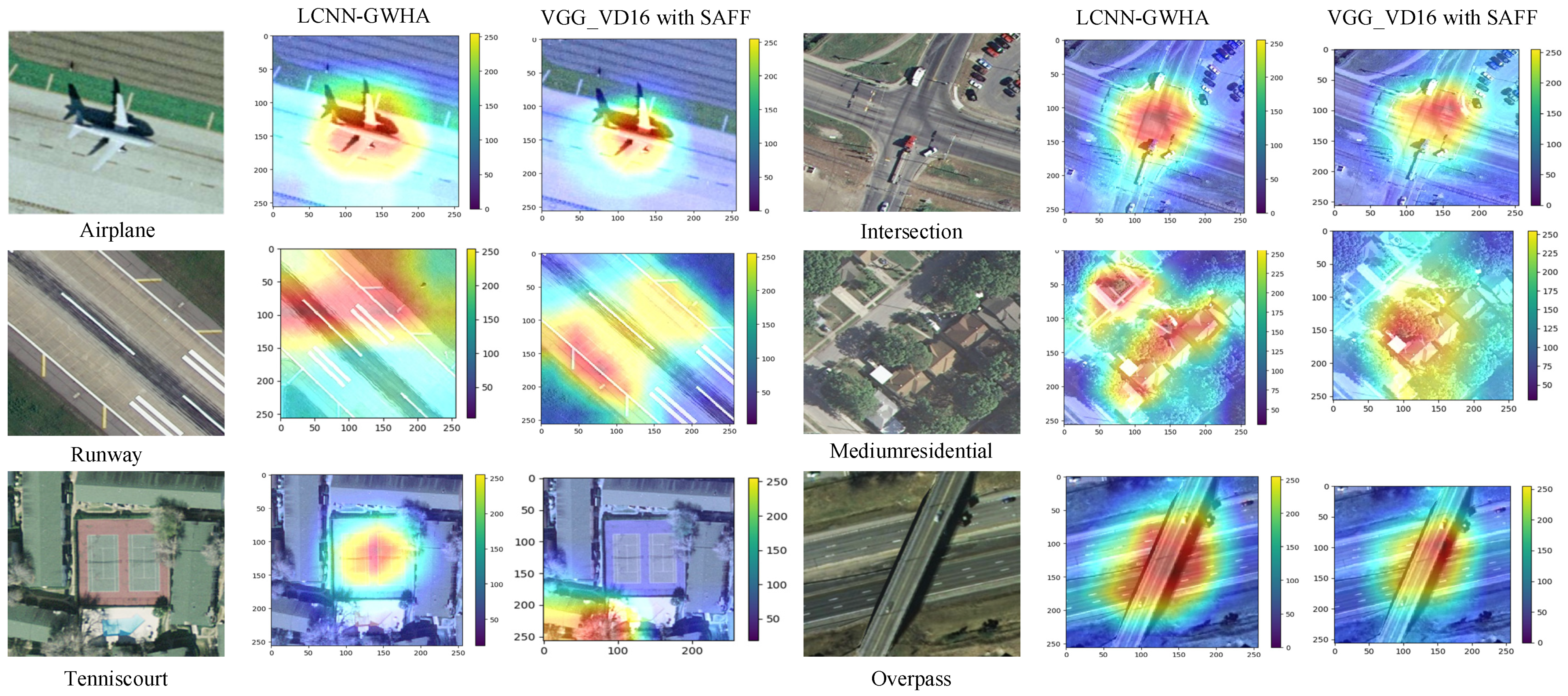
| VGG_VD16 with SAFF [54] | 97.02 ± 0.78 | 15 M |
| Proposed Method | 99.76 ± 0.25 | 0.3 M |
| Network Model | OA (20/80) (%) | OA (50/50) (%) | Number of Parameters |
|---|---|---|---|
| VGG16+CapsNet [39] | 91.63 ± 0.19 | 94.74 ± 0.17 | 130 M |
| VGG_VD16 with SAFF [54] | 90.25 ± 0.29 | 93.83 ± 0.28 | 15 M |
| Discriminative CNN [44] | 90.82 ± 0.16 | 96.89 ± 0.10 | 130 M |
| Fine-tuning [30] | 86.59 ± 0.29 | 89.64 ± 0.36 | 130 M |
| Skip-Connected CNN [43] | 91.10 ± 0.15 | 93.30 ± 0.13 | 6 M |
| LCNN-BFF [38] | 91.66 ± 0.48 | 94.64 ± 0.16 | 6.2 M |
| Gated Bidirectional [41] | 90.16 ± 0.24 | 93.72 ± 0.34 | 18 M |
| Gated Bidirectional+global feature [41] | 92.20 ± 0.23 | 95.48 ± 0.12 | 138 M |
| TSDFF [36] | - | 91.8 | - |
| AlexNet with MSCP [40] | 88.99 ± 0.38 | 92.36 ± 0.21 | - |
| VGG16 with MSCP [40] | 91.52 ± 0.21 | 94.42 ± 0.17 | - |
| ResNet50 [55] | 92.39 ± 0.15 | 94.69 ± 0.19 | 25.61 M |
| InceptionV3 [55] | 93.27 ± 0.17 | 95.07 ± 0.22 | 45.37 M |
| Proposed Method | 93.85 ± 0.16 | 97.64 ± 0.28 | 0.3 M |
| Network Model | OA (10/90) (%) | OA (20/80) (%) | Number of Parameters |
|---|---|---|---|
| R.D [51] | - | 91.03 | - |
| AlexNet with MSCP [40] | 81.70 ± 0.23 | 85.58 ± 0.16 | - |
| VGG16 with MSCP [40] | 85.33 ± 0.17 | 88.93 ± 0.14 | - |
| VGG_VD16 with SAFF [54] | 84.38 ± 0.19 | 87.86 ± 0.14 | 15 M |
| Fine-tuning [30] | 87.15 ± 0.45 | 90.36 ± 0.18 | 130 M |
| Skip-Connected CNN [43] | 84.33 ± 0.19 | 87.30 ± 0.23 | 6 M |
| LCNN-BFF [38] | 86.53 ± 0.15 | 91.73 ± 0.17 | 6.2 M |
| VGG16+CapsNet [39] | 85.05 ± 0.13 | 89.18 ± 0.14 | 130 M |
| Discriminative with AlexNet [44] | 85.56 ± 0.20 | 87.24 ± 0.12 | 130 M |
| Discriminative with VGG16 [44] | 89.22 ± 0.50 | 91.89 ± 0.22 | 130 M |
| ResNet50 [55] | 86.23 ± 0.41 | 88.93 ± 0.12 | 25.61 M |
| InceptionV3 [55] | 85.46 ± 0.33 | 87.75 ± 0.43 | 45.37 M |
| Contourlet CNN [33] | 85.93 ± 0.51 | 89.57 ± 0.45 | 12.6 M |
| LiG with RBF kernel [56] | 90.23 ± 0.13 | 93.25 ± 0.12 | 2.07 M |
| Proposed Method | 92.24 ± 0.12 | 94.26 ± 0.25 | 0.31 M |
Publisher’s Note: MDPI stays neutral with regard to jurisdictional claims in published maps and institutional affiliations. |
© 2021 by the authors. Licensee MDPI, Basel, Switzerland. This article is an open access article distributed under the terms and conditions of the Creative Commons Attribution (CC BY) license (https://creativecommons.org/licenses/by/4.0/).
Share and Cite
Shi, C.; Zhang, X.; Sun, J.; Wang, L. A Lightweight Convolutional Neural Network Based on Group-Wise Hybrid Attention for Remote Sensing Scene Classification. Remote Sens. 2022, 14, 161. https://doi.org/10.3390/rs14010161
Shi C, Zhang X, Sun J, Wang L. A Lightweight Convolutional Neural Network Based on Group-Wise Hybrid Attention for Remote Sensing Scene Classification. Remote Sensing. 2022; 14(1):161. https://doi.org/10.3390/rs14010161
Chicago/Turabian StyleShi, Cuiping, Xinlei Zhang, Jingwei Sun, and Liguo Wang. 2022. "A Lightweight Convolutional Neural Network Based on Group-Wise Hybrid Attention for Remote Sensing Scene Classification" Remote Sensing 14, no. 1: 161. https://doi.org/10.3390/rs14010161
APA StyleShi, C., Zhang, X., Sun, J., & Wang, L. (2022). A Lightweight Convolutional Neural Network Based on Group-Wise Hybrid Attention for Remote Sensing Scene Classification. Remote Sensing, 14(1), 161. https://doi.org/10.3390/rs14010161