
Seasonal and Interhemispheric Effects on the Diurnal Evolution of EIA: Assessed by IGS TEC and IRI-2016 over Peruvian and Indian Sectors

 ,
,  ,
,  and
and 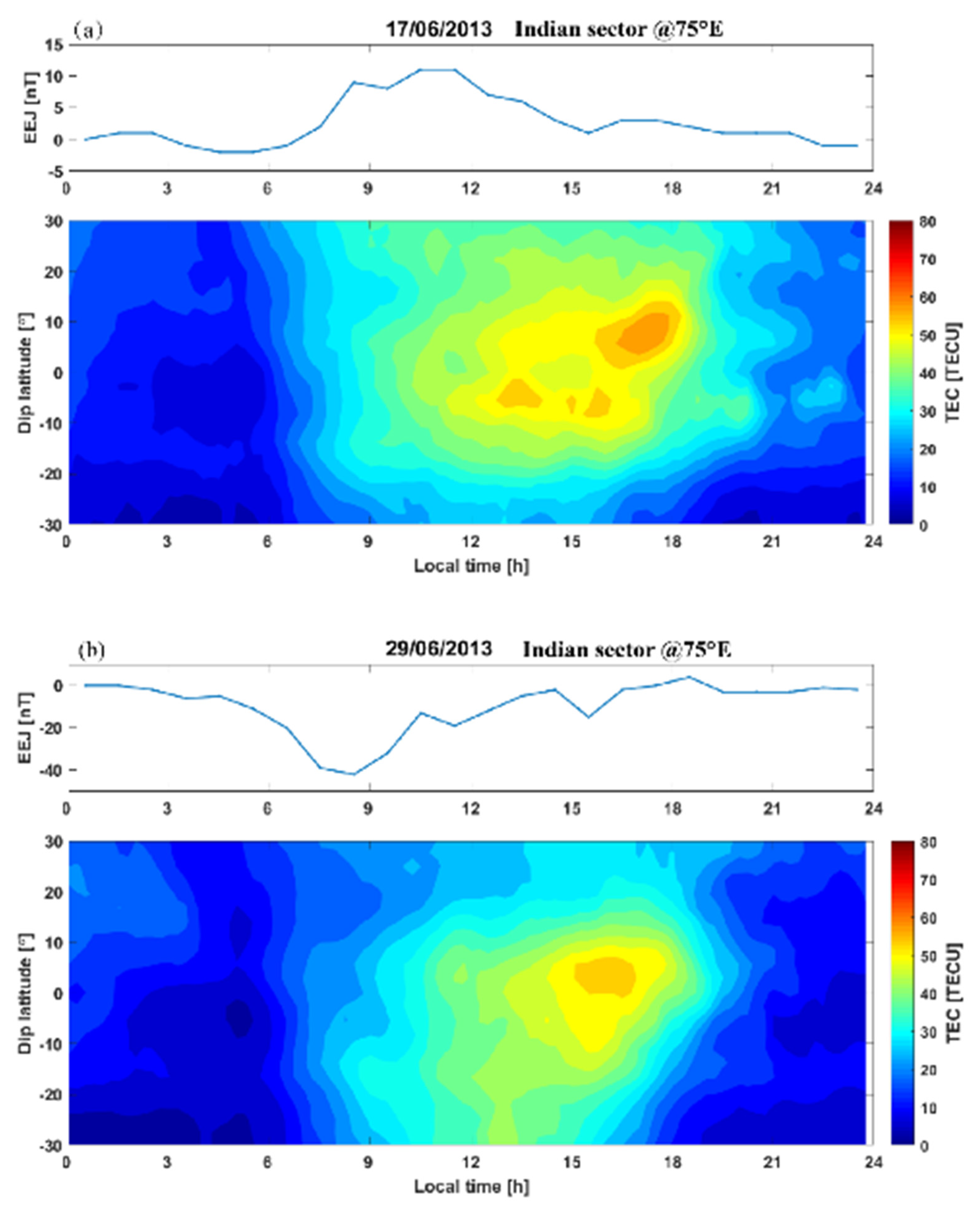
Abstract
:1. Introduction
2. Dataset
2.1. IGS TEC Maps and the IRI-2016 Model
2.2. The EEJ Derived from Ground-Based Magnetometers
2.3. Horizontal Wind Simulated by TIEGCM
3. Methodology and Methods
3.1. Sorting Geomagnetic Quiet Days Using Kp Index
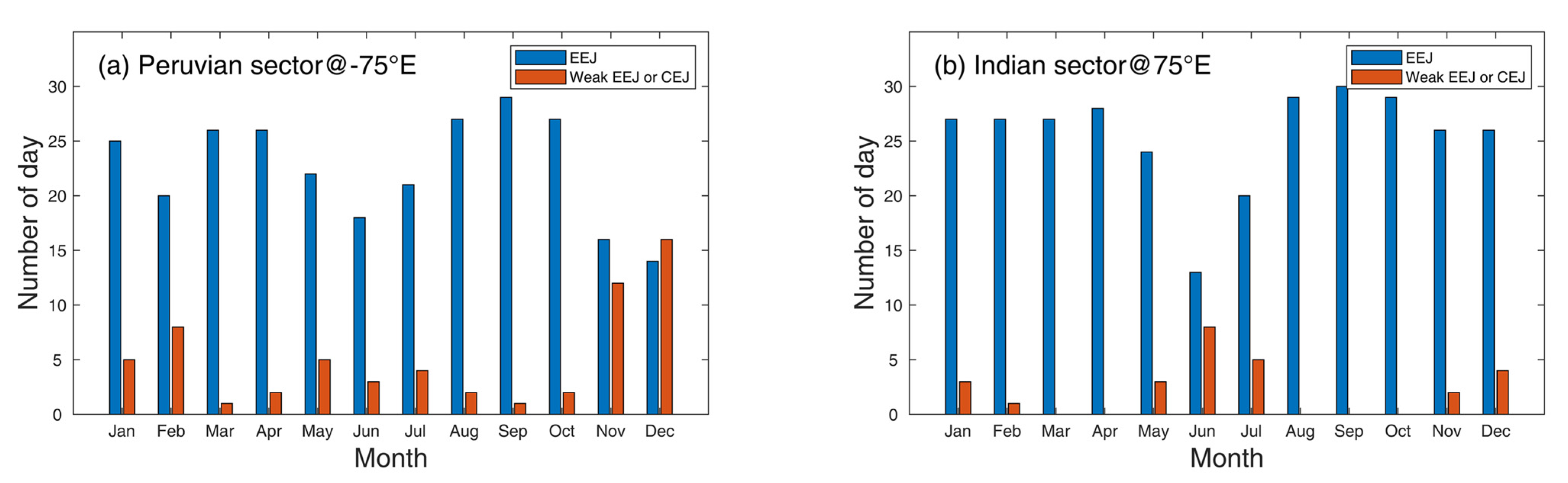
3.2. Sorting Developed EIA Using EEJ as a Proxy
4. Results
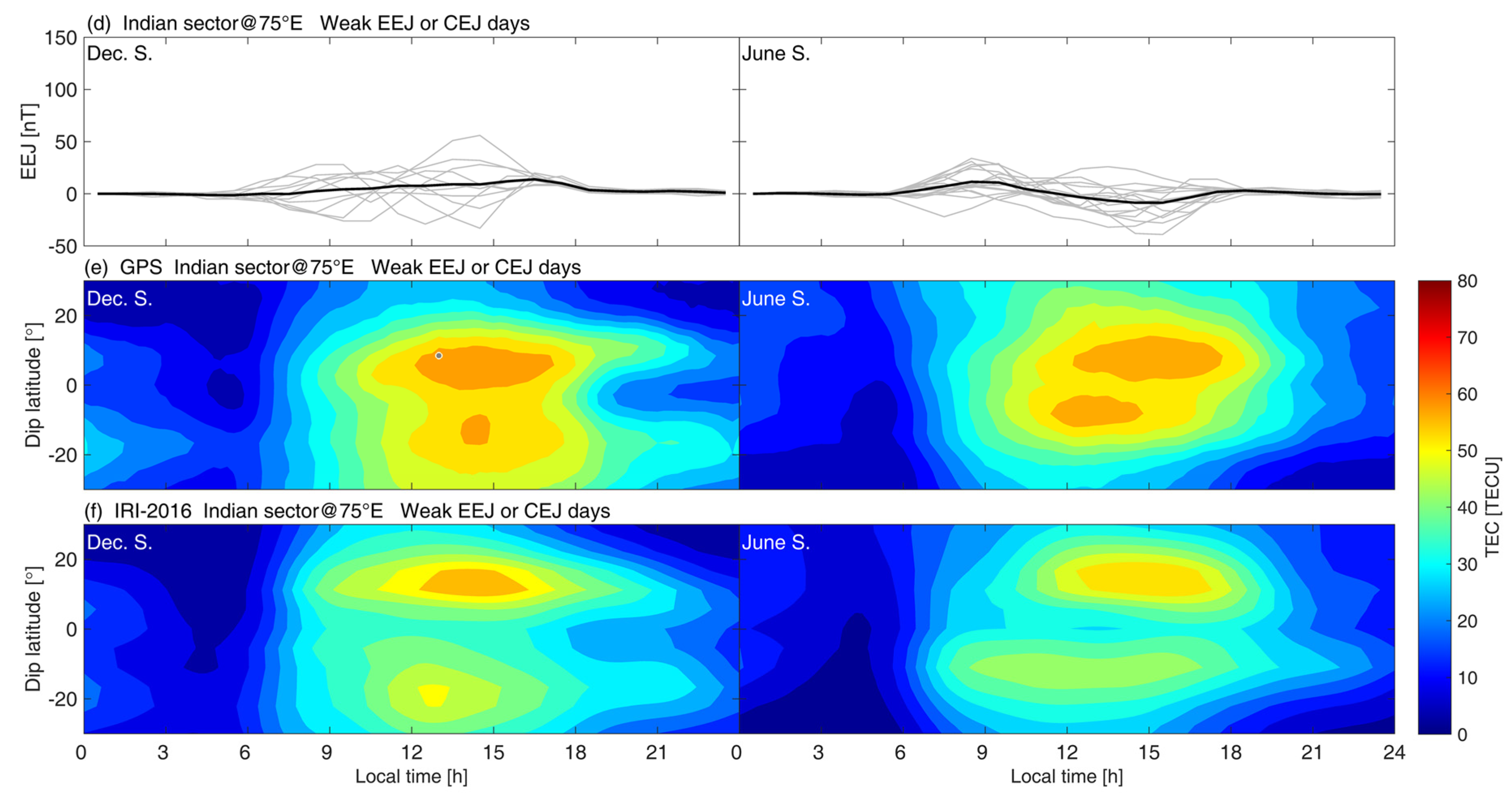
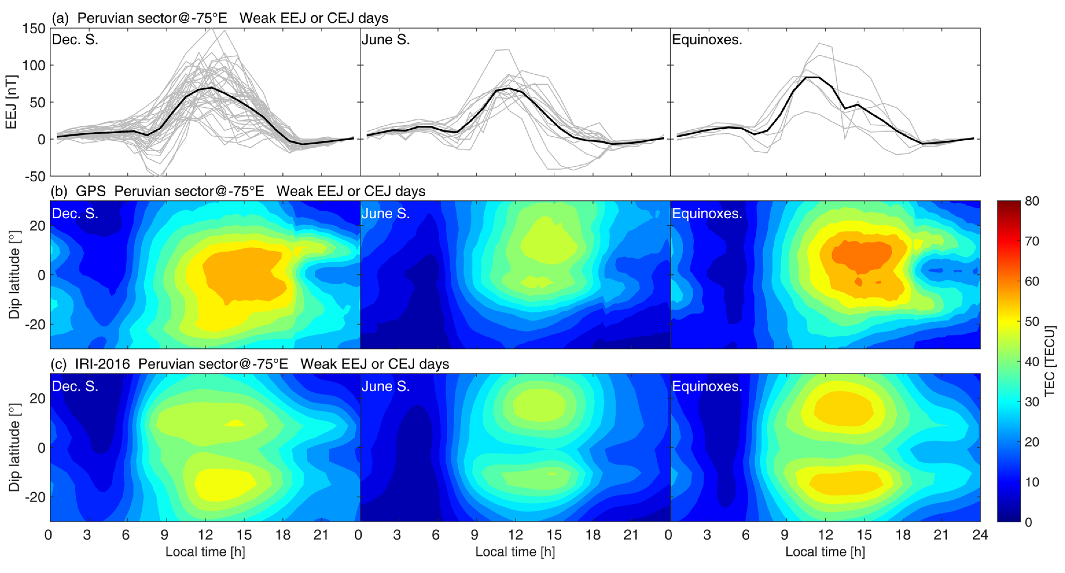
4.1. Overview of EIA during EEJ and Weak EEJ/CEJ Days
4.2. Crest-to-Trough Differences (CTD)
4.3. Time Evolution of EIA: Seasonal and Longitudinal Effects
5. Discussion
6. Conclusions and Future Work Remarks
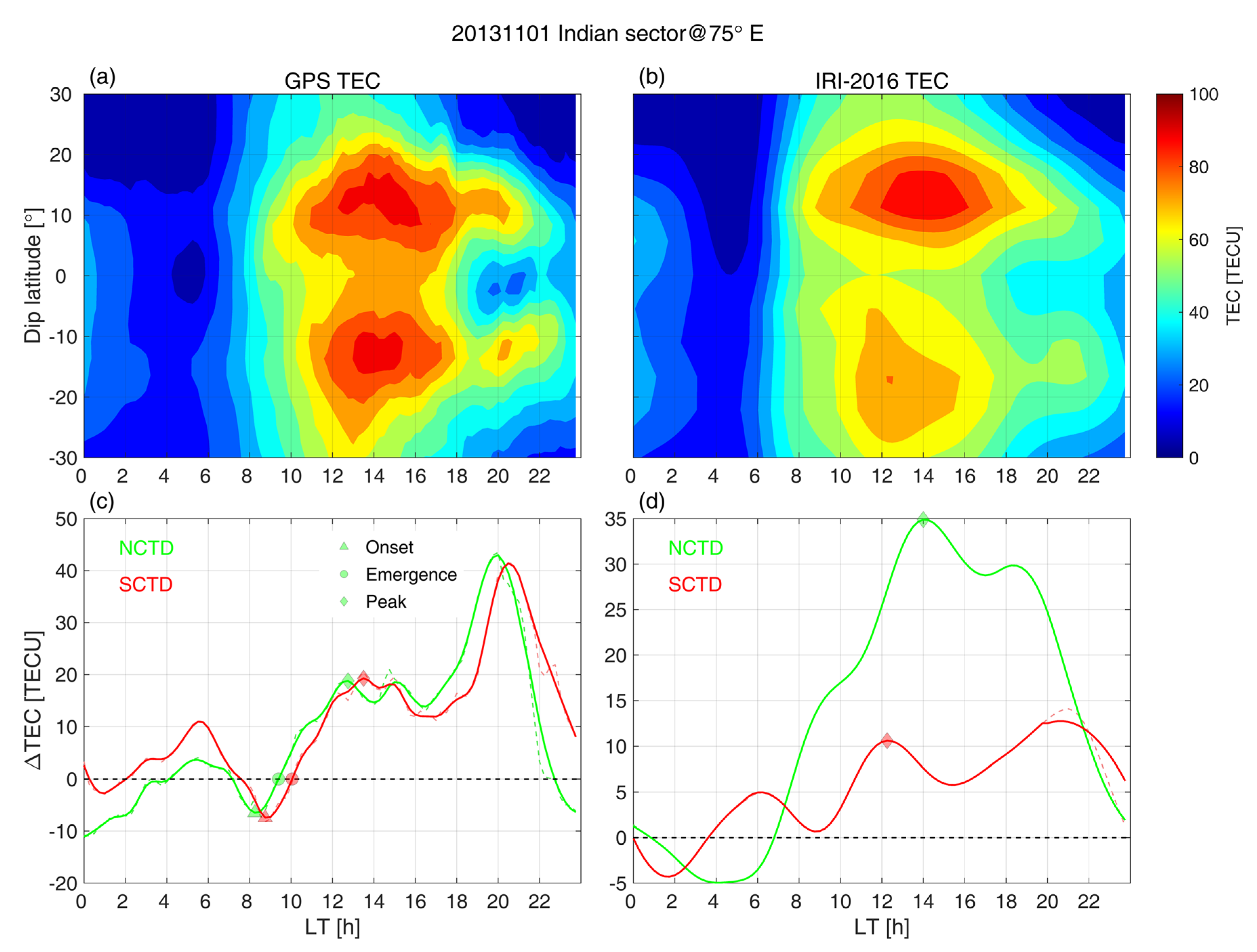
- Three time points can be concluded as: The onset occurs at 0600–1000 LT; the first emergence occurs at 0900–1200 LT; the peak occurs at 1200–1500 LT.
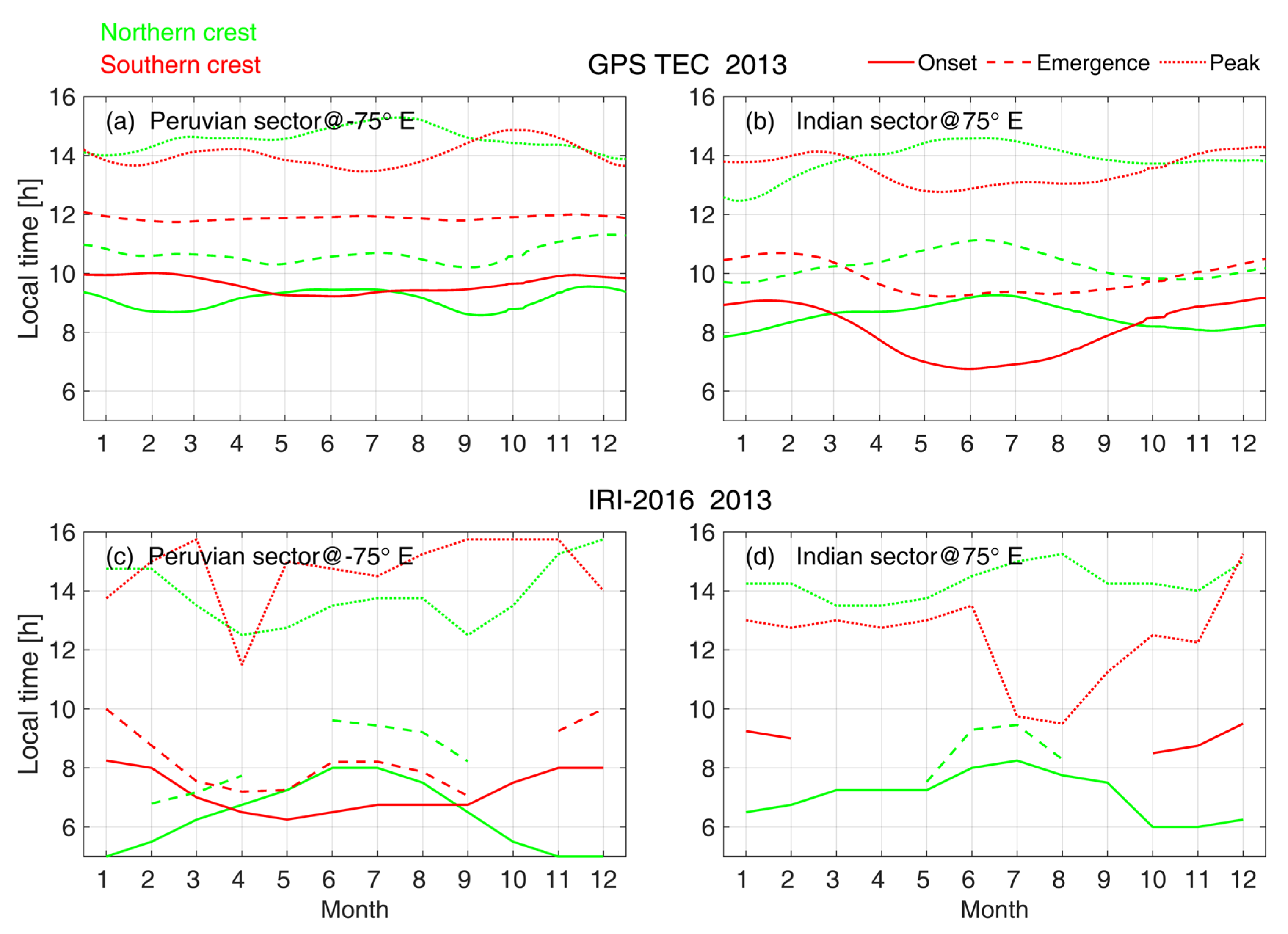
- The onset, first emergence, and peak of EIA show semiannual/annual cycle at the Peruvian/Indian sector. The annual cycle is characterized by a winter priority; that is, the EIA crest during local winter/summer develops earliest/latest. The semiannual is characterized as the northern/southern crest developing earlier during two equinoxes/solstices.
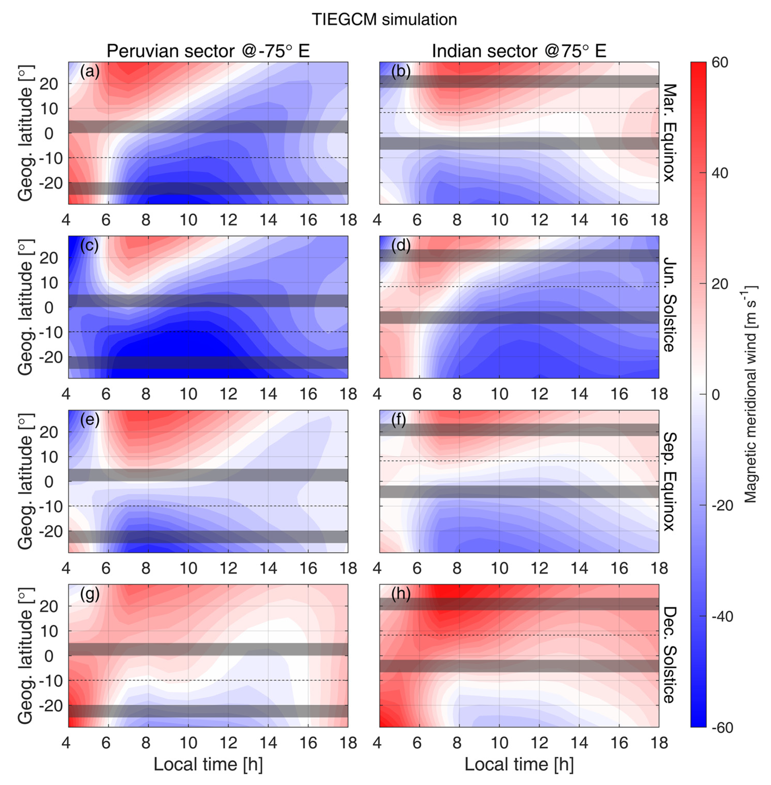
- The winter priority of the annual cycle can be explained by the transequatorial neutral wind that pushes the plasma along the field line to suppress/promote the EIA development in the summer/winter hemisphere. The semi-annual cycle might be associated with the effect of the neutral wind on the modulation of the F region height, which significantly alters the TEC.
- We suggest that the transequatorial wind would not only influence the EIA development via the modulation of ambipolar diffusion but also alter the F region height to further modulate the TEC growth speed. The two effects could be in a completive relationship, which causes complex seasonal variations of the EIA development. More studies are needed to further validate this mechanism.
- The IRI-2016 outputs generally underestimated the TEC value and showed abnormal interhemispheric asymmetry, and sometimes cannot correctly characterize the different stages of the EIA evolution, while the IGS TEC presented a more convincing pattern of the EIA evolution. We suggest that the lack of zonal electric field data that launches the ambipolar diffusion results in IRI’s poor ability to describe the diurnal EIA evolution, and we indicate that the empirical model needs to be further improved. Thus, the I[2]RI-2016 model is not a good candidate to extend this study to longitudes where the GNSS observation is inadequate.
Author Contributions
Funding
Data Availability Statement
Acknowledgments
Conflicts of Interest
References
- Yeh, K.; Franke, S.J.; Andreeva, E.; Kunitsyn, V. An investigation of motions of the equatorial anomaly crest. Geophys. Res. Lett. 2001, 28, 4517–4520. [Google Scholar] [CrossRef]
- Liu, H.; Stolle, C.; Förster, M.; Watanabe, S. Solar activity dependence of the electron density in the equatorial anomaly regions observed by CHAMP. J. Geophys. Res. Space Phys. 2007, 112. [Google Scholar] [CrossRef] [Green Version]
- Xiong, C.; Lühr, H.; Ma, S. The magnitude and inter-hemispheric asymmetry of equatorial ionization anomaly-based on CHAMP and GRACE observations. J. Atmos. Sol.-Terr. Phys. 2013, 105, 160–169. [Google Scholar] [CrossRef]
- Xiong, C.; Zhou, Y.L.; Lühr, H.; Ma, S.Y. Diurnal evolution of the F region electron density local time gradient at low and middle latitudes resolved by the Swarm constellation. J. Geophys. Res. Space Phys. 2016, 121, 9075–9089. [Google Scholar] [CrossRef] [Green Version]
- Chen, Y.; Liu, L.; Le, H.; Wan, W.; Zhang, H. Equatorial ionization anomaly in the low-latitude topside ionosphere: Local time evolution and longitudinal difference. J. Geophys. Res. Space Phys. 2016, 121, 7166–7182. [Google Scholar] [CrossRef]
- Lin, C.; Liu, J.; Fang, T.; Chang, P.; Tsai, H.; Chen, C.; Hsiao, C. Motions of the equatorial ionization anomaly crests imaged by FORMOSAT-3/COSMIC. Geophys. Res. Lett. 2007, 34, L19101. [Google Scholar] [CrossRef]
- Tulasi Ram, S.; Su, S.Y.; Liu, C. FORMOSAT-3/COSMIC observations of seasonal and longitudinal variations of equatorial ionization anomaly and its interhemispheric asymmetry during the solar minimum period. J. Geophys. Res. Space Phys. 2009, 114, A06311. [Google Scholar] [CrossRef]
- Luan, X.; Wang, P.; Dou, X.; Liu, Y.C.M. Interhemispheric asymmetry of the equatorial ionization anomaly in solstices observed by COSMIC during 2007–2012. J. Geophys. Res. Space Phys. 2015, 120, 3059–3073. [Google Scholar] [CrossRef]
- Dang, T.; Luan, X.; Lei, J.; Dou, X.; Wan, W. A numerical study of the interhemispheric asymmetry of the equatorial ionization anomaly in solstice at solar minimum. J. Geophys. Res. Space Phys. 2016, 121, 9099–9110. [Google Scholar] [CrossRef]
- Su, Y.; Bailey, G.; Oyama, K.; Balan, N. A modelling study of the longitudinal variations in the north-south asymmetries of the ionospheric equatorial anomaly. J. Atmos. Sol.-Terr. Phys. 1997, 59, 1299–1310. [Google Scholar] [CrossRef]
- Balan, N.; Rajesh, P.; Sripathi, S.; Tulasiram, S.; Liu, J.; Bailey, G. Modeling and observations of the north–south ionospheric asymmetry at low latitudes at long deep solar minimum. Adv. Space Res. 2013, 52, 375–382. [Google Scholar] [CrossRef]
- Abdu, M. Equatorial ionosphere–thermosphere system: Electrodynamics and irregularities. Adv. Space Res. 2005, 35, 771–787. [Google Scholar] [CrossRef]
- Nanan, B.; Chen, C.; Rajesh, P.; Liu, J.; Bailey, G. Modeling and observations of the low latitude ionosphere-plasmasphere system at long deep solar minimum. J. Geophys. Res. Space Phys. 2012, 117, 8316. [Google Scholar] [CrossRef]
- Liu, J.; Zhang, D.; Mo, X.; Xiong, C.; Hao, Y.; Xiao, Z. Morphological Differences of the Northern Equatorial Ionization Anomaly Between the Eastern Asian and American Sectors. J. Geophys. Res. Space Phys. 2020, 125, e2019JA027506. [Google Scholar] [CrossRef]
- Hernández-Pajares, M.; Juan, J.; Sanz, J.; Orus, R.; Garcia-Rigo, A.; Feltens, J.; Komjathy, A.; Schaer, S.; Krankowski, A. The IGS VTEC maps: A reliable source of ionospheric information since 1998. J. Geod. 2009, 83, 263–275. [Google Scholar] [CrossRef]
- Lühr, H.; Xiong, C. IRI-2007 model overestimates electron density during the 23/24 solar minimum. Geophys. Res. Lett. 2010, 37, L23101. [Google Scholar] [CrossRef] [Green Version]
- Bilitza, D.; Altadill, D.; Reinisch, B.; Galkin, I.; Shubin, V.; Truhlik, V. The international reference ionosphere: Model update 2016. In Proceedings of the EGU General Assembly Conference Abstracts, Vienna, Austria, 17–22 April 2016; p. EPSC2016-9671. [Google Scholar]
- Bilitza, D.; Altadill, D.; Zhang, Y.; Mertens, C.; Truhlik, V.; Richards, P.; McKinnell, L.-A.; Reinisch, B. The International Reference Ionosphere 2012–a model of international collaboration. J. Space Weather. Space Clim. 2014, 4, A07. [Google Scholar] [CrossRef]
- Bilitza, D.; Altadill, D.; Truhlik, V.; Shubin, V.; Galkin, I.; Reinisch, B.; Huang, X. International Reference Ionosphere 2016: From ionospheric climate to real-time weather predictions. Space Weather 2017, 15, 418–429. [Google Scholar] [CrossRef]
- Ren, X.; Chen, J.; Li, X.; Zhang, X.; Freeshah, M. Performance evaluation of real-time global ionospheric maps provided by different IGS analysis centers. GPS Solut. 2019, 23, 113. [Google Scholar] [CrossRef]
- Manoj, C.; Lühr, H.; Maus, S.; Nagarajan, N. Evidence for short spatial correlation lengths of the noontime equatorial electrojet inferred from a comparison of satellite and ground magnetic data. J. Geophys. Res. Space Phys. 2006, 111, A11312. [Google Scholar] [CrossRef]
- Siddiqui, T. Long-Term Investigation of the Lunar Tide in the Equatorial Electrojet during Stratospheric Sudden Warmings. Ph.D. Thesis, Universität Potsdam Potsdam, Potsdam, Germany, 2017. [Google Scholar]
- Heelis, R.; Lowell, J.K.; Spiro, R.W. A model of the high-latitude ionospheric convection pattern. J. Geophys. Res. Space Phys. 1982, 87, 6339–6345. [Google Scholar] [CrossRef]
- Richards, P.; Fennelly, J.; Torr, D. EUVAC: A solar EUV flux model for aeronomic calculations. J. Geophys. Res. Space Phys. 1994, 99, 8981–8992. [Google Scholar] [CrossRef]
- Bartels, J. The standardized Index Ks, and the Planetary index Kp, IATME Bull., 12 (b), 97; IUGG Publ. Office: Paris, France, 1949. [Google Scholar]
- Matzka, J.; Stolle, C.; Yamazaki, Y.; Bronkalla, O.; Morschhauser, A. The Geomagnetic Kp Index and Derived Indices of Geomagnetic Activity. Space Weather 2021, 19, e2020SW002641. [Google Scholar] [CrossRef]
- Stolle, C.; Manoj, C.; Lühr, H.; Maus, S.; Alken, P. Estimating the daytime equatorial ionization anomaly strength from electric field proxies. J. Geophys. Res. Space Phys. 2008, 113, A09310. [Google Scholar] [CrossRef]
- Venkatesh, K.; Fagundes, P.R.; Prasad, D.V.; Denardini, C.M.; De Abreu, A.; De Jesus, R.; Gende, M. Day-to-day variability of equatorial electrojet and its role on the day-to-day characteristics of the equatorial ionization anomaly over the Indian and Brazilian sectors. J. Geophys. Res. Space Phys. 2015, 120, 9117–9131. [Google Scholar] [CrossRef] [Green Version]
- RG, R.; Alex, S.; Patil, A. Seasonal variations of geomagnetic D, H and Z fields at low latitudes. J. Geomagn. Geoelectr. 1994, 46, 115–126. [Google Scholar] [CrossRef]
- Alken, P.; Maus, S. Spatio-temporal characterization of the equatorial electrojet from CHAMP, Ørsted, and SAC-C satellite magnetic measurements. J. Geophys. Res. Space Phys. 2007, 112, A09305. [Google Scholar] [CrossRef] [Green Version]
- Doumouya, V.; Vassal, J.; Cohen, Y.; Fambitakoye, O.; Menvielle, M. Equatorial electrojet at African longitudes: First results from magnetic measurements. Proc. Ann. Geophys. 1998, 16, 658–676. [Google Scholar] [CrossRef]
- Mendillo, M.; Lin, B.; Aarons, J. The application of GPS observations to equatorial aeronomy. Radio Sci. 2000, 35, 885–904. [Google Scholar] [CrossRef]
- Zhao, B.; Wan, W.; Liu, L.; Ren, Z. Characteristics of the ionospheric total electron content of the equatorial ionization anomaly in the Asian-Australian region during 1996–2004. Ann. Geophys. 2009, 27, 3861–3873. [Google Scholar] [CrossRef] [Green Version]
- Qian, L.; Burns, A.G.; Solomon, S.C.; Wang, W. Annual/semiannual variation of the ionosphere. Geophys. Res. Lett. 2013, 40, 1928–1933. [Google Scholar] [CrossRef]
- Rishbeth, H. How the thermospheric circulation affects the ionospheric F2-layer. J. Atmos. Sol.-Terr. Phys. 1998, 60, 1385–1402. [Google Scholar] [CrossRef]
- Zhao, B.; Wan, W.; Liu, L.; Mao, T.; Ren, Z.; Wang, M.; Christensen, A. Features of annual and semiannual variations derived from the global ionospheric maps of total electron content. Ann. Geophys. 2007, 25, 2513–2527. [Google Scholar] [CrossRef] [Green Version]
- Alken, P. A quiet time empirical model of equatorial vertical plasma drift in the Peruvian sector based on 150 km echoes. J. Geophys. Res. Space Phys. 2009, 114, A02308. [Google Scholar] [CrossRef] [Green Version]
- Chaitanya, P.P.; Patra, A. A neural network-based model for daytime vertical E× B drift in the Indian sector. J. Geophys. Res. Space Phys. 2020, 125, e2020JA027832. [Google Scholar] [CrossRef]
- Fejer, B.G. Low latitude electrodynamic plasma drifts: A review. J. Atmos. Terr. Phys. 1991, 53, 677–693. [Google Scholar] [CrossRef]
- Wu, C.-C.; Liou, K.; Shan, S.-J.; Tseng, C.-L. Variation of ionospheric total electron content in Taiwan region of the equatorial anomaly from 1994 to 2003. Adv. Space Res. 2008, 41, 611–616. [Google Scholar] [CrossRef]
- Bello, S.; Abdullah, M.; Hamid, N.A.; Reinisch, B.; Yoshikawa, A.; Fujimoto, A. Response of ionospheric profile parameters to equatorial electrojet over Peruvian station. Earth Space Sci. 2019, 6, 617–628. [Google Scholar] [CrossRef] [Green Version]


Publisher’s Note: MDPI stays neutral with regard to jurisdictional claims in published maps and institutional affiliations. |
© 2021 by the authors. Licensee MDPI, Basel, Switzerland. This article is an open access article distributed under the terms and conditions of the Creative Commons Attribution (CC BY) license (https://creativecommons.org/licenses/by/4.0/).
Share and Cite
Wan, X.; Zhong, J.; Xiong, C.; Wang, H.; Liu, Y.; Li, Q.; Kuai, J.; Cui, J. Seasonal and Interhemispheric Effects on the Diurnal Evolution of EIA: Assessed by IGS TEC and IRI-2016 over Peruvian and Indian Sectors. Remote Sens. 2022, 14, 107. https://doi.org/10.3390/rs14010107
Wan X, Zhong J, Xiong C, Wang H, Liu Y, Li Q, Kuai J, Cui J. Seasonal and Interhemispheric Effects on the Diurnal Evolution of EIA: Assessed by IGS TEC and IRI-2016 over Peruvian and Indian Sectors. Remote Sensing. 2022; 14(1):107. https://doi.org/10.3390/rs14010107
Chicago/Turabian StyleWan, Xin, Jiahao Zhong, Chao Xiong, Hui Wang, Yiwen Liu, Qiaoling Li, Jiawei Kuai, and Jun Cui. 2022. "Seasonal and Interhemispheric Effects on the Diurnal Evolution of EIA: Assessed by IGS TEC and IRI-2016 over Peruvian and Indian Sectors" Remote Sensing 14, no. 1: 107. https://doi.org/10.3390/rs14010107
APA StyleWan, X., Zhong, J., Xiong, C., Wang, H., Liu, Y., Li, Q., Kuai, J., & Cui, J. (2022). Seasonal and Interhemispheric Effects on the Diurnal Evolution of EIA: Assessed by IGS TEC and IRI-2016 over Peruvian and Indian Sectors. Remote Sensing, 14(1), 107. https://doi.org/10.3390/rs14010107