Evaluating Total Electron Content (TEC) Detrending Techniques in Determining Ionospheric Disturbances during Lightning Events in A Low Latitude Region

Abstract

Total Electron Content (TEC) from Global Navigation Satellite Systems (GNSS) is used to ascertain the impact of space weather events on navigation and communication systems. TEC is detrended by several methods to show this impact. Information from the detrended TEC may or may not necessarily represent a geophysical parameter. In this study, two commonly used detrending methods, Savitzky–Golay filter and polynomial fitting, are evaluated during thunderstorm events in Hong Kong. A two-step approach of detection and distinguishing is introduced alongside linear correlation in order to determine the best detrending model. Savitzky–Golay filter on order six and with a time window length of 120 min performed the best in detecting lightning events, and had the highest moderate positive correlation of 0.4. That the best time frame was 120 min suggests that the observed disturbances could be travelling ionospheric disturbance (TID), with lightning as the potential source.

1. Introduction

Total electron content (TEC) obtained from Global Navigation Satellite Systems (GNSS) can be used to ascertain the impact of space weather events on communication and navigation systems. The spatio-temporally wide range of capabilities of GNSS make it useful in studying these impacts. One technique in using GNSS to reveal weather impacts is by detrending the original TEC [1]. That is, a best fit model or method is first fitted or applied to the original TEC, then the difference between the original TEC and the best fit model is computed. The difference obtained can determine amplitude, frequency, and other signal changes in case of a weather event.

Over time, different best fit models have been used. Each best fit method produces different results, which may or may not necessarily detect the impact a weather event makes on the signal or adequately show the occurrence of the event. In using GNSS for space weather event studies, extensive studies have been done on geomagnetic storms [2,3,4], earthquakes [5,6], and typhoons [7,8,9]. The fitting methods have been mostly used in these studies to detect travelling ionosphere disturbance (TID) and other ionosphere irregularities.

Thunderstorms/lightning, a troposphere weather event, have recently garnered interest from the scientific community in the context of harnessing the spatio-temporal capabilities of GNSS to help understand some characteristics of this weather event. Thunderstorm studies in the mid-latitude US plains by Lay, et al. [10] pointed out that ionosphere gravity waves (IGW) damp out before a thunderstorm dies out, contrary to a recent study by Rahmani, et al. [11] in the same study area but at a different time period. Ogunsua, et al. [12] also reported on the ionosphere’s response to thunderstorms in the West African and Congo sector of the equatorial region, stating that thunderstorm impact on the ionosphere at nighttime is negligible compared to the daytime. Mahmud M [13], who also studied thunderstorm events over Southern Africa, showed that a strong correlation exists between hourly lightning and ionosphere irregularity event occurrence. Recent studies by Tang, et al. [14] and Liu, et al. [15] showed the characteristics of thunderstorm generated ionosphere gravity waves (IGW) in the Southern China region.

In contributing to the GNSS and thunderstorm related studies, this study assesses two commonly used fitting methods, the Savitzky–Golay and polynomial methods, to detect lightning events as they have been used to detect the presence of other space events. These two methods have been demonstrated in the existing literature to best indicate the incidence of weather events. The study area is Hong Kong, a low latitude region in the southern China coastal region. In the following sections, a description of the detrending methods is briefly discussed. A two-step approach, used to detect and distinguish lightning from non-lightning events using the detrending methods, is introduced, followed by the results. Discussions on the results and derived conclusions are then presented. Aside from the obvious visual changes in amplitude, statistical means were also used to choose the best fitting method.

2. Materials and Methods

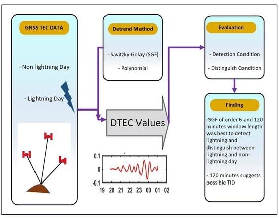
2.1. Detrending Methods

The detrending or best fitting methods adapted in this study are briefly discussed below.

2.1.1. Savitzky–Golay Filter

This filter is named after Abraham Savitzky and Marcel Golay, who first made it known as a solution to smooth out noise in data from a chemical spectrum analyzer. The filter falls into category of low-pass time domain filters that smooth out high data variability [16] and is used in many applications, such as electrocardiogram denoising [17], vegetation monitoring and GNSS-TEC changes. The filter operates by the convolution process, with least squares fitting of successive subsets in a given time window [18]. The formulae and detailed explanation are found in the original work of Savitzky, et al. [19].

2.1.2. Polynomial Filtering

This kind of filter first approximates the entire data set by repeatedly evaluations at a given order. Given a time series F(t) function measured from series x₁, x₂, x₃, ….x_i, the polynomial P is obtained in Equation (1) as

$$P_n\left(X\right)=q_1\left(X^n\right)+q_2\left(X^{n-1}\right)+\dots .+q_n\left(X\right)+q_{n+1}$$

(1)

where $q_n$ are quantities derived based on P using least squares and n is the order. The residuals, or the difference between F(t) and P(X), are computed to filter out gross effects from F(t), from which some useful information can be obtained. An example using TEC time series can be found in Rahmani, et al. [11].

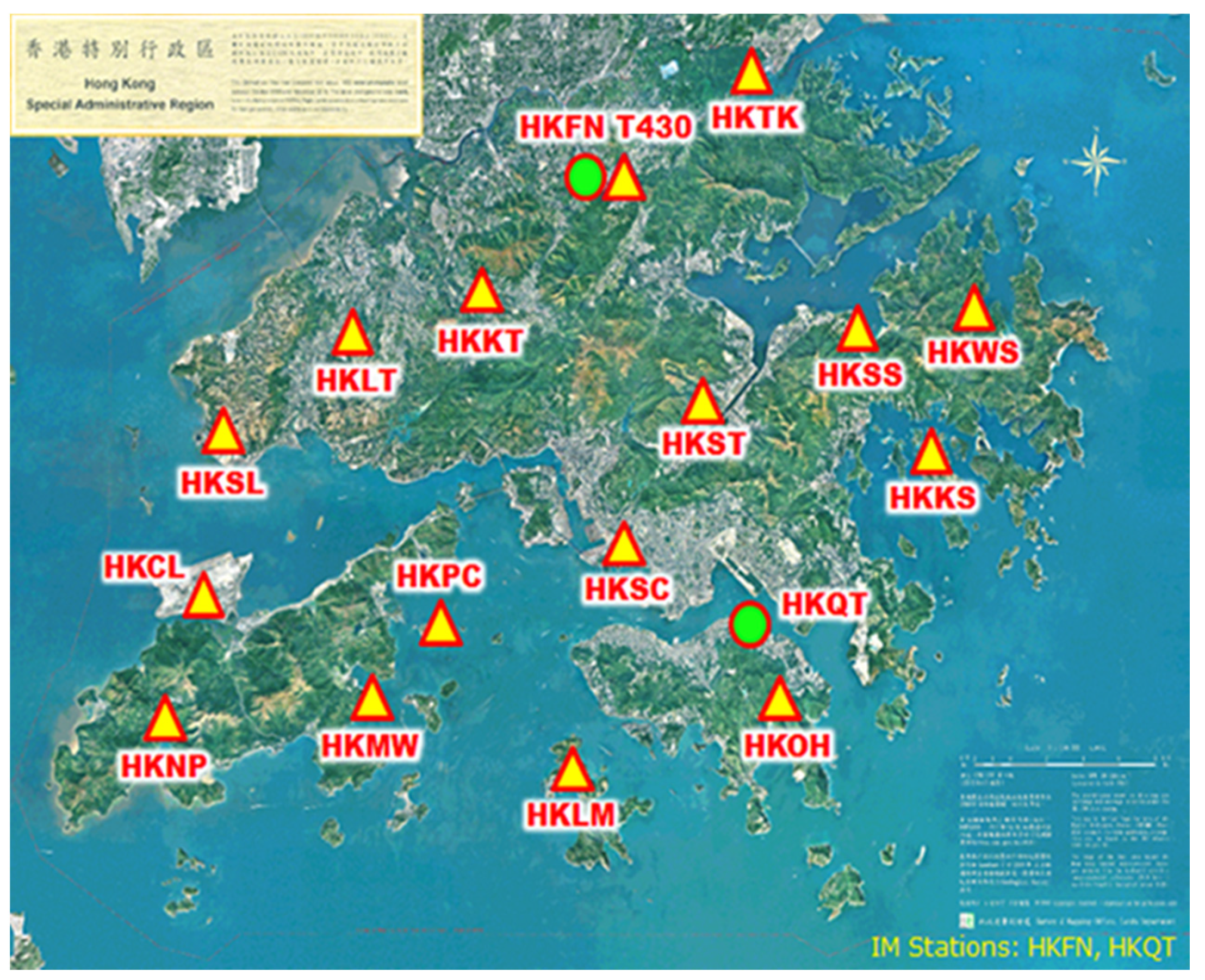
2.2. GNSS Data

The local GNSS network was used to characterize the TEC changes in Hong Kong. The network referred to as Hong Kong Satellite Reference (HK SatRef) covers the entire Hong Kong area. Information on the network is given in the work of Ji, et al. [20]. More details can be obtained from the Hong Kong Survey Department website (https://www.geodetic.gov.hk/en/rinex/downv.aspx (accessed on 14 June 2019)). The American Global Positioning System (GPS) constellation comprising thirty-two satellites was used. Figure 1 shows the study area and GNSS network.

In order to detect ionosphere irregularities caused by lightning, the well-known geometry free linear combination of pseudo- and carrier-phase signals was first used to compute the Slant TEC (STEC) from observations at a sampling interval of 30 s. An elevation cut-off angle of 15° was set to eliminate the multi-path effect [9]. The computed STEC was converted to Vertical TEC (VTEC) by applying a mapping function in Equation (2) below, where R_e is the earth’s radius, θ is the elevation angle at the ionosphere pierce point (IPP) of the signal–receiver path, and h_i is the ionospheric single layer, approximated at 350 km.

$$\mathrm{VTEC}=\sqrt{1-{\left(\frac{R_{e}cos\theta }{R_e+h_i}\right)}^2 }*\mathrm{STEC}$$

(2)

VTEC was then detrended using the two detrending methods stated above to get detrended TEC (DTEC), using Equation (3):

$${\mathrm{DTEC}}_{model}={\mathrm{VTEC}}_{org}-{\mathrm{VTEC}}_{model}$$

(3)

where ${\mathrm{VTEC}}_{org}$ is the original VTEC, ${\mathrm{VTEC}}_{model}$ is the VTEC obtained from the fitting model and ${\mathrm{DTEC}}_{model}$ is the detrended TEC derived according to Equation (3). The unit of VTEC and DTEC is Total Electron Content Units (TECU; 1 TECU = 10¹⁶ e/m² ). Orders of 3 and 6 and time window lengths 30, 60, 90 and 120 min [13,21,22] were selected for Savitzky–Golay, and orders of 3, 5 [23,24], 6, [1,12,25], and 10 [11] were used for polynomial fitting. The selected parameters for detrending are summarized below in

Table 1. Detrending methods and their selected parameters.

Savitzky–Golay
Order	Window (min)
3	30	60	90	120
6	30	60	90	120
Polynomial
Order	3	5	6	10

.

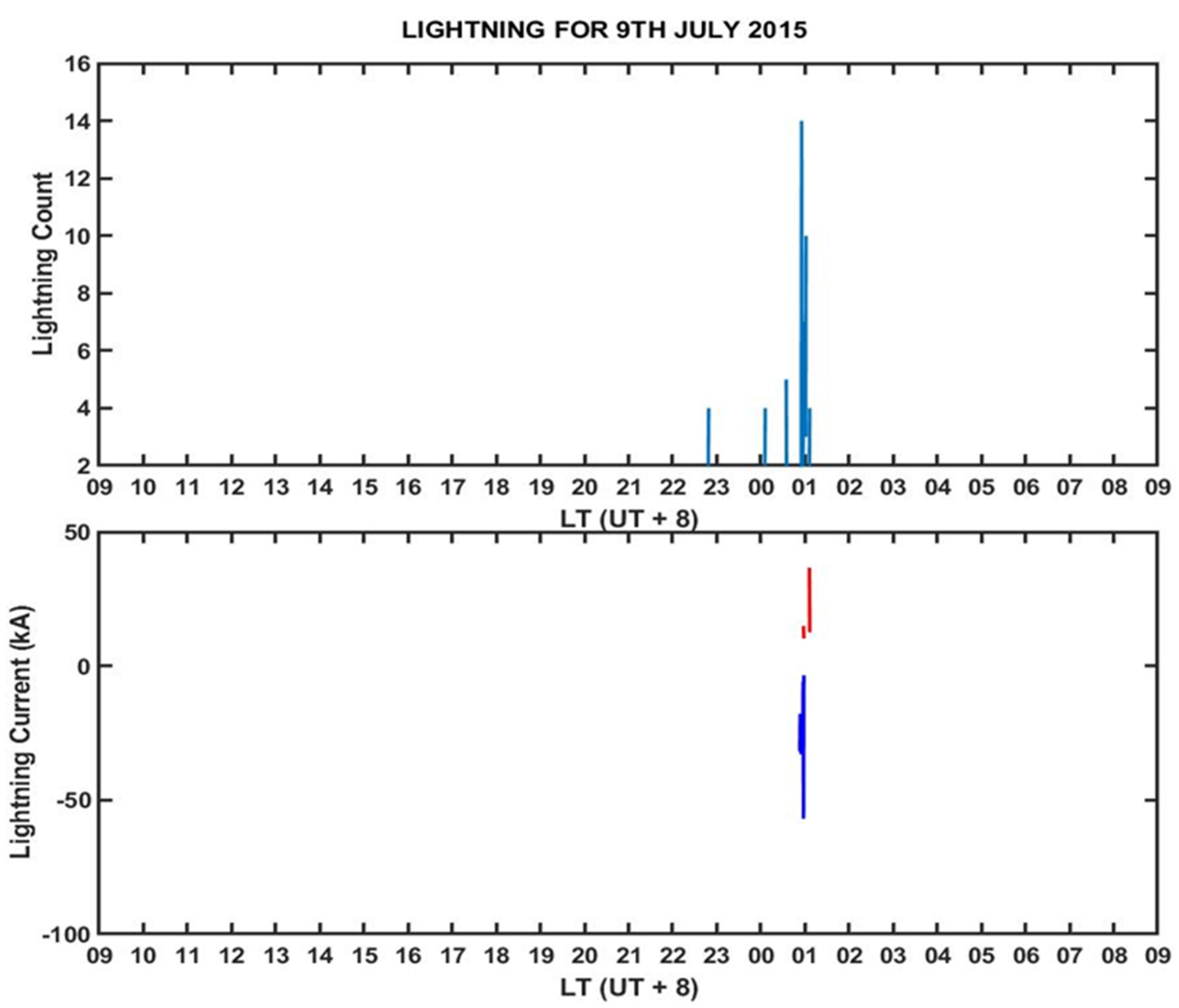
2.3. Thunderstorm/Lightning Data

At very low frequency and low frequency (VLF/LF), lightning discharges produce electric current in the lower D layer of the ionosphere [26]. Lightning data were obtained from a local VLF/LF network in the low-latitude region of Southern China. Total current generated is strongly correlated with lightning activity [27]; a day with a lightning count greater than 10,000 was deemed as a “lightning day”.

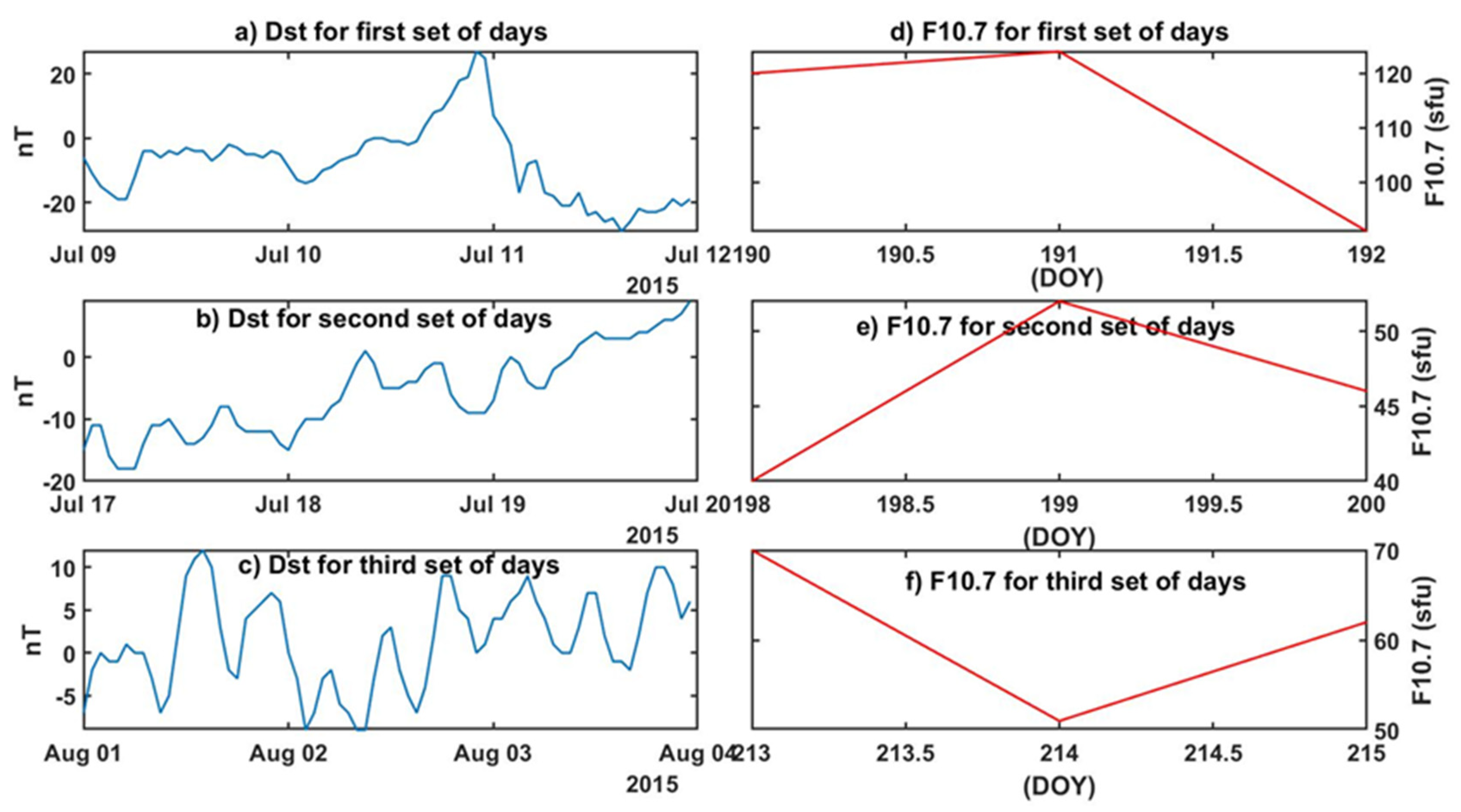
2.4. Selection Criteria

A total of nine days in the months of July and August 2015 were used in this study. The days were grouped into three sets of three. The first (9th to 11th July) and third (1st to 3rd August) sets comprise three continuous non-lightning days before and after the second (17th to 19th July) set of lightning days respectively. The lightning counts for the days are as follows: 319, 1277 and 91 for 9th to 11th July; 200,435, 75,078, and 33,709 for 17th to 19th July; and 6875, 1775 and 1589 for 1st to 3rd August. All days were void of geomagnetic storm or solar condition events. The disturbance storm time (Dst) and solar condition index (F10.7 index) were less than −30 nT [28] and 150 [8], respectively. Figure 2 shows the Dst and F10.7 indices for the set of days.

In determining which detrending method was most suitable for detecting and distinguishing lightning days from non-lightning days, the detection and distinguishing conditions (2DC) approach was used. For the detection condition, because electrical discharge from lightning takes about three hours to travel to higher ionosphere heights, the changes in DTEC amplitude, mostly an increment, may be observed after 3 h of lightning occurrence and last 1–2 h. Being able to show this change using the DTEC method indicates that the DTEC method can detect lightning activity. For the distinguishing condition, anomalous behaviour of DTEC amplitude was checked on non-lightning days against that of lightning days. A non-lightning event day is expected to have one absolute maxima constant as the DTEC amplitude or value throughout, as there is no or little lightning or other space weather events to cause such changes. This constant value is then set as the threshold with which to assess lightning days. As indicated under the detection condition, lightning is expected to cause changes to DTEC amplitude or value. The absolute maximum value of lightning days is compared to the threshold from a non-lightning day. When the increased value is greater than the threshold, a lightning day has either been distinguished from non-lightning days or not. A DTEC method achieving this is said to have both detected lightning activity and distinguished lightning days from non-lightning. Furthermore, 2DC is explained using the following example. Day 1 is a non-lightning day, Day 2 is a lightning day, and the detrending method is DM. First, DM is used to detrend TEC on Day 1. The DTEC on Day 1 was mostly between ± 0.5TECu. Next, TEC on Day 2 is detrended. DTEC on Day 2 was initially ±0.1TECu but at the time of lightning increased to ±0.5TECu. At this point, DM has met the detection condition, and hence is able to detect lightning, but not the distinguish condition, as the DTEC maxima for both days are the same. If Day 2 DTEC at time of lightning increased to, for instance, ±1TECu, DM would have successfully detected and distinguished Day 1 from Day 2. On the other hand, should Day 2 DTEC remain at ±0.1 throughout the entire period, DM could neither detect nor distinguish lightning events from non-lightning event. Figure 3 shows the flow chart of 2DC.

The evaluation was done on the basis of each satellite–receiver pair rather than an average of TEC over a station, in order to obtain greater detail. Satellites passing from the time of lightning occurrence to about 3 h afterwards were investigated.

3. Results

The results are presented in ascending order of set of days. The days in each set are also presented in chronological order. For brevity, the parameters in Table 1 are shortened as follows: polynomials are prefixed by the letter P, followed by the order. For instance, the polynomial of order 3 is represented as P3. That of Savitzky–Golay is prefixed as sgf, followed by the order and window length. For example, the Savitzky–Golay of order 3 with a window length of 30 min is represented as sgf_3_30. Figures showing the lightning count and current are also presented. With TEC and DTEC, the stations of the HK SatRef are quite close; hence, similar observations are made by most stations at a given time [14]. Only observations from station HKOH meeting the criteria in Section 2.4 are presented. A plot of TEC and DTEC for a given satellite in a day has six rows. The first row comprises the original and fitted TEC of P3, P5, P6 and P10 while the second row comprises their respective DTEC. The third row also comprises the original and fitted TEC of sgf_3_30 to sgf_3_120, with the fourth row comprising their respective DTEC. The fifth and last rows follow the same order as the third and fourth rows for sgf_6 parameters. All of the subsequent figures presented showing TEC and DTEC in this section follow the same format.

3.1. First Set of Days (Quiet Days before Lightning Events)

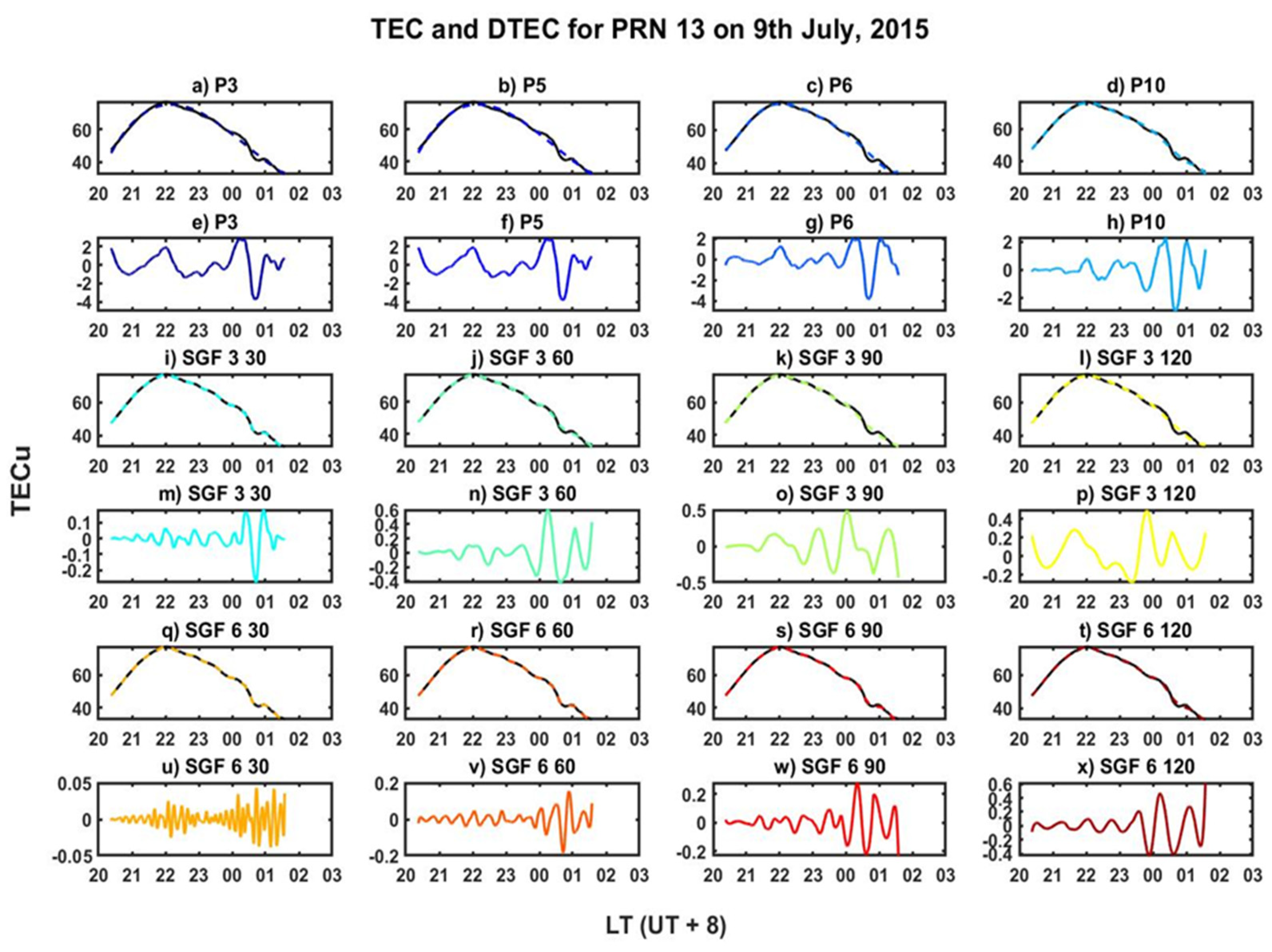
3.1.1. 9th July

This day was the first day of non-lightning days before lightning days. The upper and lower panels of Figure 4 show the lightning count and current, respectively. Few counts are seen from 00–01 local time (LT: UT + 8). Figure 5 and Figure 6 show the TEC-DTEC for satellites of pseudorandom noise code (PRN) 1 and 13. PRN 1 was chosen as it covered the time with no lightning (09–20LT), while PRN 13 was specifically chosen as it covers the time of the few lightning counts.

From panel e of Figure 5, P3 recorded DTEC values between ±3TECu for PRN 1. The amplitudes remained same during the time the satellite was available. For P5, PRN 1 had an amplitude of DTEC of about ±0.5TECu, which remained same throughout the periods. On PRN 13, P5 and P6 had similar characteristics to P3. For P10 the amplitude of DTEC was about ±0.3TECu, which is 0.2 less than that of P5 and P6 on PRN 1. Similar observations to P5 on PRN 13 were made by P10.

Observations on PRN 1 reveal the quiet day phenomena, as no change in amplitude was seen. Increased amplitude on PRN 13 also reveals that P3, P5, P6 and P10 could detect low lightning counts, around 00–01 LT.

sgf_3_30 had an amplitude of DTEC of about ±0.03TECu on PRN 1, shown in panel m of Figure 5, which remained same throughout the day. For sgf_3_60, the amplitude of DTEC was about ±0.1TECu compared to sgf_3_30. sgf_3_90 had an amplitude of DTEC of ±0.5TECu, which was constant for the whole day for PRN 1. sgf_3_120 also had a DTEC amplitude of ±0.2TECu on PRN 1. With PRN 13, sgf_3 parameters saw an increase in amplitude about the same time as lightning. Sgf_3_30 saw an increase to ±0.1TECu, and that of sgf_3_60 to ±0.6TECu. The increases in amplitude for sgf_3_90 and 120 are no different than the amplitude recorded on PRN 1.

The DTEC amplitude of sgf_6_30 was mostly between ±0.01TECu, and remained constant for the whole day on PRN 1. That of sgf_6_60 was between ±0.03TECu compared to sgf_6_30. For sgf_6_90 and 120, the amplitude was about ±0.05TECu compared to sgf_6_30 and sgf_6_60. On PRN 13, sgf_6_30 saw an increase in amplitude of about ±0.05TECu, while sgf_6 30, 90 and 120 saw an increase of about ±0.2TECu during the time of the lightning count.

In all, most parameters had their DTEC amplitude constant throughout the day, and were thus able to represent a quiet day. Sgf parameters had lower amplitudes compared to polynomials.

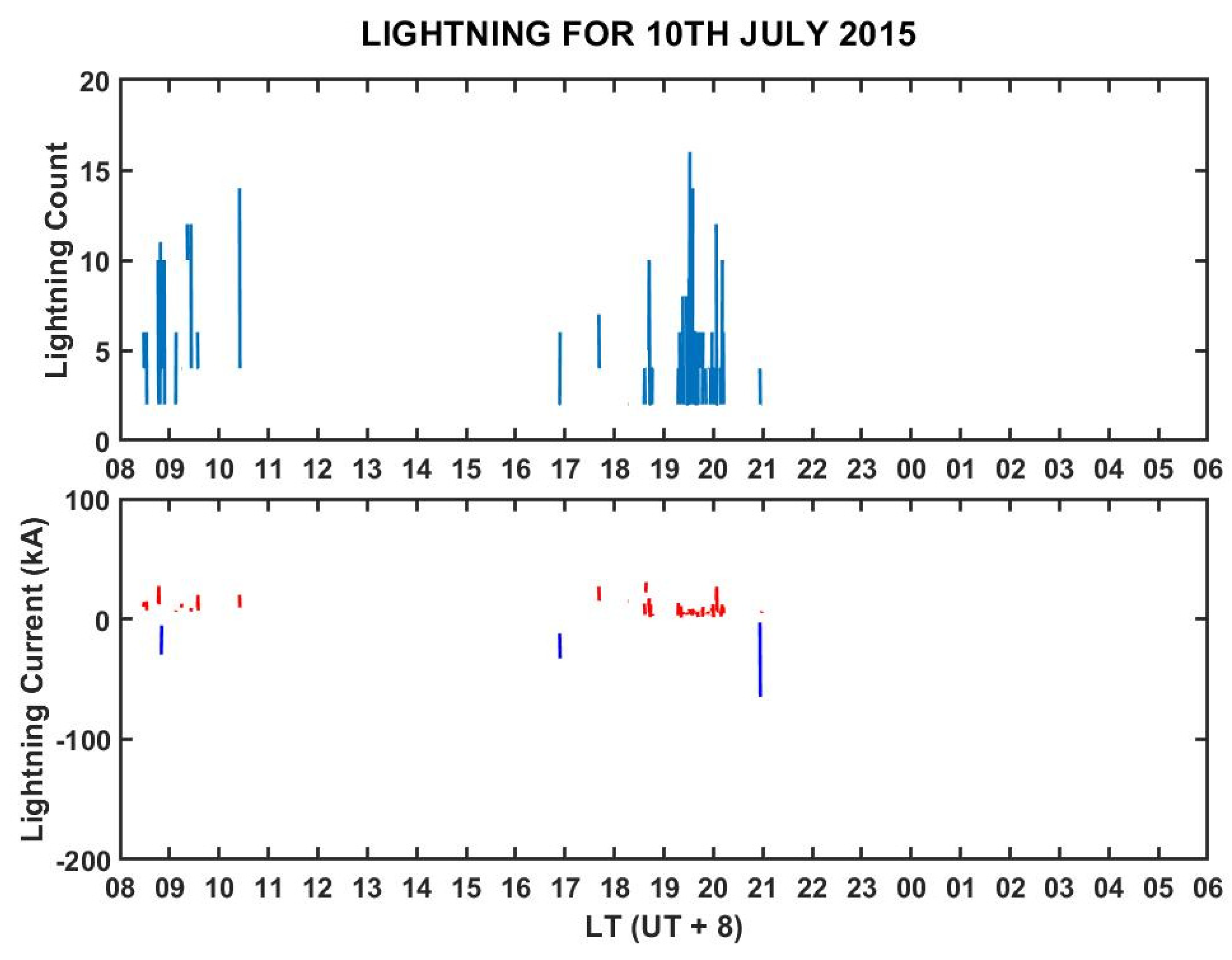
3.1.2. 10th July

This day was the second of the non-lightning days before lightning days. Figure 7 shows the lightning count and current. Few lightning counts were seen at 08–09 and 18–20 LT. Figure 8 shows the TEC-DTECs for PRN 13.

From panels f–h of Figure 8, P5, P6 and P10 all had a constant amplitude of ±0.5TECu. P3 had the highest DTEC value at ±4TECu. The amplitudes remained the same for the whole period

Sgf_3_30 had an amplitude of DTEC of about ±0.05TECu on PRN 13 in Figure 8, and remained constant. Panels n–p in Figure 8 show that sgf_3_60, 90 and 120 had a constant amplitude of ±0.2TECu on PRN 13.

For sgf_6_30, the DTEC amplitude was ±0.02TECu and remained constant for the whole period on PRN 13 (panel u of Figure 8). Sgf_6_60, 90 and 120 recorded DTEC amplitudes of ±0.05TECu throughout the period of PRN 13

Similar to 9th July, most parameters had their DTEC amplitude constant throughout the day, and were thus ably to represent a quiet day. Sgf parameters had lower amplitudes compared to polynomials.

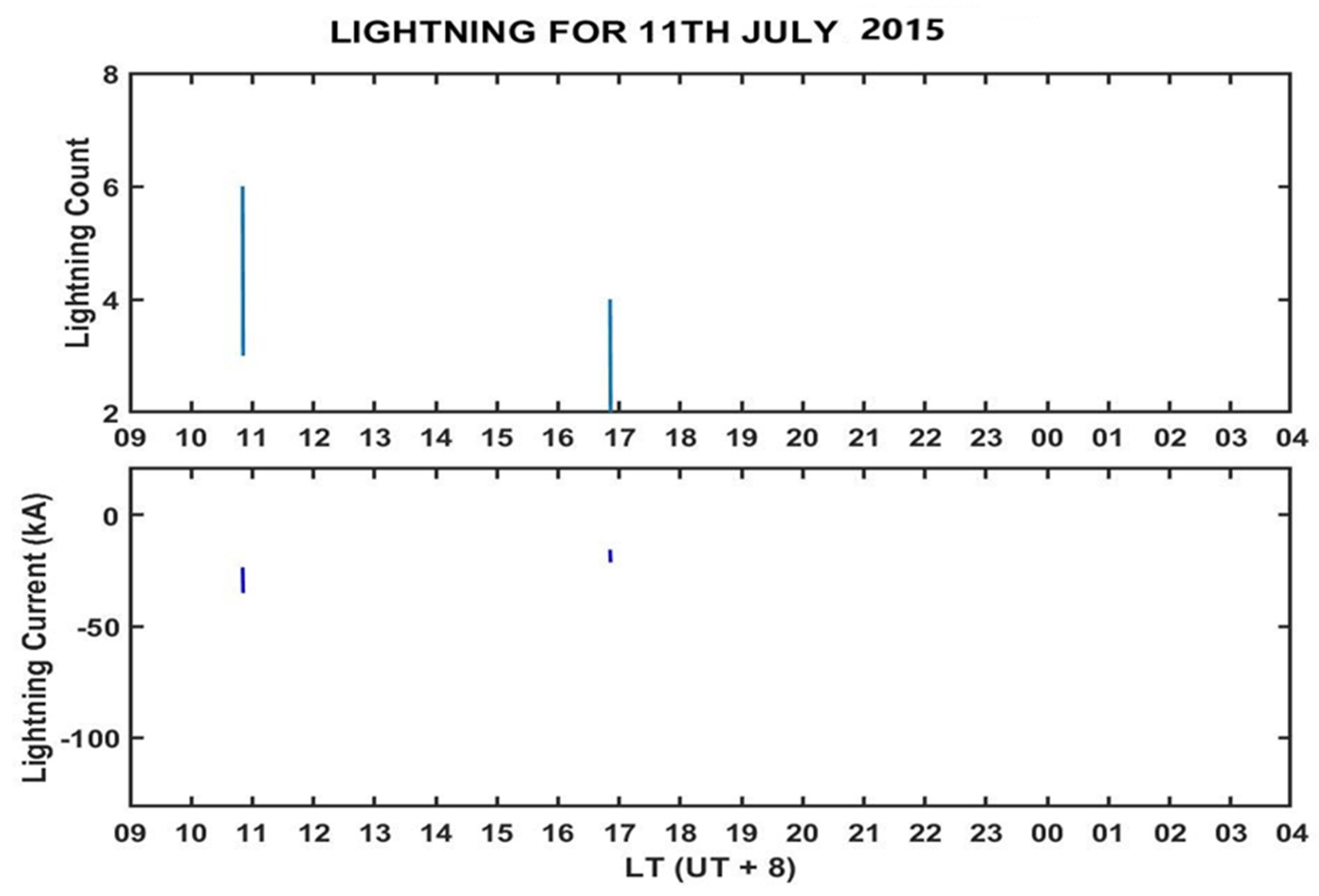
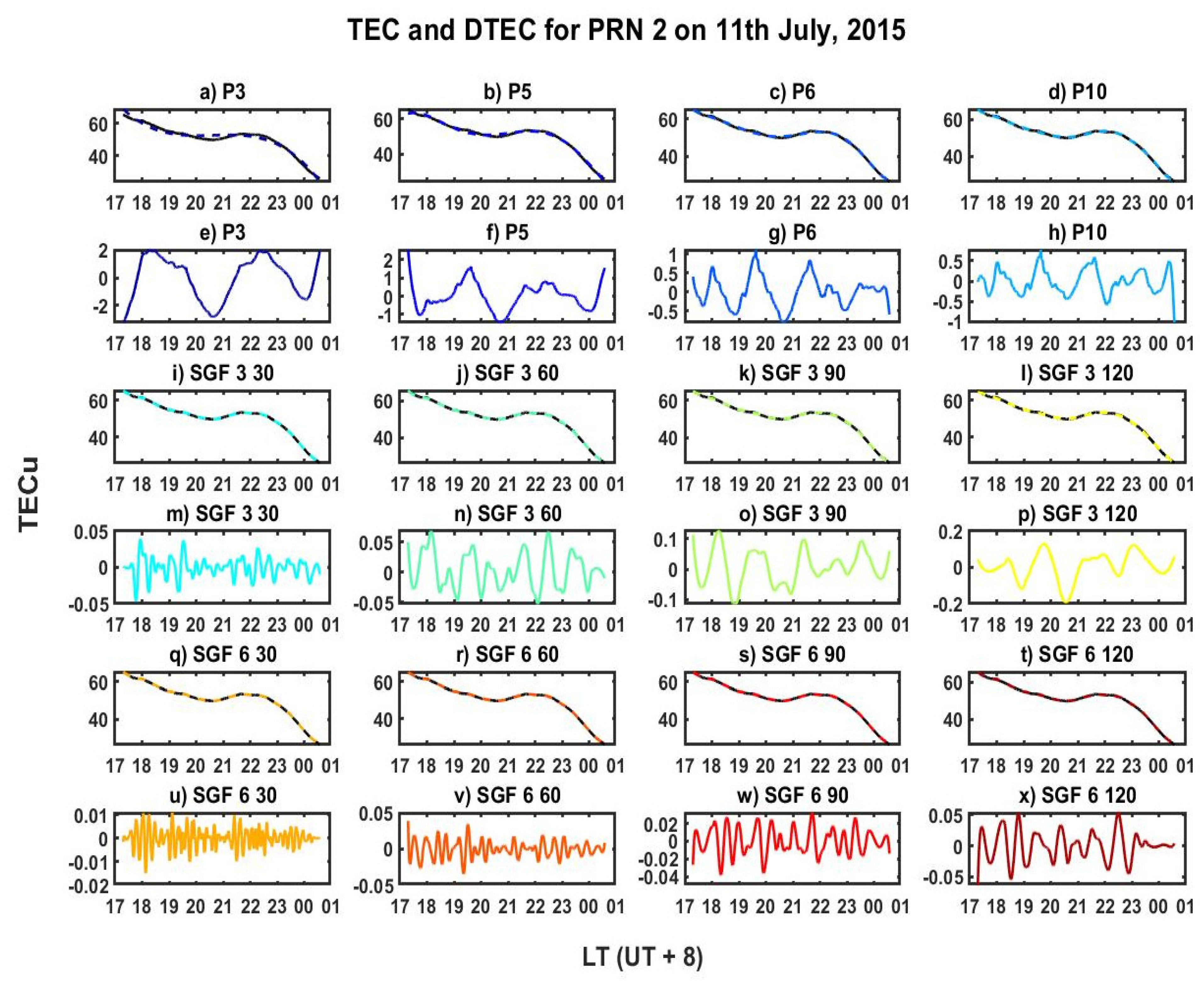
3.1.3. 11th July

This day was the last of the non-lightning days before lightning days. Compared to the previous days in this set of days, 11th July virtually had no lightning count, making it an ideal example of a truly quiet day. Figure 9 shows the lightning count and current. Figure 10 shows the TEC-DTECs for PRN 2. Most satellites had similar observations to PRN 2.

From Figure 10, the polynomial and sgf parameters had constant amplitudes throughout the period of PRN 2. DTECs for all the parameters had similar characteristics to those of 9th and 10th July; this example thus represents a typical quiet day.

3.2. Second Set of Days (Lightning Days)

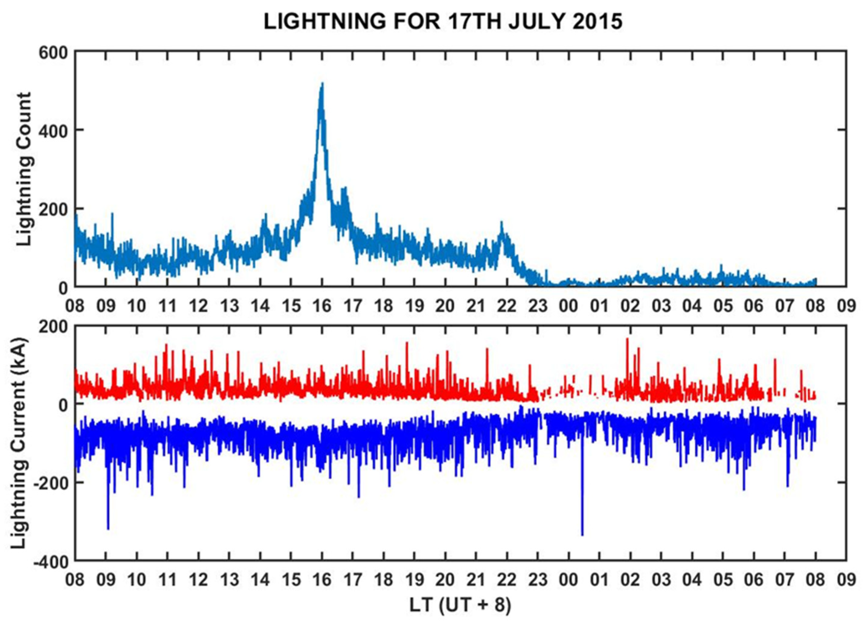
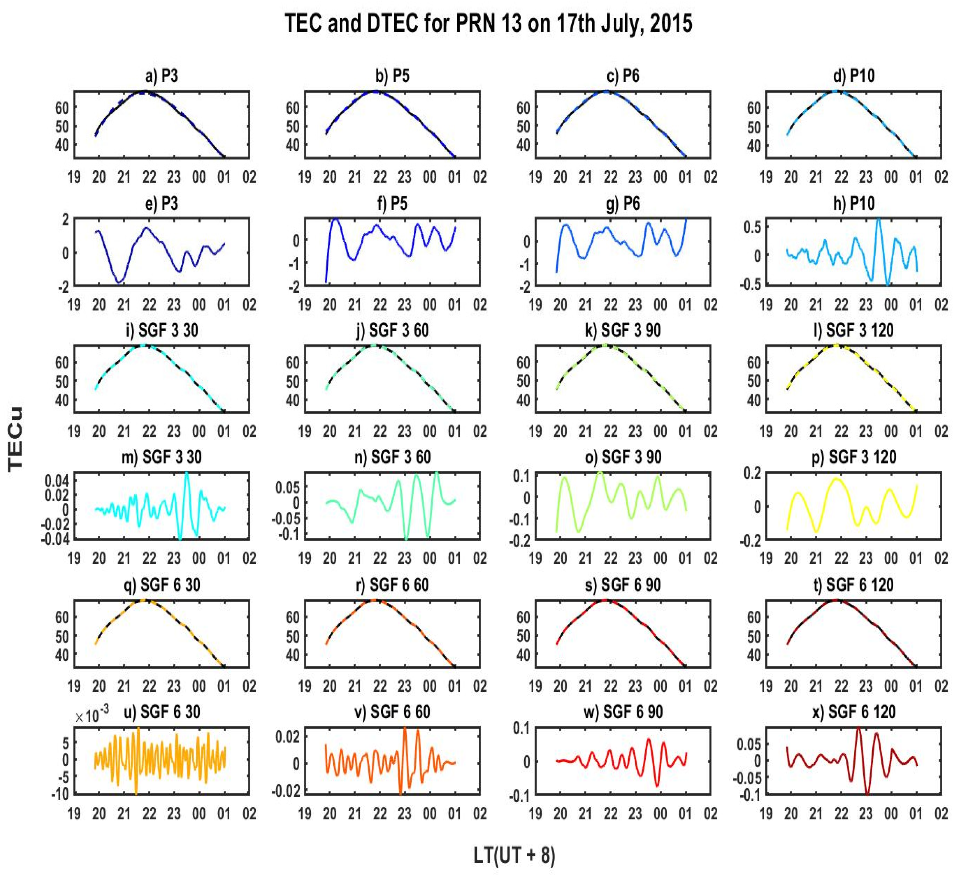
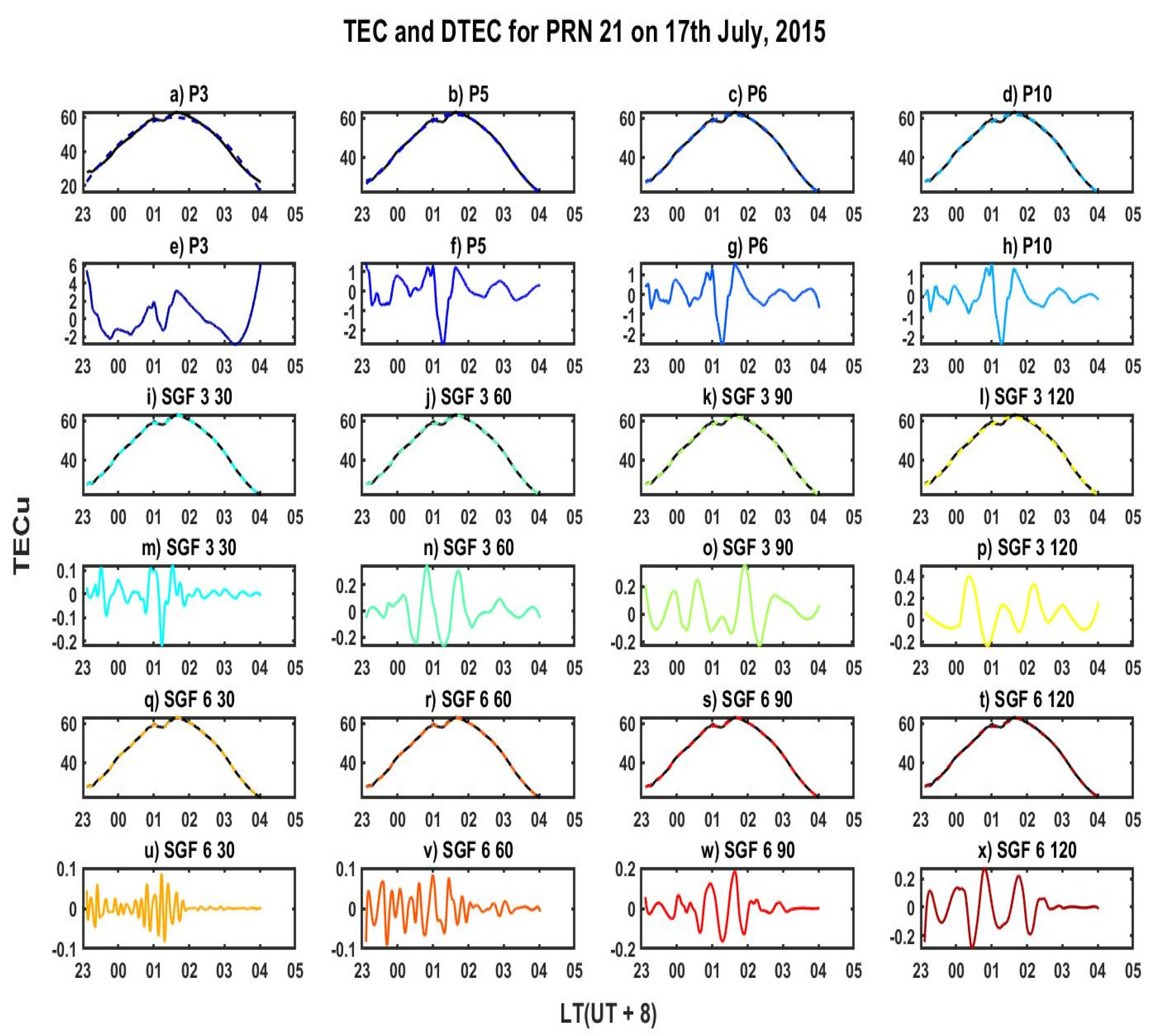
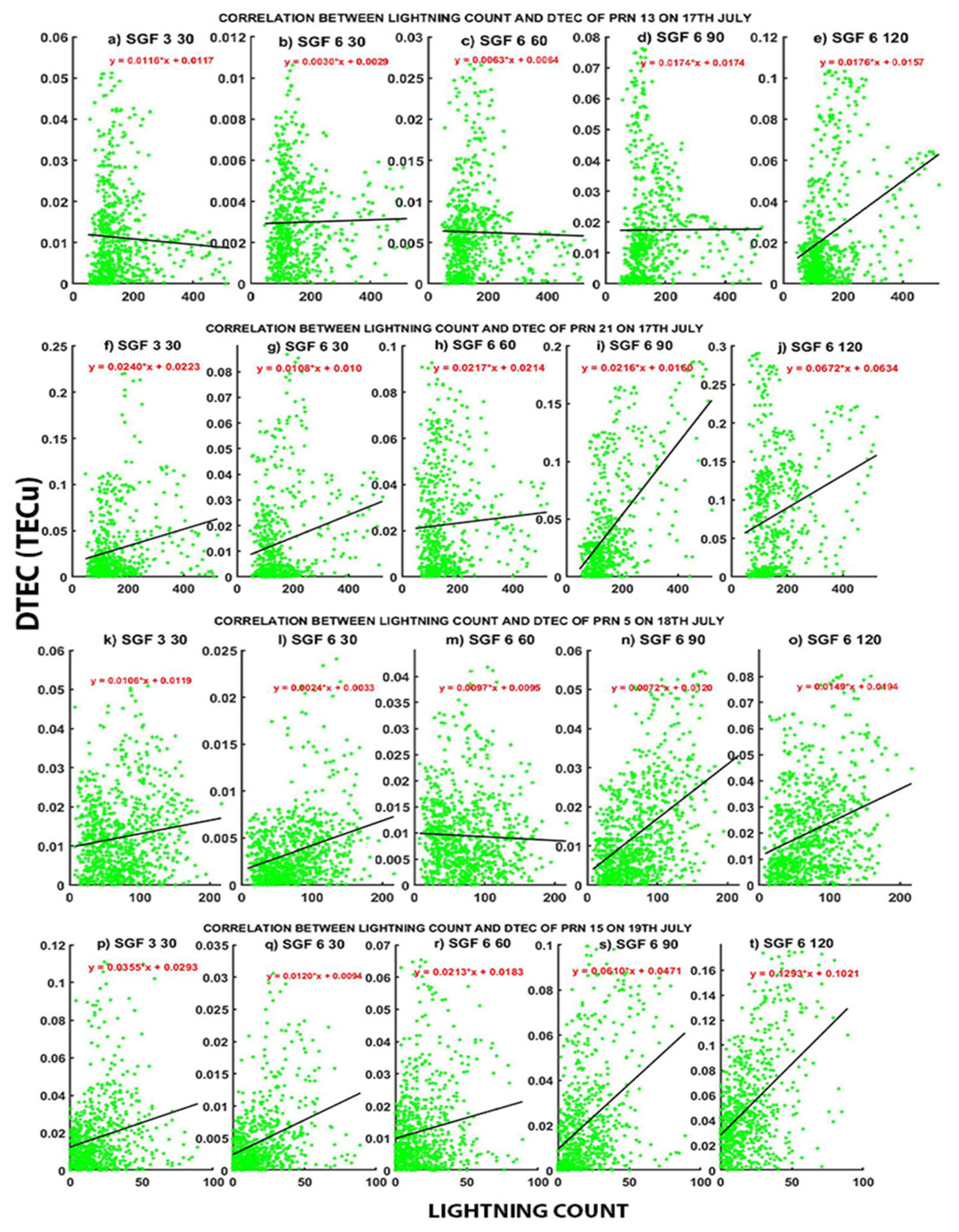
3.2.1. 17th July

This was the first of the lightning days. Lightning happened for the whole day, with a peak count around 15–17 LT. After 22 LT, the lightning activity reduced to a minimum. Lightning activity is shown in Figure 11. TEC and DTEC of PRN 13 and 21 are shown in Figure 12 and Figure 13 to check the changes in DTEC for the first peak expected at 18LT and second peak expected at 01LT, respectively.

Since it takes about three hours for lightning to effect changes in TEC, and the change lasts for about three hours, amplitude changes for the first peak (15–17LT) can be expected to be around 20–23LT, while for the second peak (22LT) they can be expected to show changes of around 00–02LT. In panels e–g in Figure 12, P3, P5 and P6 show the same amplitude values throughout. No increase is seen in the DTEC amplitude values. For P10 in panel f, DTEC amplitude increases to ±0.5TECu at the expected time. P10 was thus able to detect the lightning event on PRN 13. In Figure 13, the DTEC amplitude drops sharply at the expected hour of 01LT from 1 to −2TECu for P5, P6 and P10, signifying a detection. P3 also records a similar observation, though this is not as obvious as P5, P6 and P10.

For the sgf_3 parameters, only sgf_3_30 and 60 could detect the lightning event on PRN 13 in Figure 12. Their amplitudes increased to ±0.04 within the expected time range. Sgf_3_90 and 120, on the other hand, had constant DTEC amplitude. For the second lightning peak at 22LT, all of the sgf_3 parameters could detect it within the expected time range. Their amplitudes increased to between ±0.2–0.4TECu, as seen in panels m to p in Figure 13.

Sgf_6_30 could not detect the first lightning peak but did detect the second. Sgf_6_60, 90 and 120 detected both lightning peaks as increase in amplitude, as seen in panels v to x in Figure 12 and Figure 13.

P5, P6 and P10 could detect lightning events; although the change in amplitude for lightning and non-lightning days were similar, the DTEC amplitude values of sgf parameters indicating the presence of lightning were higher compared to the quiet non-lightning days.

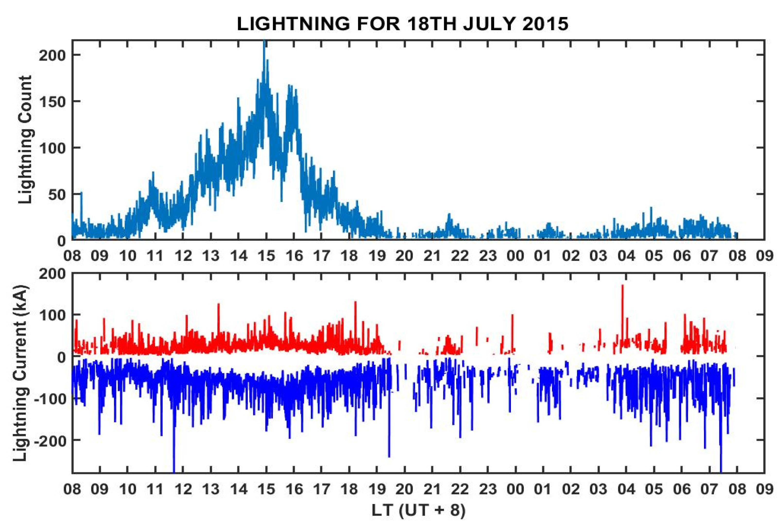
3.2.2. 18th July

This was the second of the lightning days. Lightning happened for the whole day, with peaks around 15LT. At 21LT, a small peak was also seen. Figure 14 shows the lightning event. DTEC-TEC are shown for PRN 5 in Figure 15, as its time of availability covered the expected time of the amplitude changes of the two peaks, 18LT for the peak at 15LT and 23LT for that at 21LT.

With peak counts around 15 and 21LT, changes in DTEC amplitude were expected around 18 and 23LT. P3, P5 and P6 had constant amplitudes of ±3TECu, and hence were not able to detect the lightning event. P10 first saw an increase in amplitude of about ± 0.5TECu, then a reduced amplitude of ±0.2TECu, and finally another increase to ±0.5TECu. These increments all happened at the expected time of amplitude change, indicating that P10 could detect the lightning event. From panels m to p in Figure 15, sgf_3 parameters all saw amplitude changes at the expected time. Sgf_3_30 recorded ±0.06TECu, while sgf_3_60, 90 and 120 all recorded ±0.2TECu at the expected time of DTEC changes. Sgf 6 parameters also showed an increase in DTEC amplitude at the expected time. Sgf_6_30 recorded ±0.03TECu and sgfs 6_60, 90 and 120 all recorded ±0.07TECu.

P10 and all of the sgf parameters therefore detected the lightning activity on this day.

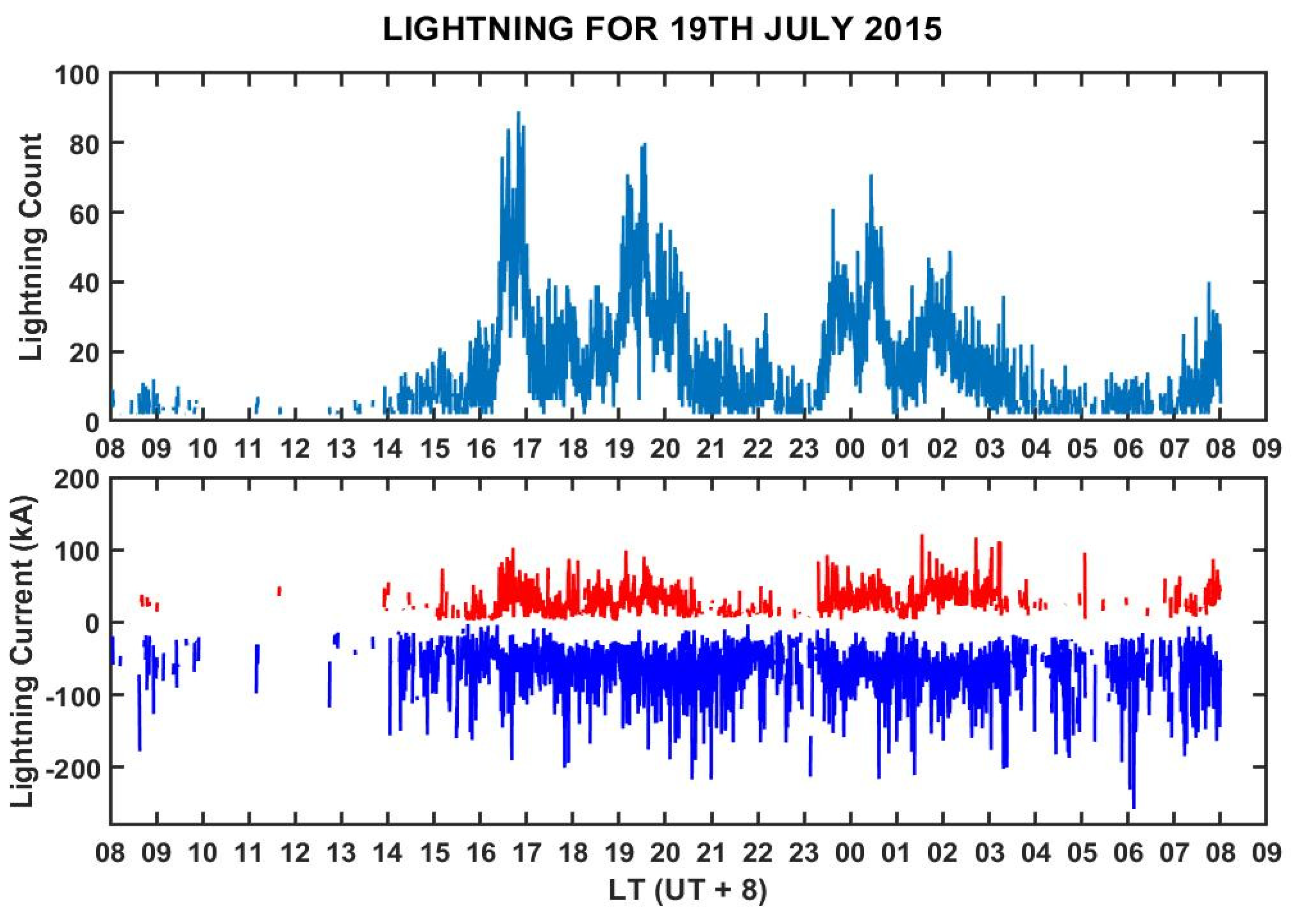
3.2.3. 19th July

This was the last of the lightning days. Lightning happened from 08–09LT and reoccurred from 16–07LT. The peak periods were 16–17, 19–20 and 23–03LT, with DTEC amplitude changes expected at 11, 23 and 02LT, respectively. PRN 15 was available at 20–02LT, covering the expected time changes of the second peak period and hence able to be investigated. Figure 16 and Figure 17 show the lightning activity and DTEC for PRN 15, respectively.

Less useful information could be derived from the DTEC of P3 (panel e of Figure 17 and Figure 18). P5, P6 and P10 made similar observations to PRN 15. An increase in amplitude of ±2TECu was seen around 22–23LT, and the amplitude changes occur at the expected time.

Sgf_3_30, 60, 90 and 120 all saw an increase in DTEC amplitude at the expected time. Similar observations were also made by the sgf_6 parameters. Sgf_3_30 recorded ±0.06TECu, while sgf_3_60, 90 and 120 all recorded ±0.2TECu at the expected time of DTEC changes. Sgf 6 parameters also showed an increase in DTEC amplitude at the expected time. Sgf_6_30 recorded ±0.03TECu, sgf 6_60 and 90 recorded ±0.1TECu, and 6_120 recorded ±0.2TECu.

P5, P6,P5, P10 and all the sgf parameters were able to detect the lightning activity on this day.

3.3. Third Set of Days (Quiet Days after Lightning Events)

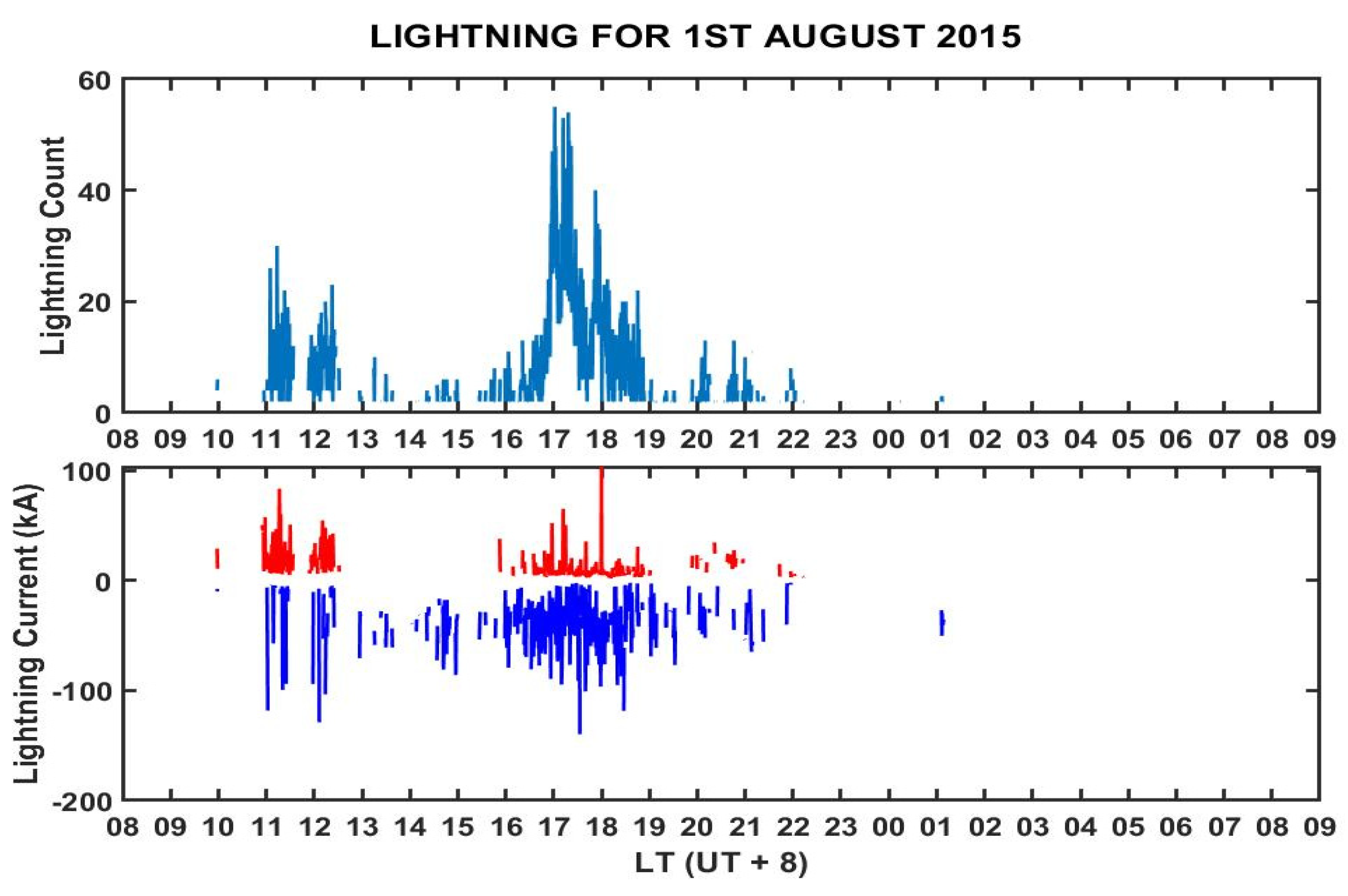
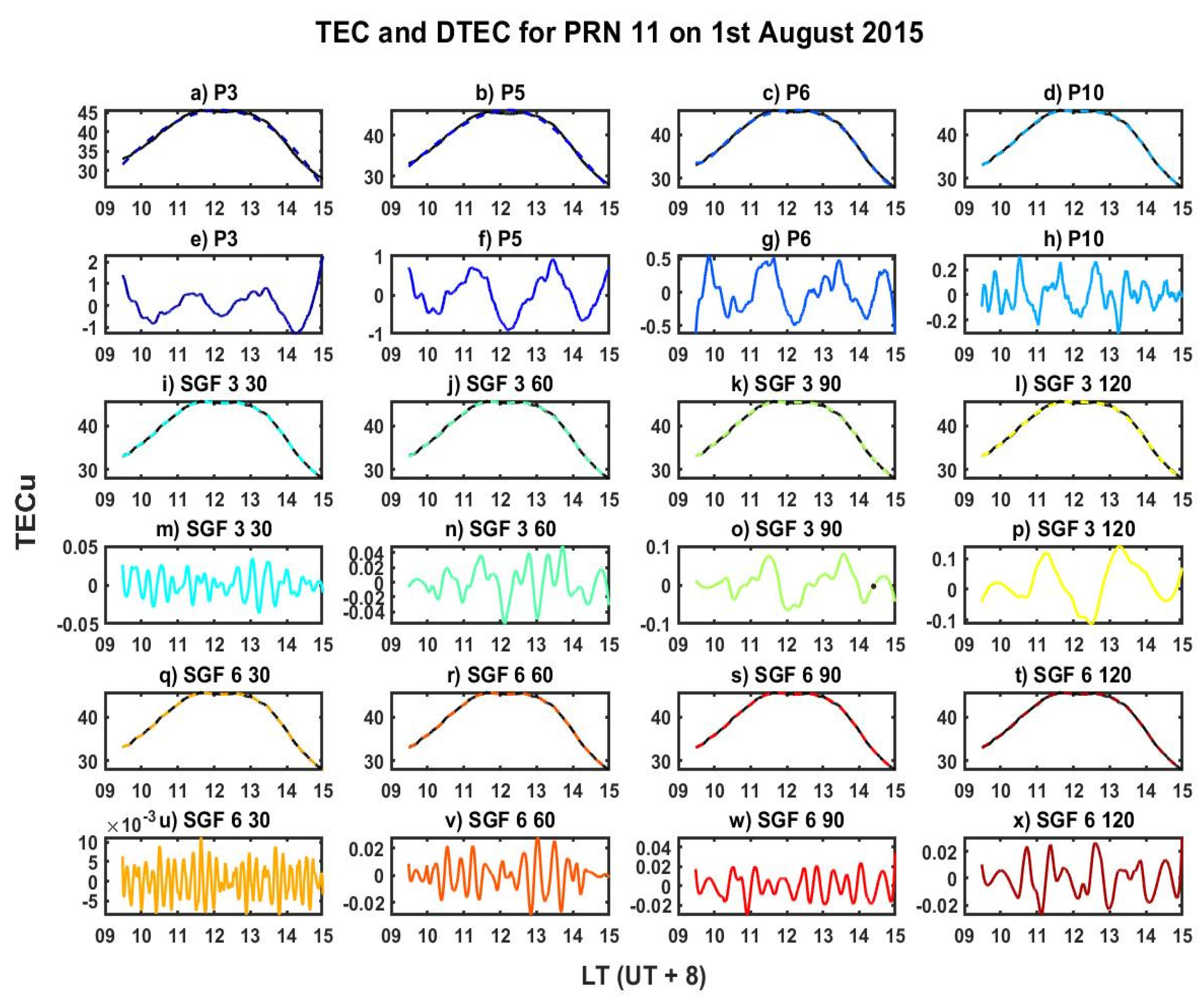
3.3.1. 1st August

This day was the first of the non-lightning days after lightning days. Few lightning counts were seen at 11–12, 16–18 and 21–22 LT. Figure 18 and Figure 19 show the lightning activity, TEC and DTEC of PRN 11.

P3, P5, P6 and P10 all had constant DTEC amplitude of ±0.2 on PRN 7, as seen in panels e to h of Figure 20 and Figure 21. The Sgf_3_and 6 parameters all had constant DTEC amplitudes. Sgfs 3_30, 3_60, 6_30, 6_90 and 6_120 had amplitudes of about ±0.02TECu, while 3_90 and 3_120 all had ±0.1TECu. All of the DTEC techniques used were able to show that this day was a quiet day, having constant DTEC amplitudes.

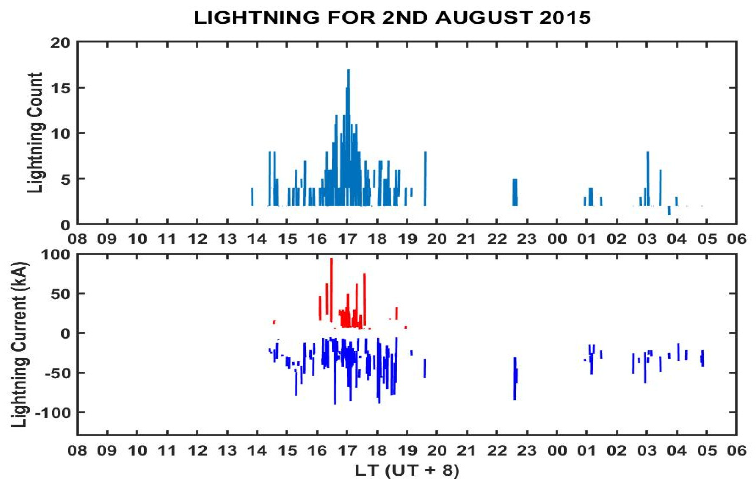
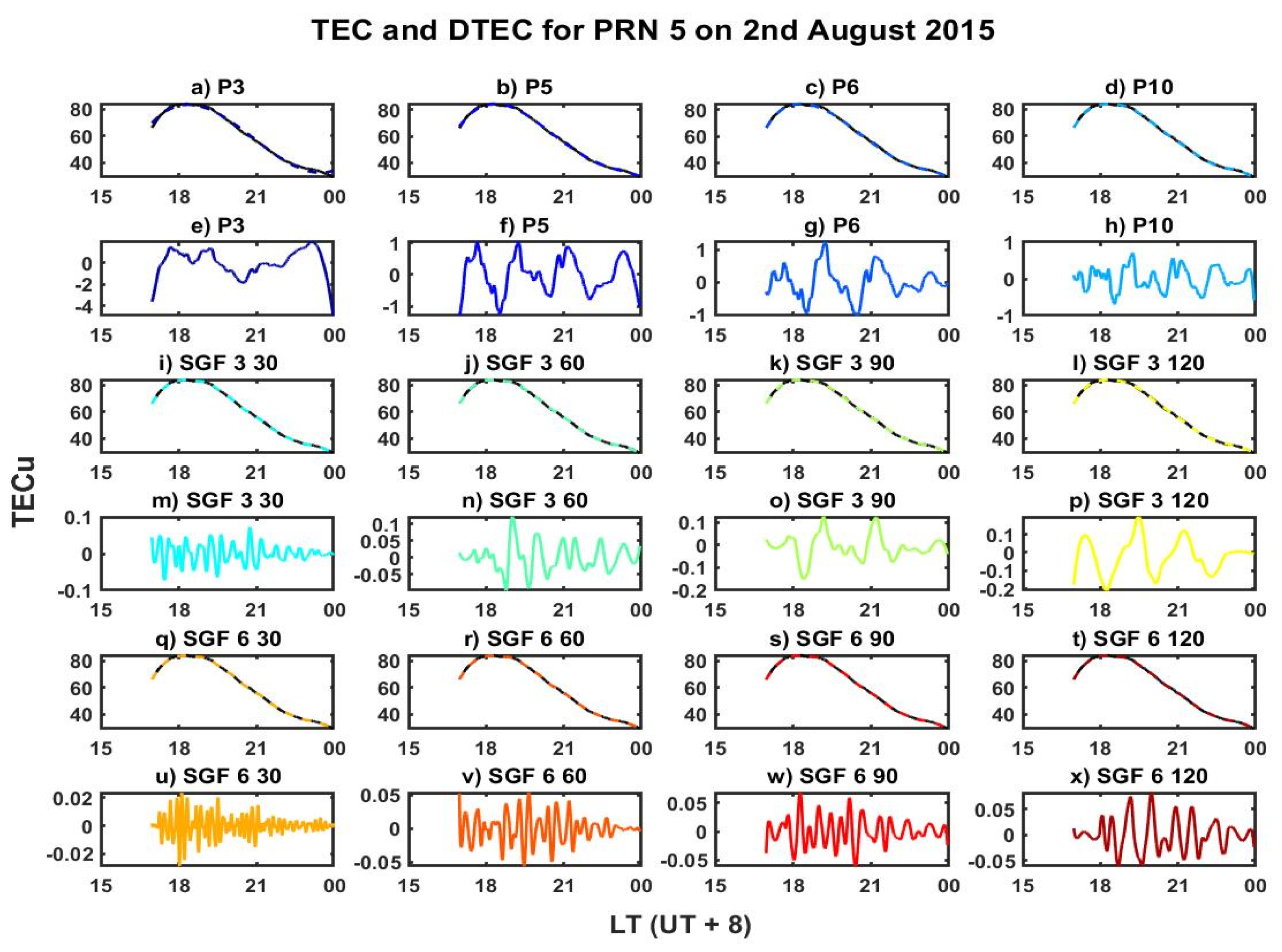
3.3.2. 2nd August

This day was the second non-lightning day after a lightning day. Figure 20 shows the lightning activity in terms of current and count. Few lightning counts are seen at 14–19 or 03–04 LT. Figure 21 shows TEC and DTEC for PRN 5.

Less useful information could be derived from the DTEC of P3 in panel e of Figure 21. P5, P6 and P10 had a constant DTEC amplitude of about ± 0.1TECu. Sgf parameters also had constant amplitude throughout. Sgf_6_30 recorded ±0.02TECu. Sgfs 3_30, 6_60, 6_90 and 6_120 recorded ±0.05TECu, while 3_90 and 3_120 had ±0.1TECu.

The constant amplitude shown by the detrending techniques indicate that this day was a quiet day.

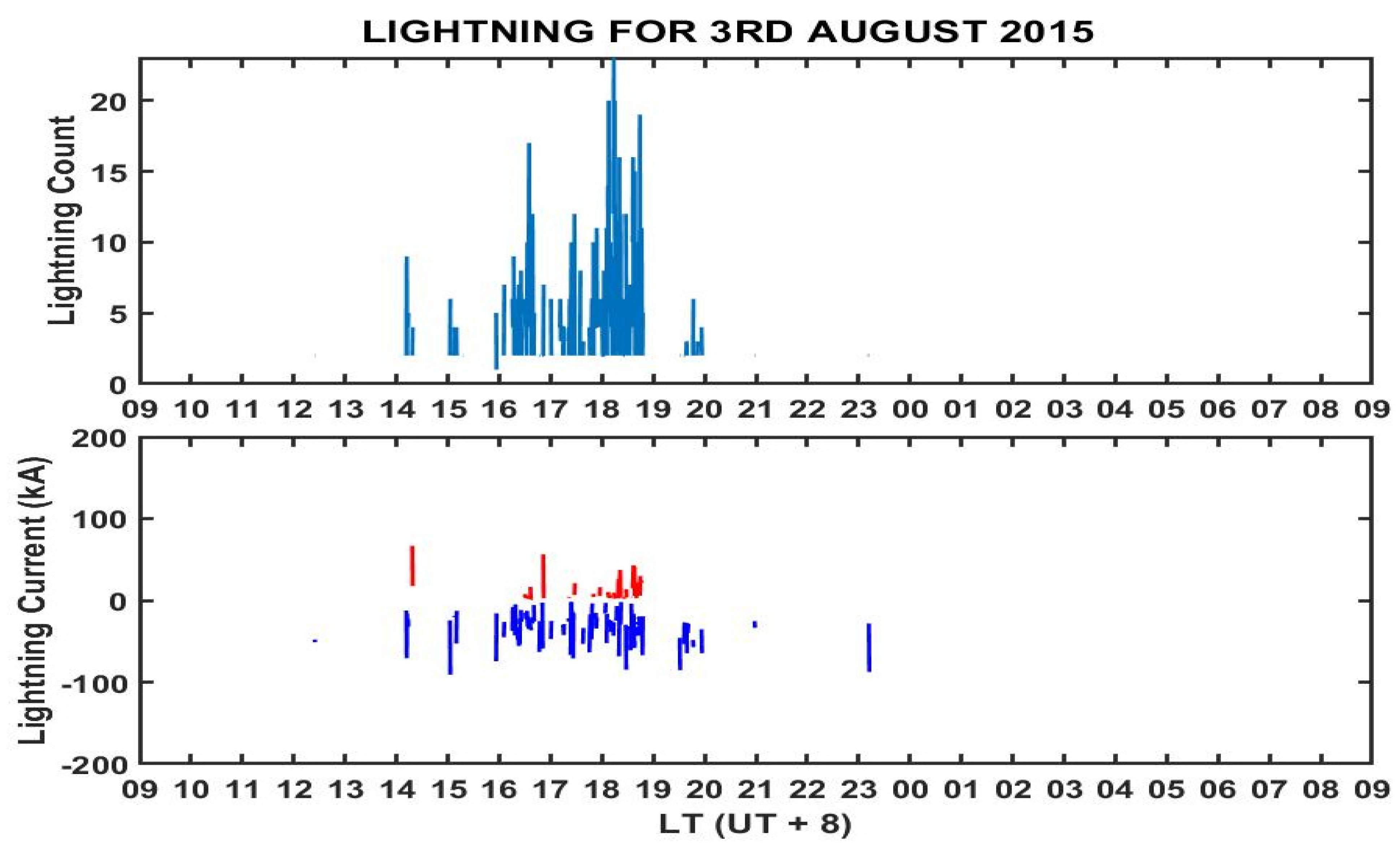
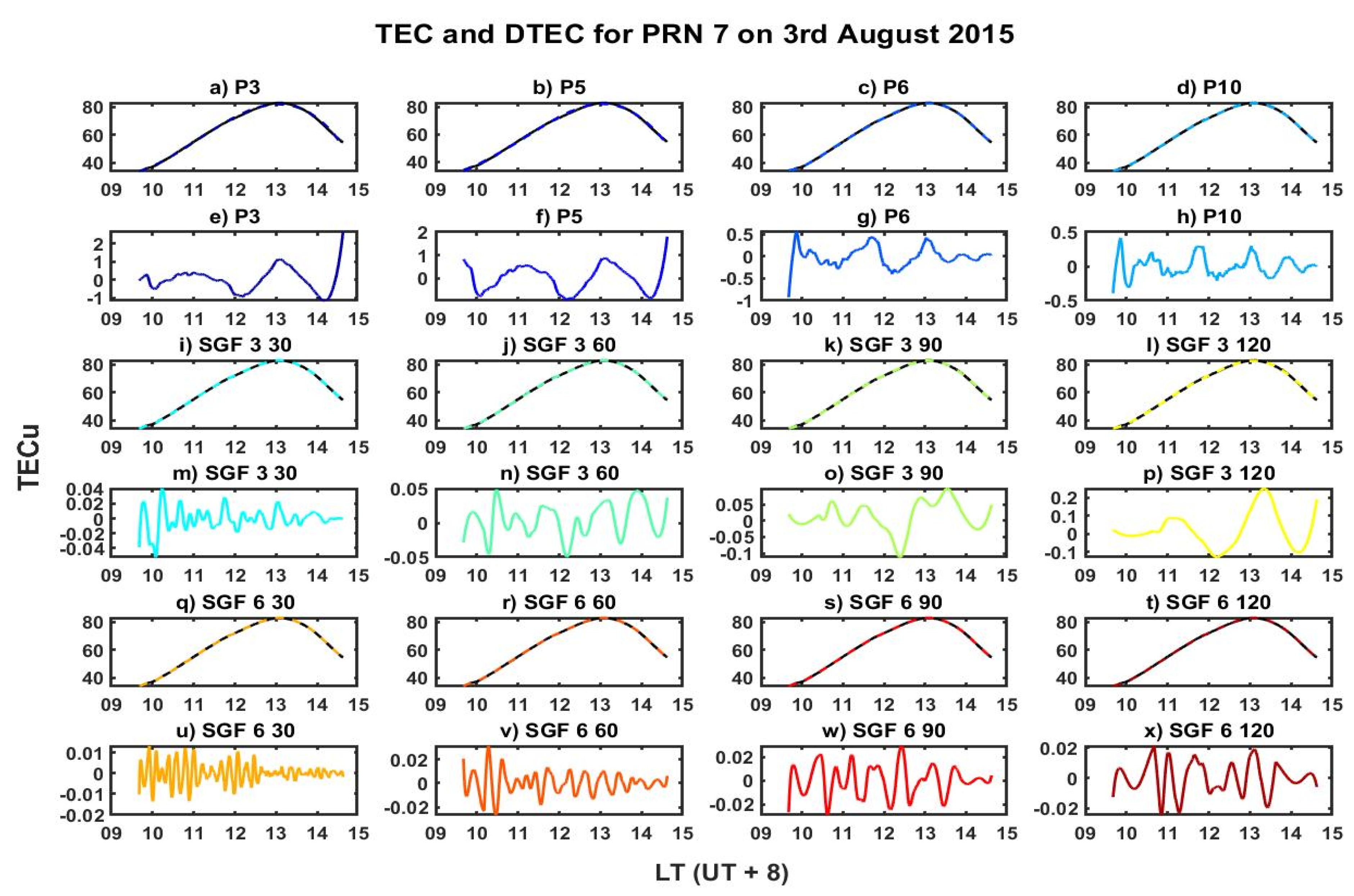
3.3.3. 3rd August

This was the last non-lightning day in the third set of days. Figure 22 shows the lightning activity for this day. Few lightning counts were seen, mostly at 14–19LT. Figure 23 show the time of passage of PRN 4 and its respective TEC and DTECs.

All detrending parameters for PRN 4 had constant DTEC amplitudes at the time of its passage. The polynomials had higher values compared to the those of sgf. The constant amplitude once again indicates that this day was a quiet a day. The amplitudes recorded by the detrending parameters were similar to those of other non-lightning days.

Table 2. Summary of which DTEC parameters could indicate non-lightning and lightning events. R means represent, D means detected, ND means not detected.

Day/DTEC Method		P3	P5	P6	P10	sgf_3_30	sgf_3_60	sgf_3_90	sgf_3_120	sgf_6_30	sgf_6_60	sgf_6_90	sgf_6_120
First set of days	9th July	R	R	R	R	R	R	R	R	R	R	R	R
	10th July	R	R	R	R	R	R	R	R	R	R	R	R
	11th July	R	R	R	R	R	R	R	R	R	R	R	R
Second set of days	17th July	D	D	D	D	D	D	D	D	D	D	D	D
	18th July	ND	ND	ND	D	D	D	D	D	D	D	D	D
	19th July	-	D	D	D	D	D	D	D	D	D	D	D
Third set of days	1st August	R	R	R	R	R	R	R	R	R	R	R	R
	2nd August	R	R	R	R	R	R	R	R	R	R	R	R
	3rd August	R	R	R	R	R	R	R	R	R	R	R	R

provides a summary of which DTEC method and parameters were able to detect lightning events on lightning days and to represent the quiet nature of non-lightning days according to the 2DC approach for the results enumerated above.

4. Discussion

From the results in Section 3 and Table 2, all of the detrending methods had individual DTEC amplitudes that were mostly the same or constant during both sets of non-lightning days at the time of passage of the satellites (panels e–h, m–p, and w–x of Figure 6, Figure 8, Figure 10, Figure 19, Figure 21 and Figure 23). Days without changes in amplitude show that the ionosphere was quiet, which truly reflects the weather events, as there were no geomagnetic storms, lightning events, or sunspots.

During the lightning days, P5, P6 and P10 could detect lightning events using the 2DC approach. DTEC amplitude increased, as seen in panels e to h of Figure 13 and Figure 17. This observation agrees with Rahmani, et al. [11] and Ogunsua, et al. [12], who used P10 and P6 respectively to detect the occurrence of lightning. The amplitude values, however, were no different from those of non-lightning days. The amplitude for non-lightning days was on average between ±0.5–5TECu. Lightning days at the time of expected DTEC changes also recorded increases in amplitude values between ±0.5–5TECu. This does not show a clear distinction between the lightning days and non-lightning days. Thus, the distinguishing condition of 2DC was not met. This non-distinction could be the reason Kumar, et al. [29] reported no difference between lightning and non-lightning days, and makes polynomials less suitable for distinguishing lightning days.

Coster, et al. [30], suggests the accuracy of DTEC is about ±0.05TECu. Any fluctuations above this could be a disturbance. The Savitzky–Golay parameters mostly had ±0.05TECu on non-lightning days and saw an increase to about ±0.06–2TECu on lightning days (panels m–p and w–x of Figure 12, Figure 13, Figure 15 and Figure 17), in agreement with this suggestion. This further suggests that the Savitzky–Golay filters were better at detecting lightning activity and representing the quiet activity of non-lightning days. Sgf_3_30, 6_30, 6_60 and 6_120 mostly had amplitudes of ±0.05TECu on non-lightning days and saw an increase to ±0.06–0.2TECu at the time of expected DTEC amplitude changes on lightning days. These parameters were therefore able to detect lightning events and distinguish lightning days from non-lightning days using 2DC. Sgf_3_90 and 3_120 had amplitudes of ±0.1TECu on non-lightning days (panels o and p of Figure 6, Figure 8, Figure 10, Figure 19 and Figure 21) and an increase to the same value at the time of expected DTEC changes on lightning days (panel o and p of Figure 12, Figure 15 and Figure 17). These two parameters, like the polynomials, could only detect lightning activity, not distinguish between lightning and non-lightning days. The time window of 90 to 120 min is the typical period of TIDs. Sgfs 3_90, 3_120, 6_90 and 6_120 being able to detect DTEC changes affirms that lightning can induce TIDs as, suggested by Mahmud M [13]. Another interesting observation can be seen in Figure 5: DTEC amplitude changes are observed on PRN 13, although 9th July was a non-lightning day. PRN 13 passed at a time about 1–2 h after the few lightning counts on 9th July, as seen in Figure 8. It could be that PRN 13 passed directly over the location of the lightning strokes, and was therefore able to detect them. This also confirms the observation by Qin, et al. [31] that even a small lightning stroke can effect changes in the ionosphere.

As the Savitzky–Golay parameters sgf_3_30, 6_30, 6_60, 6_90 and 6_120 met all the conditions in 2DC, further evaluation through statistical means was deployed to choose the most suitable parameter. Linear correlations between lightning count and DTEC on lightning days for the PRNs presented in Section 3 above were conducted. The significant level (α) for accuracy assessment was 0.05, and the correlation coefficients and p-values for each PRN are presented in

Table 3. Correlation coefficients between lightning counts and DTEC values from the various parameters during lightning days. PRNs are placed in brackets. E is the scientific notation for base ten.

	CORRELATION COEFFICIENT				P-VALUE
DTEC Method/Satellite	17th July (13)	17th July (21)	18th July (5)	19th July (15)	17th July (13)	17th July (21)	18th July (5)	19th July (15)
sgf_3_30	−0.0532432	0.212518	0.1380252	0.2172065	0.1844358	1.837E-07	6.041E-05	2.313E-09
sgf_6_30	0.0205577	0.2196998	0.3005218	0.3456595	0.6085514	6.823E-08	5.672E-19	3.204E-22
sgf_6_60	−0.0195246	0.0597396	−0.0388213	0.1613585	0.6266822	0.1469133	0.2613414	1.015E-05
sgf_6_90	0.0040953	0.5853365	0.465207	0.4095069	0.9187456	1.245E-55	2.789E-46	2.492E-31
sgf_6_120	0.34839	0.2449198	0.3050079	0.4778427	3.23E-19	1.603E-09	1.599E-19	1.554E-43

. Figure 24 shows the respective scatter diagrams of the correlations for these parameters.

From Table 3 and Figure 24, the DTEC amplitudes were mostly moderately positively correlated to lightning. The sgf_6_120 parameter was the most consistent with lightning count for all the days and PRNs, with an average moderate positive correlation of about 0.5. With such consistency and moderate positive correlation, sgf_6_120 was selected as the most suitable after meeting the conditions of 2DC. The time frame of 120 min further suggests that the disturbances could be TIDs, with lightning as the potential source. The coefficient of 0.4–0.5, though moderate, could be deemed as significant. Gravity waves in equatorial regions correlated with equatorial plasma bubbles (EPB) was 0.2. Though a weak correlation, this was consistent over a long period of time, and given the multiple sources of EPBs it should not be neglected. [32] Lightning is also a source of gravity waves [14], and a relative higher correlation of 0.4 could equally be deemed significant. The findings from the sgf confirms studies in other disciplines, such as medicine, that a Savitzky–Golay filter can represent physical parameters and events and provide detail which could otherwise be missed.

5. Conclusions

In this study, two commonly used TEC detrending methods were evaluated for the detection of lightning events in a low latitude region. The results show that a Savitzky–Golay filter of order 6 with a time window length of 120 min best detected the occurrence of lightning compared to the other parameters used in the study. The evaluation was done on the individual satellites rather than the average TEC over a station, as in some studies cited [13]. The individual satellite approach offers a better view than the average approach, as some minute details may be missed or cancelled out during the averaging. In addition, the best time frame being 120 min shows the potential of lightning to inducing TID. Further investigation is suggested in order to explore this observation.

References

- Maletckii, B.; Yasyukevich, Y.; Vesnin, A. Wave signatures in total electron content variations: Filtering problems. Remote. Sens. 2020, 12, 1340. [Google Scholar] [CrossRef] [Green Version]
- Cherniak, I.; Zakharenkova, I. Large-scale traveling ionospheric disturbances origin and propagation: Case study of the december 2015 geomagnetic storm. Space Weather 2018, 16, 1377–1395. [Google Scholar] [CrossRef]
- Ray, S.; Roy, B.; Paul, K.S.; Goswami, S.; Oikonomou, C.; Haralambous, H.; Chandel, B.; Paul, A. Study of the effect of 17–18 March 2015 geomagnetic storm on the Indian longitudes using GPS and C/NOFS. J. Geophys. Res. Space Phys. 2017, 122, 2551–2563. [Google Scholar] [CrossRef]
- Belehaki, A.; Kutiev, I.; Marinov, P.; Tsagouri, I.; Koutroumbas, K.; Elias, P. Ionospheric electron density perturbations during the 7–10 March 2012 geomagnetic storm period. Adv. Space Res. 2017, 59, 1041–1056. [Google Scholar] [CrossRef]
- Kong, J.; Yao, Y.; Zhou, C.; Liu, Y.; Zhai, C.; Wang, Z.; Liu, L. Tridimensional reconstruction of the Co-Seismic Ionospheric Disturbance around the time of 2015 Nepal earthquake. J. Geod. 2018, 92, 1255–1266. [Google Scholar] [CrossRef]
- Liu, Y.; Jin, S. Ionospheric Rayleigh wave disturbances following the 2018 Alaska earthquake from GPS observations. Remote. Sens. 2019, 11, 901. [Google Scholar] [CrossRef] [Green Version]
- Polyakova, A.S.; Perevalova, N.P. Investigation into impact of tropical cyclones on the ionosphere using GPS sounding and NCEP/NCAR Reanalysis data. Adv. Space Res. 2011, 48, 1196–1210. [Google Scholar] [CrossRef]
- Yu, S.; Liu, Z. The ionospheric condition and GPS positioning performance during the 2013 tropical cyclone Usagi event in the Hong Kong region. Earth Planets Space 2021, 73, 1–16. [Google Scholar] [CrossRef]
- Yang, Z.; Liu, Z. Observational study of ionospheric irregularities and GPS scintillations associated with the 2012 tropical cyclone Tembin passing Hong Kong. J. Geophys. Res. Space Phys. 2016, 121, 1–13. [Google Scholar] [CrossRef]
- Lay, E.H.; Shao, X.M.; Kendrick, A.K.; Carrano, C.S. Ionospheric acoustic and gravity waves associated with midlatitude thunderstorms. J. Geophys. Res. Space Phys. 2015, 120, 6010–6020. [Google Scholar] [CrossRef]
- Rahmani, Y.; Alizadeh, M.M.; Schuh, H.; Wickert, J.; Tsai, L.-C. Probing vertical coupling effects of thunderstorms on lower ionosphere using GNSS data. Adv. Space Res. 2020, 66, 1967–1976. [Google Scholar] [CrossRef]
- Ogunsua, B.O.; Srivastava, A.; Bian, J.; Qie, X.; Wang, D.; Jiang, R.; Yang, J. Significant day-time ionospheric perturbation by thunderstorms along the West African and Congo sector of equatorial region. Sci. Rep. 2020, 10, 8466. [Google Scholar] [CrossRef]
- Amin, M.M. Influence of Lightning on Electron Density Variation in the Ionosphere Using WWLLN Lightning Data and GPS Data. Master’s Thesis, University of Cape Town, Cape Town, South Africa, 2015. [Google Scholar]
- Tang, L.; Chen, W.; Chen, M.; Osei-Poku, L. Statistical observation of thunderstorm-induced ionospheric gravity waves above low-latitude areas in the northern hemisphere. Remote. Sens. 2019, 11, 2732. [Google Scholar] [CrossRef] [Green Version]
- Liu, T.; Yu, Z.; Ding, Z.; Nie, W.; Xu, G. Observation of Ionospheric Gravity Waves Introduced by Thunderstorms in Low Latitudes China by GNSS. Remote. Sens. 2021, 13, 4131. [Google Scholar] [CrossRef]
- Jardim, R.; Morgado-Dias, F. Savitzky–Golay filtering as image noise reduction with sharp color reset. Microprocess. Microsyst. 2020, 74, 103006. [Google Scholar] [CrossRef]
- Chakraborty, M.; Das, S. Determination of signal to noise ratio of electrocardiograms filtered by band pass and Savitzky-Golay filters. Procedia Technol. 2012, 4, 830–833. [Google Scholar] [CrossRef] [Green Version]
- Coster, A.J.; Goncharenko, L.; Zhang, S.R.; Erickson, P.J.; Rideout, W.; Vierinen, J. GNSS observations of ionospheric variations during the 21 August 2017 solar eclipse. Geophys. Res. Lett. 2017, 44. [Google Scholar] [CrossRef] [Green Version]
- Savitzky, A.; Golay, M.J.E. Smoothing and differentiation of data by simplified least squares procedures. Anal. Chem. 1964, 36, 1627–1639. [Google Scholar] [CrossRef]
- Ji, S.; Chen, W.; Wang, Z.; Xu, Y.; Weng, D.; Wan, J.; Fan, Y.; Huang, B.; Fan, S.; Sun, G.; et al. A study of occurrence characteristics of plasma bubbles over Hong Kong area. Adv. Space Res. 2013, 52, 1949–1958. [Google Scholar] [CrossRef]
- Tang, L.; Chen, W.; Louis, O.-P.; Chen, M. Study on seasonal variations of plasma bubble occurrence over Hong Kong area using GNSS observations. Remote Sens. 2020, 12, 2423. [Google Scholar] [CrossRef]
- Zhang, S.-R.; Coster, A.J.; Erickson, P.J.; Goncharenko, L.P.; Rideout, W.; Vierinen, J. Traveling ionospheric disturbances and ionospheric perturbations associated with solar flares in September 2017. J. Geophys. Res. Space Phys. 2019, 124, 5894–5917. [Google Scholar] [CrossRef] [Green Version]
- Afraimovich, E.L.; Kosogorov, E.A.; Leonovich, L.A.; Palamartchouk, K.S.; Perevalova, N.P.; Pirog, O.M. Determining parameters of large-scale traveling ionospheric disturbances of auroral origin using GPS-arrays. J. Atmos. Sol. Terr. Phys. 2000, 62, 553–565. [Google Scholar] [CrossRef]
- Liu, J.; Zhang, D.-H.; Coster, A.J.; Zhang, S.-R.; Ma, G.-Y.; Hao, Y.-Q.; Xiao, Z. A case study of the large-scale traveling ionospheric disturbances in the eastern Asian sector during the 2015 St. Patrick’s Day geomagnetic storm. Annales Geophysicae 2019, 37, 673–687. [Google Scholar] [CrossRef] [Green Version]
- Freeshah, M.; Zhang, X.; Chen, J.; Zhao, Z.; Osama, N.; Sadek, M.; Twumasi, N. Detecting ionospheric TEC disturbances by three methods of detrending through dense CORS during a strong thunderstorm. Ann. Geophys. 2020, 63, 667. [Google Scholar] [CrossRef]
- Shao, X.M.; Lay, E.H.; Jacobson, A.R. Reduction of electron density in the night-time lower ionosphere in response to a thunderstorm. Nat. Geosci. 2013, 6, 29–33. [Google Scholar] [CrossRef]
- Salem, M.A.; Liu, N.; Rassoul, H.K. Modification of the lower ionospheric conductivity by thunderstorm electrostatic fields. Geophys. Res. Lett. 2016, 43, 5–12. [Google Scholar] [CrossRef]
- Loewe, C.A. Classification and mean behavior of magnetic storms. J. Geophys. Res. Space Phys. 1997, 102, 14209–14213. [Google Scholar] [CrossRef]
- Kumar, S.; Chen, W.; Chen, M.; Liu, Z.; Singh, R.P. Thunderstorm-/lightning-induced ionospheric perturbation: An observation from equatorial and low-latitude stations around Hong Kong. J. Geophys. Res. Space Phys. 2017, 9032–9044. [Google Scholar] [CrossRef]
- Coster, A.; Herne, D.; Erickson, P.; Oberoi, D. Using the Murchison Widefield Array to observe midlatitude space weather. Radio Sci. 2012, 47, 1–8. [Google Scholar] [CrossRef] [Green Version]
- Qin, Z.; Chen, M.; Lyu, F.; Cummer, S.A.; Gao, Y.; Liu, F.; Zhu, B.; Du, Y.p.; Usmani, A.; Qiu, Z. Prima facie evidence of the fast impact of a lightning stroke on the lower ionosphere. Geophys. Res. Lett. 2020, 47. [Google Scholar] [CrossRef]
- Wu, Q.; Chou, M.-Y.; Schreiner, W.; Braun, J.; Pedatella, N.; Cherniak, I. COSMIC observation of stratospheric gravity wave and ionospheric scintillation correlation. J. Atmos. Sol. Terr. Phys. 2021, 217, 105598. [Google Scholar] [CrossRef]