1. Introduction
Shallow waters are among the most interesting and exploited areas on the Earth. They are accessible and have multiple uses, for example, for unique environmental observation and tourist activities, but also pose a number of technological and research challenges. They cover not only areas in the coastal zones of the seas and oceans but also inland waters, such as lakes, rivers, and artificial reservoirs. Taking into account the management and exploitation of coast zones, as well as ecology issues, it is important to know the shape and structure of the terrain, of both the sea and the shore. Thus, many techniques have been developed over the years to present topography and bathymetry in the coastal zones and shallow waters. However, these issues are still a research challenge, and as a result numerous publications with various approaches to solve them are published. Exemplary approaches have been provided in [
1] or [
2]. In this paper, we are undertaking the problem of building a digital bathymetric model (DBM) [
3] based on integrated data from novel measurement techniques on unmanned vehicles.
The traditional method of data gathering in shallow water was manual measurements with a pole. In time, with development of engineering, it was replaced by acoustic methods, first with a single-beam echosounder and then with a multi-beam echosounder. These hydroacoustic methods are presently the basis of most hydrographic works, as mentioned, for example, in [
4,
5]. They provide the most accurate results [
6], and in many research works, they became a reference for assessing other methods’ accuracy, e.g., [
1,
7]. In some works, such as [
8], the key disadvantages of these solutions were indicated, which are mostly their labor-intensive nature, relatively small coverage (in shallow waters), and relatively complicated processing of data. Thus, alternative methods of bathymetry measurements in coastal zones have been proposed, such as the photogrammetric (mostly multispectral) method and light detection and ranging (LIDAR), in both aerial and satellite approaches. Remote sensing of river depths has traditionally relied upon passive optical image data [
9]. Many studies have proven that passive optical spectrally based approaches to depth retrieval perform well in shallow waters. Examples of use of these techniques for coastal area bathymetry can be found, especially when the mapped area is large and a classical survey would be economically ineffective. They can perform well in many applications; however, there are also some disadvantages, related mostly to technological and environmental issues. Optical methods are highly vulnerable to environmental conditions, and they are able to penetrate only relatively shallow waters. Factors such as water turbidity and color or atmospheric disturbances affect the quality and availability of measurements.
In the traditional approach, based on passive optical image data, the key issue is to estimate depth from multi- or hyperspectral images, which typically involves establishing a relationship between depth and reflectance at one or more wavelengths. The most common means of calibrating such a relation is to link georeferenced image pixels to field-based depth measurements [
9]. One of the most interesting approaches presented in literature is the use of optimal band ratio analysis (OBRA) for this purpose, presented in [
10]. Other approaches are extraction of pixel values and regression of depth measurements against them [
11], some of them also taking into account light attenuation in a water column [
12]. These methods generally perform well. However, as mentioned in [
13], as the use of remote sensing techniques for mapping shallow river waters continues to expand, so must awareness of the inherent limitations of this approach. This paper shows the need for a hybrid approach combining remote sensing with field-based methods, such as multibeam echosounder surveys, to obtain thorough, complete maps of the bathymetry of large rivers.
Among other photogrammetric approaches, the most important technique is the so-called structure from motion (SfM), which allows the elaboration of a 3D model based on computation that includes camera motion. The guidelines of the National Oceanic and Atmospheric Administration (NOAA) for using this methodology for bathymetric mapping of coastal areas are included in [
14]. It was indicated in this work that the accuracy and reliability of the measurements depend on many environmental issues, such as water clarity, seafloor surface texture, and active wave breaking. Water clarity is also crucial for determining the effective measurement depth, which is usually about a few meters. In [
15], accuracy better than 30 cm for the digital terrain model (DTM) was achieved, which in the case of shallow waters fulfills IHO special order requirements. However, simultaneously, it was stated that the results show that SfM through water can be a complex proposition. It was also proved in [
6] that the quality of the bathymetric SfM is highly sensitive to flow, turbidity, and color. Other factors can also affect the development of any photogrammetric products, such as specific atmospheric conditions affecting the quality of the photo radiometry [
16]; blurs appearing on the images [
17]; water surface reflections [
18]; and sea state, sunglint, and solar elevation angles [
19]. In [
20], refraction issues are additionally raised. It is claimed that using the SfM approach for submerged areas faces additional challenges, posed by the presence of water and, in particular, the effects of refraction. In this work, a direct comparison of two methods [
21,
22] of tackling this issue is included, showing that there is minimal difference in results produced by different refraction correction procedures. Other examples of using photogrammetrical SfM for river bathymetry can be found in [
23,
24,
25]. Studies considering refraction can also be found in [
26,
27,
28].
Another example of modern systems for bathymetry measurements is bathymetric LIDAR, usually making use of green laser for bathymetric survey. However, as given in [
29], the availability of these devices is still relatively low, mostly due to high prices. Nevertheless, in some publications, this approach is presented as functional and in [
30], it is presented as an important and developmental data source for coastal areas. In [
31,
32], it is said that although LIDAR is only feasible for relatively shallow and clear waters, due to the significance of such regions there are many airborne LIDAR systems specifically developed for bathymetry. In [
33], based on LIDAR bathymetry measurements on two lakes in Poland, it was concluded that this sensor can be used for measurements in the littoral zone (up to 1.6 m), while above this depth, data can be acquired by hydroacoustic sensors. In the study case of rivers, the maximum obtained depth was 2 m [
25]. Topobathymetric LIDAR, which can simultaneously survey land and water areas, is presented as a prospective solution in [
34,
35].
Satellite technology can also be used for bathymetric survey in coastal areas. Descriptions of various techniques (optical, radar, and laser) can be found in some publications. A fine survey on the technology is provided in [
36]; the methods presented are interesting; however, they are mostly used for large areas on a world scale. Another non-obvious example is the method of indirect bathymetry calculation based on gravimetry measurements, given, for example, in [
1,
37].
Each of the methods above has its advantages and disadvantages and is suitable for various conditions and in different areas. Thus, in many studies, data from various sources are combined in a fusion process to obtain an integrated model. In some works, described, for example, in [
30], the wider concept of topobathymetry is included. A recent example is given in [
38] in the form of an updated methodology for the topobathymetry survey by United States Geological Survey (USGS). The core idea is to combine geospatial products derived from single sources in raster form. The measurements have to be preprocessed before they are combined based on prioritizing and filling gaps in data sets. In most of the research, data from acoustic measurements are combined with other data sources. In [
39], aerial photos and multispectral images are combined with a digital elevation model (DEM) from echosounder measurements based on a pixel- and object-level fusion strategy. Another approach is used in [
40], in which a lot of time was spent on preprocessing of data from various sources (echosounder, cartographic data, manual survey), which were then combined into one data set, for which a joint DEM was provided. In [
41], a raster from echosounder data is combined with a model elaborated based on IKONOS images. In [
42], geoswath bathymetry is combined with LIDAR as spatially complementary data sets, with the analysis of various interpolation methods. In [
8], acoustic measurements are combined with data from a photogrammetric survey (SfM) by an unmanned aerial vehicle (UAV). The final product is an interpolated raster with a spatial resolution that depends on the point spacing from the sampling process. For achieving a smooth transition between SfM and echo sounding measurements, each bathymetric raster is classified by its corresponding range of high-precision scanning depths. A similar approach is also provided in [
2] for combining data for a topobathymetric model. Another approach for combining acoustic and photogrammetric survey is given in [
43], where a photogrammetric survey is used for determining the coastline, while the DEM itself is prepared based on single-beam acoustic measurements.
A complex approach to the integration of data from various sources is presented in [
44], in which many databases and sources are used. The basis is the integration of LIDAR and hydroacoustic data, any gaps therein are supplemented by data from various databases, such as Electronic Navigational Chart (ENC), General Bathymetric Chart of the Oceans (GEBCO), and legacy systems. A common database is prepared, and a common DEM is created. As the input data for the model are characterized by high density, the binning minimum value (BMV) method is used for smoothing and denoising.
Unmanned vehicles are being increasingly used in many survey techniques. The main reason for and advantage of this is reducing the workload of surveyors. UAVs as the platform for photogrammetric equipment have been used, for example, in [
2,
6,
14,
45] and also for rivers, for example, in [
20,
46,
47], while a survey with LIDAR mounted on a UAV is presented, for example, in [
29]. A review of such an application can be found in [
48]. An interesting approach is also proposed in [
8,
49], where a bathymetric survey was performed with an echosounder towed by a low-level UAV. Various echosounders mounted directly on unmanned surface vehicles (USVs) are presented in research given in [
50]. In works [
2,
6,
51], the use of UAVs for photogrammetric measurements and USVs for hydroacoustic measurements has been presented. A novel and interesting approach for planning and performing an integrated mission by UAVs and USVs is explained in [
52].
The method of combining data is another component in the development of an integrated digital bathymetric model, apart from measurement techniques. In most works, the areas for various data are defined. Usually, some kind of priority is proposed for them, indicating the most reliable source (echosounder in most cases), and then the gaps are filled by data from other sources. Such an approach has been used, for example, in [
8,
40,
42,
44]. The main problem with this approach is the ambiguity in the neighboring areas, where models of different qualities (resolution and accuracy of measurement) are fused. Other problems are the necessity of cutting of overlapping areas and the ambiguity of point classification. For example, in [
8], for achieving a smooth transition between SfM and echo sounding measurements, each bathymetric raster is classified by its corresponding range of high-precision scanning depths. In some works, after the identification of areas jointly covered, a combination of input data in them is proposed. This approach is used, for example, in [
34] for LIDAR data or in [
2] for photogrammetric data. The main issue then is the way of combining data of different types. The works involving this approach are in minority, showing research potential in this area. A joined DEM can then be elaborated as one model for integrated input data set [
44] or as the integration of a few raster surface models [
38].
The development of a digital bathymetric model also involves choosing the method for interpolation, apart from the input data set. In [
38], the geostatistical empirical Bayesian kriging method is proposed for this purpose. Kriging has also been used in [
6,
40]. Triangulation, after local smoothing, is used in [
44], while the nearest neighbor method is proposed in [
8]. In [
2], three methods are analyzed, inverse distance weighted (IDW), kriging, and natural neighbor, and IDW is indicated to give the best results. In [
53], the proposal of modification dedicated to bathymetric modeling of IDW is proposed, based on bathymetric data, and in [
54], the need for big data set reduction prior to interpolation is emphasized. As seen, a variety of methods can be used for interpolation in modeling, with satisfactory results.
Most of the research focusing on issues with modeling a shallow water surface refers to sea coastal areas, leaving a void in inland areas. Additionally, modern methods should use unmanned vehicles as the most effective survey solution and data should be integrated from various sources. The most reliable is usually derived from hydroacoustic measurements, while the most popular sensor for UAVs is a multispectral camera. In this case, the SfM methodology is usually used, allowing the most effective modeling. Data sets derived from various sources should be integrated taking into account their quality, and then the final digital surface model should be developed. Following these conclusions from literature analysis, we decided to elaborate the method of developing an integrated digital bathymetric model for shallow waters, based on hydroacoustic measurements done with a USV and photogrammetric measurements made with a UAV. In both large-hydrographic-vessel and USV surveys, there is always some part of the area inaccessible for an acoustic survey. As shown in [
45], the development of the bathymetric surface in areas with no data, based on interpolation techniques, has low effectiveness and has much bigger errors compared with the surface modeled with measured data. The results from this work were the basis for performing the research on the use of UAVs to gather the data remotely in areas inaccessible for survey surface vehicles and to integrate these data with USV measurements.
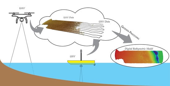
The main contribution of this study is the development of a method to combine bathymetric data acquired by hydroacoustic and optical sensors to create a digital bathymetric model for shallow water areas up to the shoreline boundary. Depending on the type of water body, these two methods have limitations related to the acquisition of bathymetric data in shallow water areas. In the case of USVs, the main restrictions are the vehicle’s draught, maneuvering capabilities in close vicinity to shoreline, submerged aquatic vegetation, and other dangerous objects (fishing nets, trees, etc.). An identified problem for UAVs is the limited possibility of using optical sensors in bathymetric measurements, which is caused by factors such as depth, water transparency, and others previously mentioned. The main research problem related to the use of photogrammetric data is the answer to the question, to what depth can these data be used to develop a digital bathymetric model? For this purpose, we propose a solution based on the creation of a bathymetric reference surface, which was developed from data acquired by a single-beam echo sounder mounted on a USV. With respect to this surface, UAV measurement points were selected based on the proposed data geoprocessing method, which were then combined with data acquired by hydroacoustic sensors. The UAV bathymetric data were developed based on a photogrammetric method using an underwater control network. In our work, we assumed that it is possible to obtain accurate bathymetric data based on SfM and an underwater control network without taking refraction into account. The final product was qualitatively and quantitatively analyzed. Based on the results, we confirmed that the assumptions (bathymetric data generation using an underwater photogrammetric network, data fusion based on a bathymetric reference surface, and dataset processing based on developed masks) make it possible to create a digital bathymetric model from hybrid data using the proposed methodology. The method was widely assessed with multivariate analysis. Various combinations of input data sets and interpolation methods were considered in the research. The measurements themselves were performed in inland waters covering shallow and ultra-shallow areas. Such a location is also unique in terms of analyzed works. However, the achieved results and the proposed method can be used for any coastal and shallow waters.
2. Materials and Methods
2.1. Study Area
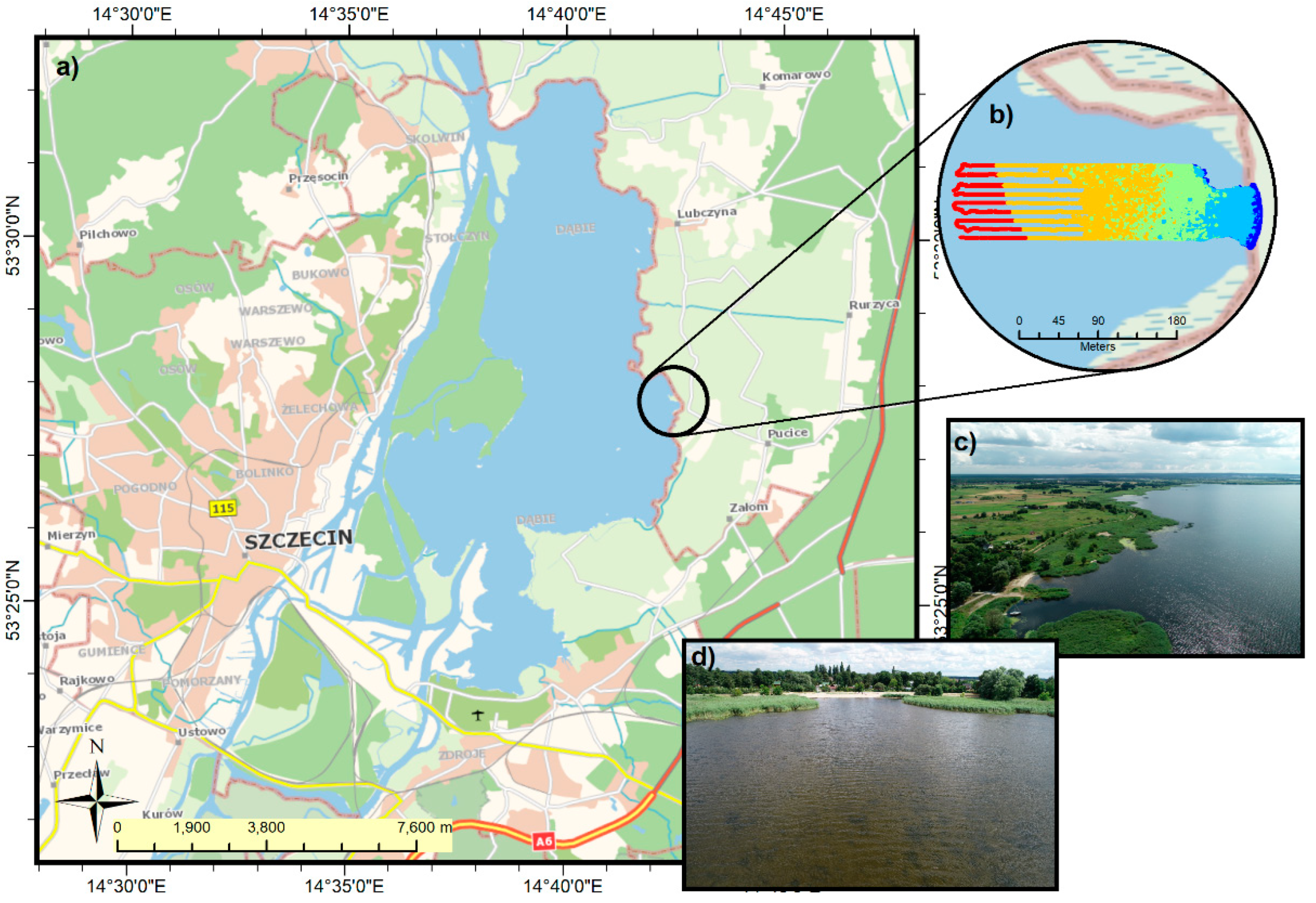
The study area is located within the village of Czarna Łąka (Poland), situated in Western Pomeranian Voivodeship, Goleniów District (
Figure 1). The study area is a part of Dąbie Lake, which is a water body with an average depth of 2.61 m [
55]. It includes a small bay with the Bystra beach. The water area from the northern and southern side is densely covered with aquatic vegetation and has a sandy beach on the eastern side. The area of the investigated water covers 0.0271 km
2 (2.71 ha). The bottom of the water area is flat for the most part, with a larger depression at the entrance to the bay. The average depth of the water area is about 1 m, and the maximum depth is 3.95 m. During the survey, the sky was slightly overcast; during the UAV flight, the sun was shining. The water surface was slightly wavy. The measurement campaign took place on 4 August 2021, between 7:30 a.m. and 1:00 p.m. UTC.
2.2. UAV Photogrammetric Data Acquisition
The photogrammetric data were acquired using an unmanned aerial system, a DJI Phantom 4 Pro quadrocopter. One of the advantages of this system is a camera integrated with a three-axis gimbal that allows recording of camera angles while taking pictures. The camera has a CMOS sensor that can take 20-megapixel images. The focal length of the camera is 8.8 mm (35 mm equivalent: 24 mm), and the field of view of the camera is 84 degrees. Images are saved in JPEG format on a microSD card. The system allows autonomous missions to be performed using dedicated software. The flight was taken from an altitude of 120 m using a basic ultraviolet (UV) filter. The UAV uses a dual positioning system: Global Positioning System and Global Navigation Satellite System (GPS-GLONASS); the positioning accuracy specified by the manufacturer for the hover is ±0.5 m vertically and ±1.5 m horizontally [
56].
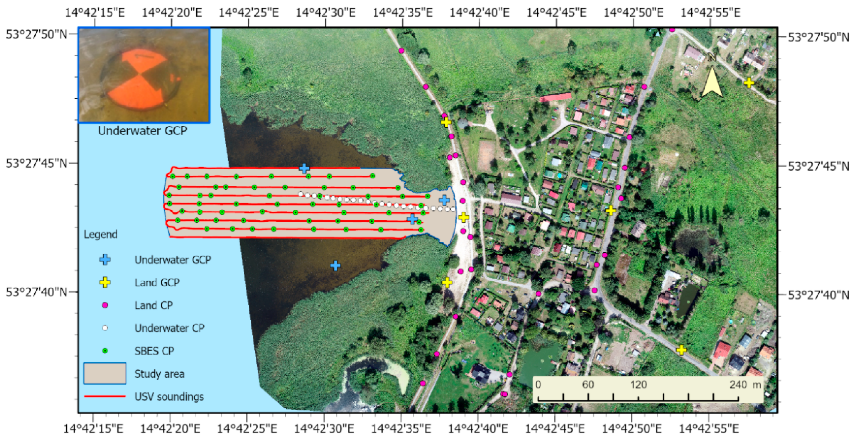
Before the flight, a temporary, signalized photogrammetric network was stabilized, consisting of 10 ground control points (GCPs): 6 on land and 4 underwater. Two types of survey GCPs were used: round white discs 27 cm in diameter (fixed with a centered surveyor’s nail) to stabilize the land survey network and orange-black survey discs 91 cm in diameter as an underwater network, stabilized with surveying pins to the lake bottom. The distribution of the network was designed during an investigation based on a field inspection. The network points were distributed evenly and on the boundaries of the survey area. The photogrammetric network was measured with a Sokkia GRX-1 receiver operating in the real-time kinematic (RTK) positioning mode.
In addition to the photogrammetric network, check points (CPs) were measured with an RTK receiver and used for height control of the DTM and the DBM. The check points for the land area were distributed evenly over the survey area, where 29 check points were measured. The underwater control points were measured as an underwater profile, where the distance of each successive point was approximately 8–9 m from the previous point; 23 such points were measured. During the flight, which lasted 18 min, 439 images in 12 stripes were acquired for an area with a coverage of 0.3207 km2. Overlap and sidelap image coverage was 85%.
Figure 2 illustrates the locations of the underwater and land GCPs, check points, USV soundings, the developed UAV orthomosaic, and the study area. In addition, a photograph of the underwater GCP is included.
2.3. USV Hydroacoustic Data Acquisition
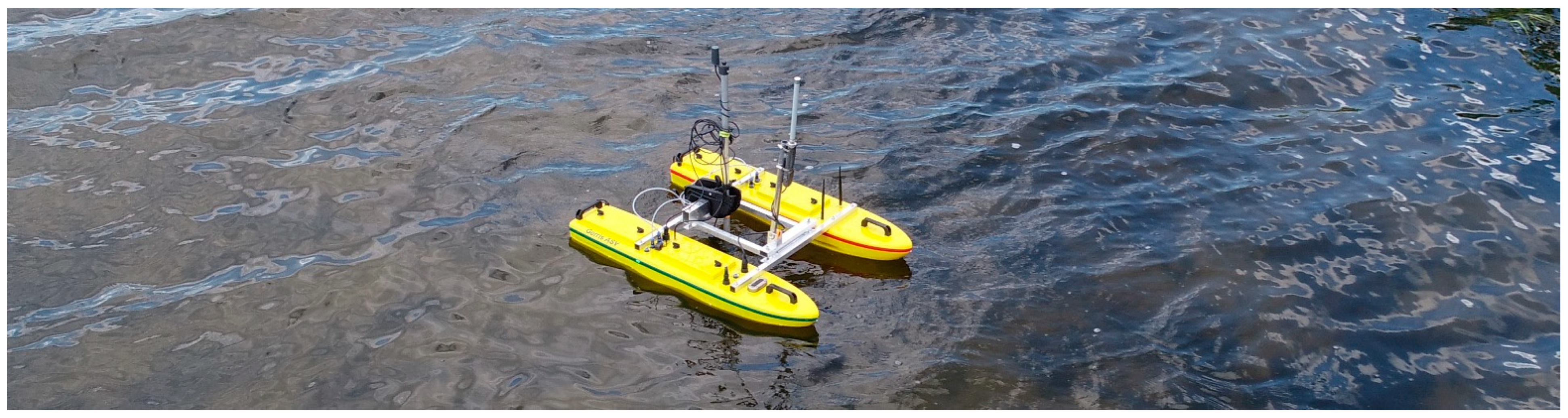
USVs are remotely operated floating platforms usually designed for surveys in extremely shallow water areas [
57,
58], where the use of standard survey boats is not viable or is risky. The Gerris ASV used within this study is dedicated to single-beam echosounder surveys. It can operate in manual and autonomous control mode on designed survey lines.
The vehicle is equipped with two electric motors driving the vehicle and a wireless radio link for control and telemetry data. The measurement system based on the Echologger EU400 single-beam echosounder and the Emlid Reach M2 RTK positioning receiver is integrated in the USV platform industrial computer. HYPACK 2021 hydrographic software is responsible for the integration of bathymetric and position data.
The echosounder transducer is mounted to the pole and connected to the industrial computer. The echosounder is equipped with an inertial measurement unit (IMU) for platform motion correction [
59]. The most important parameters of the echosounder are a high acoustic frequency and a small acoustic beam size, which affects the precision of depth measurements in shallow water areas. The GNSS receiver antenna is mounted on top of the echosounder pole. RTK corrections are provided by the Internet module via Global System for Mobile Communications (GSM). Basic parameters of the measurement system used are shown in
Table 1. Picture of USV used in the study is in
Figure 3.
2.4. Research Methodology
The research concerns full bathymetric imaging, up to the shoreline boundary, including shallow and ultra-shallow depths. Considering the operational capabilities of a USV, its range is limited by the depth of the body of water, which in the case of shallow waters, often occurring in coastal areas, makes a complete survey impossible.
In practice, other barriers, often natural, limiting the hydrographic survey can also be encountered. These may include partially submerged vegetation that creates barriers preventing a full survey, underwater obstacles, and floating vegetation on the water surface. Bathymetric data for an area inaccessible to USVs can be acquired using UAVs. Although there is some overlap between the two methods, UAV data are more heterogeneous and correct only for a certain depth, below which the values are generated with increasing errors. At a certain depth threshold value, bathymetric data cannot be acquired using the photogrammetric method due to attenuation of the electromagnetic radiation, which dissipates completely in the water, preventing it from reaching the bottom and reflecting. The magnitude of this value will be variable for a given body of water and will depend on many factors, such as water transparency, surface ripples, and bottom type and structure [
60,
61].
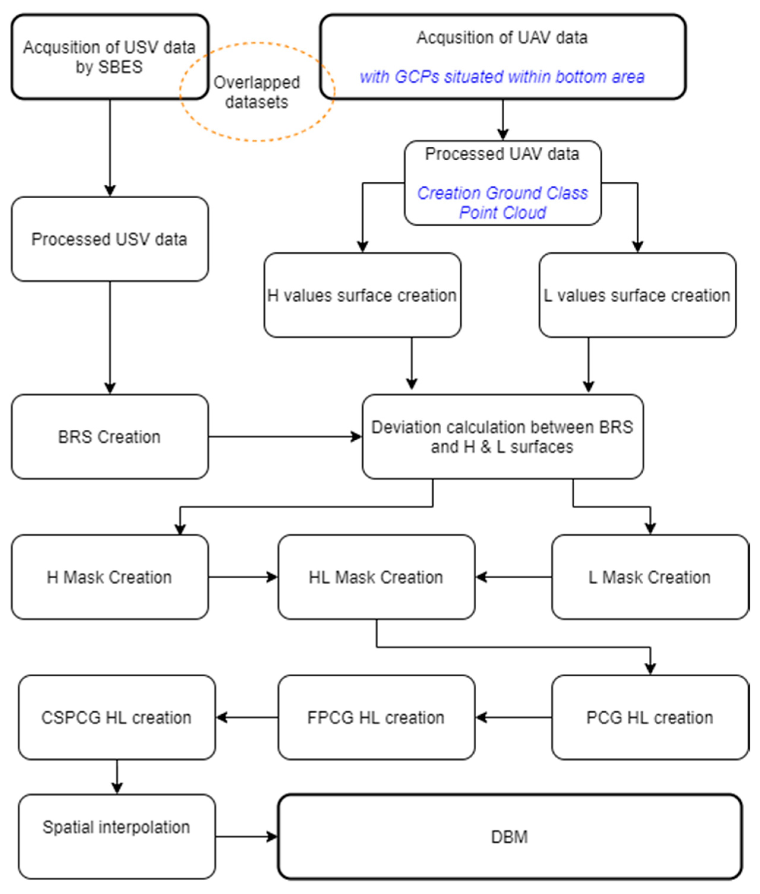
An identified problem related to the development of a unified bathymetric model is the correct integration of the data. For this purpose, research has been carried out in this paper, resulting in the development of a method to conduct this process. The main idea of the method is to create a bathymetric reference surface (BRS) from echo sounder measurements, on the basis of which, UAV cloud points are selected within an established tolerance (maximum vertical deviation from the reference surface). Such a surface was created using the triangulated irregular network (TIN) method. This surface was created to carry out multi-variate studies to create a proper UAV data set for the development of the final digital bathymetric model. The process of creating data sets from the UAV point cloud is described in
Section 2.9.
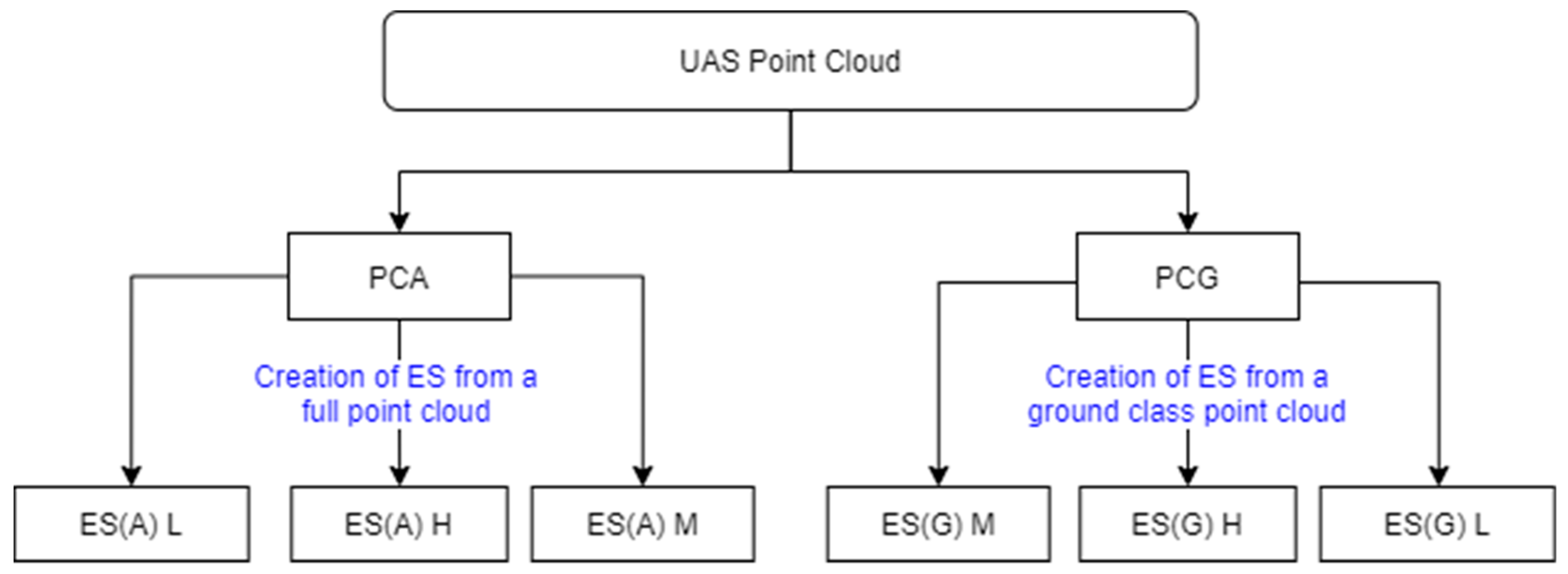
In the conducted research, a UAV point cloud (created in PIX4D Mapper) developed from all classes (PCA) and a point cloud with a ground class (PCG) were tested. Three experimental surfaces (ES) were created from each cloud in raster form. The surfaces were created using statistical map algebra operations based on individual raster cells [
62]. Each surface was created in a different way, based on the mean, the highest, and the lowest height values of the points lying within each pixel boundary. These surfaces were further used to create masks to select points in the UAV cloud based on the maximum allowable deviation from the reference surface, which we call tolerance. A mask is a polygon covering an area of the raster where the deviations from the BRS surface are contained within the tolerance limits. Four types of masks were included in the research process.
In the next stage of the research, four sets of UAV measurement points were prepared for the PCA and PCG clouds. Masks were used to create these sets, on the basis of which point selections were made in the point clouds. The result was the creation of four test sets for the PCA cloud and an analogous four sets for the PCG cloud. After analyzing the height range and finding significant deviations above the surface, additional filtering was performed on points located at heights above 0.25 m. Positive depth values were used in the final model mainly to preserve points that, due to errors in the development of the numerical bathymetric model, could be above the water surface in areas of ultra-shallow depth, on the order of a few centimeters.
The data sets prepared in this way were combined with the USV data in a single LAS format file. In the next step, digital surfaces were created for each data set using different interpolation methods. These surfaces allowed a qualitative and quantitative assessment of the created bathymetric surfaces, on the basis of which it was possible to select dedicated UAV point cloud types for merging with USV data, masks for processing point clouds, and interpolation methods in terms of creating a digital bathymetric model. The final quantitative and qualitative analysis formed the basis for discussion and conclusions. Next, the research is described in detail according to the research process adopted in the study, illustrated in
Figure 4.
2.5. USV Data Processing
Data acquisition was performed in the Hypack 2021 hydrographic software installed on the onboard computer. The operator, through a remote desktop and a Wi-Fi network, had access to all parameters and data recording status in near real time. Planning and viewing of platform telemetry parameters were performed through radio communications and Mission Planner software installed on the operator’s computer. On a background chart, the operator determined the planned route by plotting runlines. In the next stage, data acquisition, the operator supervised the progress of the mission.
All necessary corrections were applied to the single-beam echosounder system to acquire reliable bathymetric data before data recording began. Vertical and horizontal offsets were entered relative to the platform’s center reference point (CRP). The draft of the echosounder transducer was taken into account, and the average value of the speed of sound in water was included. The correctness of the entered parameters was confirmed by performing a calibration of the echosounder using the bar check method [
63]. Positioning of the platform was performed with the RTK system. For data acquisition, depth data and raw echogram data were recorded. The recorded data set from the single-beam echosounder system was processed in the SBMAX64 module of the Hypack software. First, the data from the GNSS positioning system were analyzed after data import. The trajectory of the moving surveying platform in places of temporary loss of delivered RTK corrections was corrected.
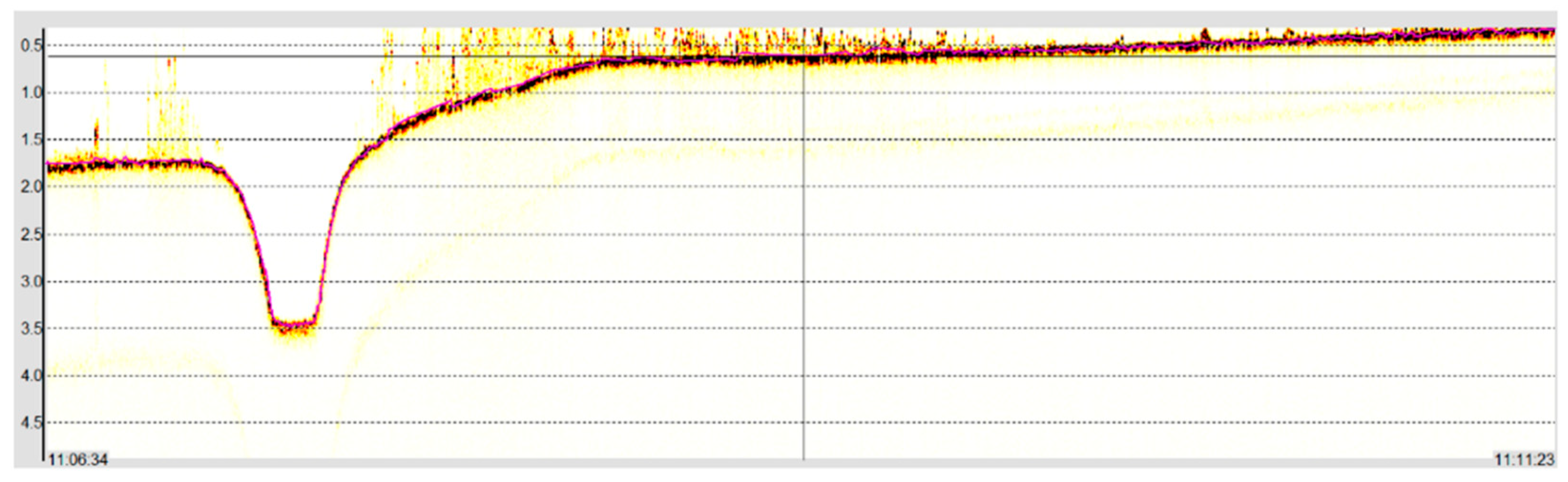
In the second step of bathymetric data analysis, manual analysis of the echograms was performed against the indications of the bottom tracking algorithm [
64] of the echosounder (
Figure 5), which is based on the amplitude of the reflected signal. Due to the heavily vegetated bottom, especially in the nearshore zone, the study required manual digitization of the echogram. The processed data set was vertically referenced to the nearest water-level gauge, Most Długi Szczecin (Długi Bridge in Szczecin). An offset for depth was implemented using the water-level gauge zero as the chart datum.
2.6. UAV Data Processing
The data acquired from the UAV platform were processed in PIX4D Mapper software (v. 4.4.12), designed for low-altitude data processing. The project was georeferenced by measuring the GCPs signalized in the field before the aerial flight and then measured on the images. A dense point cloud was created from the photographs, which was the input product for the development of the DTM. Point cloud classification was also performed in PIX4D Mapper software to separate ground points from the full point cloud. The classification is performed based on the algorithm proposed by [
65], which uses geometric and color features for the classification process, allowing each point in the point cloud to be assigned to one of six predefined classes: unclassified, ground, road surface, high vegetation, buildings, and human made object. In the software, it is not possible to select the parameters for the point cloud classification; it is only possible to choose whether the classification process should be performed (this is recommended by the developer if one of the products is to be a DTM) or whether the cloud should be left unclassified in order to build a digital surface model (DSM).
When determining the bathymetry of a water body using UAVs, a land-based survey network is usually set up [
66,
67,
68]. Other approaches are also reported, e.g., [
69] land-based GCPs are used and two buoys are placed on water for the study. Another approach is to use both land and underwater GCPs [
70]. The authors of [
70], while conducting surveys in the coastal waters of one of the Maldives islands, pointed out that the best results can be obtained using an underwater network without refraction corrections. In the present study, we used this option, taking into account the underwater photogrammetric network. Our case can be regarded as an extension of this type of research in another type of water body. The study area included inland waters with lower transparency (darker color). Another method of assessing the accuracy of the elevation models was used, measuring the CPs’ coordinates along the underwater profile.
To assess the applicability of a photogrammetric underwater network, the process of data alignment was carried out according to two independent measurement scenarios. The first measurement scenario assumed using only a land control network (6 land GCPs) for data alignment. The second scenario assumed using both land and underwater network points (10 GCPs) for data alignment.
Table 2 summarizes the results for the data georeferencing process using the two measurement scenarios described. Obtained RMSE errors for X- and Y-coordinates have values below or around a centimeter for both scenarios. The Z-coordinate for the method using land GCPs gives a smaller error, about 3 cm, while the Z error (RMS) for the second scenario gives an error of about 6 cm. In addition, errors for underwater GCPs are included, which are similar for scenario 2.
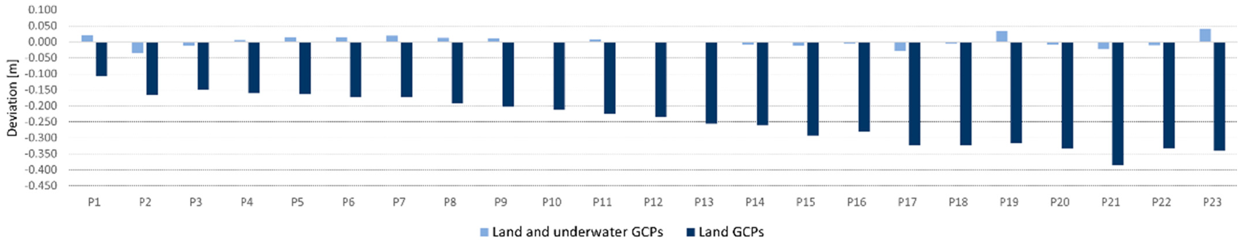
The final products obtained in the form of DTMs were checked for accuracy (height deviation) on the basis of the bottom points measured on the profile with an RTK receiver (
Figure 2).
Figure 6 summarizes the results showing the height differences on the profile obtained between these points and the height points measured on the DTM.
The minimum deviation, the maximum deviation, and the mean deviation for the survey with the land and underwater control networks were 0.00, 0.04, and 0.01 m, respectively. In a study for land GCPs only, the values were 0.11, 0.39, and 0.24 m, respectively. It should be noted that as the depth increases, the deviations for the two cases tend to increase. As an additional DTM control, an altitude check of the models on the land area was performed. The verification was performed on 29 independent control points. The minimum deviation was 0.00. The maximum deviation and the mean deviation for the study with underwater network were 0.45 and 0.05 m, respectively. For the survey without an underwater network, the values were 0.003, 0.23, and 0.04 m, respectively. Analysis of the height control points confirms the high accuracy of the developed products not only in the underwater area but also in the land area. On the basis of the above results, it can be stated that determining bathymetry by the photogrammetric method with an underwater control network without taking into account refraction correction gives good results.
2.7. Characteristics of Data Sets
In the study, it was assumed that the surface reconstruction would be carried out in the final stage using interpolation techniques. The analysis of spatial distribution and density of data is important in this case, as it may affect the accuracy of the modeled surfaces. It is especially important in the case of interpolation methods with parameters usually adjusted to the measurement set of similar or the same spatial distribution. In our case, we have a data set with varying spatial distribution and density. In the part of the body of water accessible to the USV platform, data were acquired on planned parallel profiles 10 m apart. On the profile, the data were spaced every 30–40 cm. Such a distribution can be considered as regular with a high density of equally spaced data. The situation was different for the UAV data. The data had a scattered spatial distribution with a high density per square meter, ranging from 1 to over 300 points. It should be noted here that this density was variable over the UAV data coverage area, which was related to the processing of the full point cloud. This resulted in two point clouds, the PCA cloud and the PCG cloud, with different densities. The second factor of density change was the depth, which was related to the possibility of data acquisition by the photogrammetric method. With its increase, the density of points decreased. The densities of the data are shown in
Figure 7, while the spatial distributions are shown in
Figure 8.
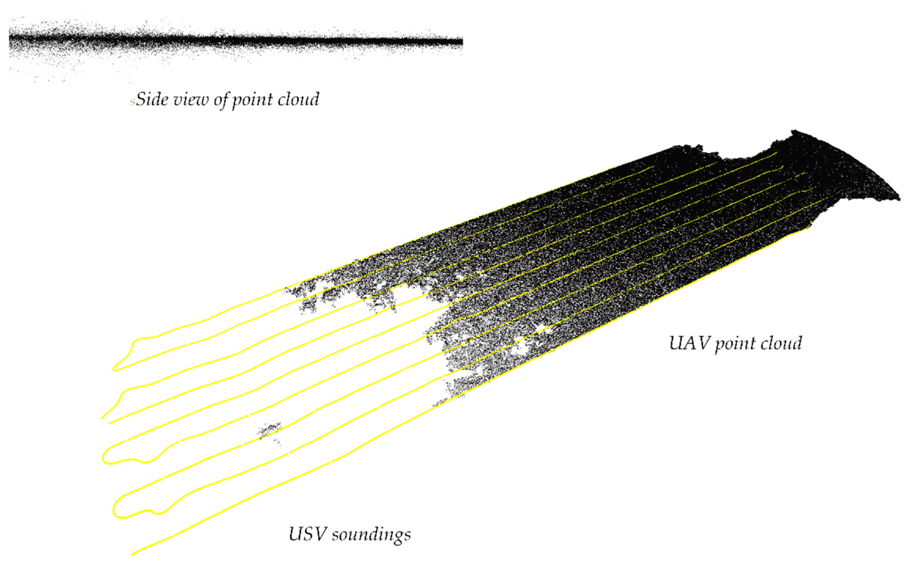
Analysis of the vertical characteristics of the data is also important, especially in terms of creating a bathymetric surface. Analyzing the data sets, it was found that USV data after processing do not have local extremes or major deviations. In the case of UAV data, the situation is different. These data are characterized by height variation, creating a layer of points. A comparison between USV and UAV data is illustrated in
Figure 8. The high roughness of the point cloud may indicate the presence of submerged vegetation, bottom microtopography, or imprecise matching of the images. It is also important to consider the way the point cloud is created, which is based on the collinearity equation and epipolar geometry, where it is important to find homologous points in at least two images. When mapping shallow water areas, it is important to take measurements under favorable conditions, such as clear water, a calm water surface, and visible bottom texture [
71], which should facilitate the acquisition of reliable height information from the point cloud. However, given the frequent variability of weather conditions during measurements and the diversity of water bodies, it is difficult to assess which parameters influence the height determination of the measurement points.
2.8. Creation of a Bathymetric Reference Surface
To carry out the surveys, a reference surface was created from the USV data, against which the deviations were calculated in subsequent steps, the motive being that bathymetric data generated from photogrammetric material have greater errors with increasing water depth, until they disappear. The second factor is that they are quite noisy. Therefore, in this case, it is difficult to determine to what depth they are generated correctly and what depth value should be taken as a reference. In the case of USV data, such a problem does not exist as the measurement is performed using hydroacoustic methods, which are recognized and proven measurement techniques. Additional recording of the echogram enables accurate processing of the depth data and removal of noise or measurement errors [
72]. It also has the advantage of recording data on profiles, which facilitates the final data processing.
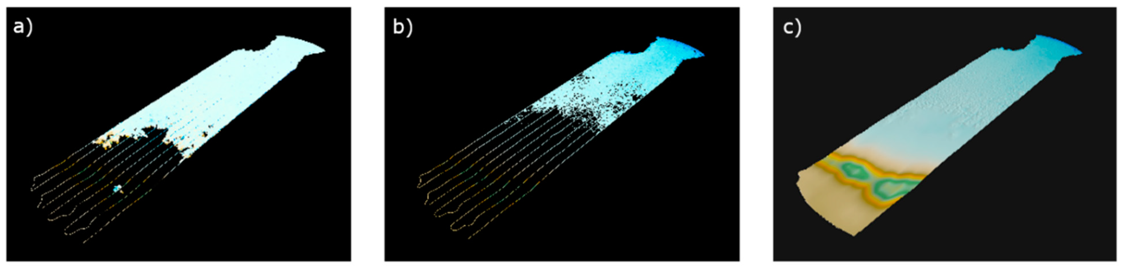
The BRS surface was created in the USV measurement point domain using the TIN method, in a GRID structure with a 0.5 m resolution. The Delaunay algorithm was used in the creation of the TIN mesh. Delaunay triangulation has the following properties: in the area of the circle described on any points of an elementary triangle, there is no other point from the whole set of measurements; it maximizes the smallest angles of elementary triangles, which makes their shape the best fit to the set of depth points [
73]. The reference surface from the USV data and the surface from the UAV data are illustrated in
Figure 9. As can be seen, the TIN surface is characterized by smoothness and continuity of the bathymetric data, while the surface created from the UAV cloud has a rough structure and generation is not possible at greater depths.
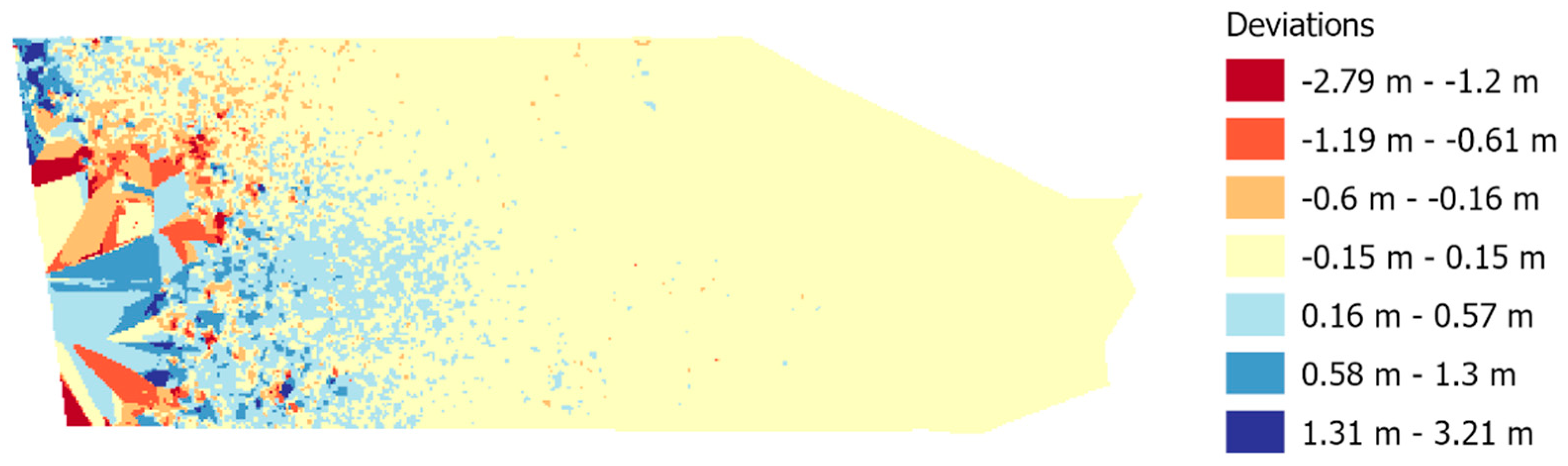
A characteristic of the bathymetric surface developed with the UAV is also that in deeper waters, the amount of erroneous data increases significantly. In
Figure 10, large deviations, both positive and negative, can be observed at these locations, ranging from −2.79 to 3.21 m.
2.9. UAV Point Cloud Processing
As mentioned earlier, low-altitude photogrammetry methods are characterized by limited possibilities for obtaining bathymetric data. Analyzing our case, we can state that the range of larger discrepancies starts from a depth of 0.7 to 1 m and the approximate limit of depth generation is 1.3 m. The purpose of this stage of data processing is to remove points from the data set that do not fall within the assumed threshold value (vertical tolerance). In this study, the threshold value was assumed at the uncertainty level for the special category area according to the IHO regulations published in Publication No. 44 [
74], which for depths of 4 m and less is 0.25 m. In the final stage of the study, eight data sets were prepared, which differed in the way that the points were removed using developed masks based on the assumed tolerance. The subsequent stages of point cloud processing are presented below.
- Stage 1:
Creation of experimental bathymetric surfaces (ES)
These surfaces were created in raster form with a resolution of 0.5 m. Rules for aggregation of points in the resulting raster cell were based successively on three statistical operations: arithmetic mean value (M), highest value (H), and lowest value (L). Surface generation was performed for both PCA and PCG clouds. Six bathymetric models were developed, denoted successively for the PCA cloud as ES(A) M, ES(A) H, and ES(A) L and for the PCG cloud as ES(G) M, ES(G) H, and ES(G) L. The data processing is illustrated in
Figure 11.
- Stage 2:
Calculation of deviations from the BRS
The operation was carried out using raster algebra tools, subtracting successive rasters of experimental surfaces with M, H, and L values from the cell values of the reference surface raster. The result of this operation was a raster with deviation values. The task was carried out using ArcGIS Pro software.
- Stage 3:
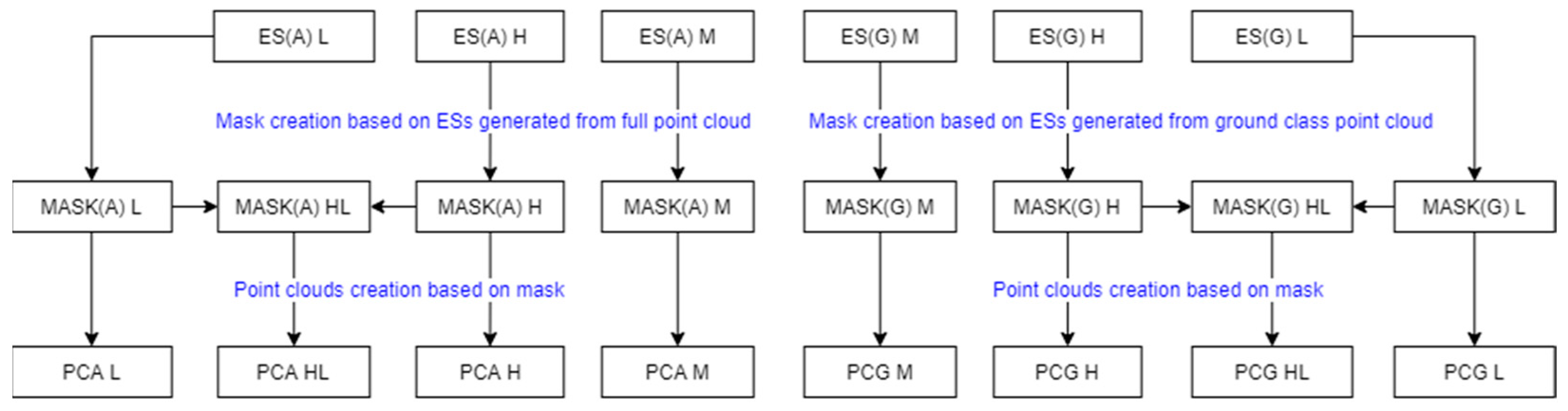
Creation of masks
Rasters with deviation values were the basis for determining the set of pixels with acceptable deviation values. These ranges were determined using the quantization method, setting two threshold levels for raster pixels: +0.25 and −0.25 m. The determined raster area based on pixels with acceptable deviations was used to create masks with M, H, and L values. One more mask type, HL, was included in the study, which was a common part of H and L masks. The motivation for its creation was that the resulting pixel in this case had to meet a threshold condition for both maximum and minimum values. In the final stage, four masks were created based on ES(A) surfaces, MASK(A) M, MASK(A) H, MASK(A) L, and MASK(A) HL, and four masks based on ES(G) surfaces, MASK(G) M, MASK(G) H, MASK(G) L, and MASK(G) HL.
- Stage 4:
Processing of point clouds using masks
The PCA and PCG clouds were processed using masks, which finally enabled the preparation of eight sets of UAV points: PCA M, PCA H, PCA L, PCA HL, PCG M, PCG H, PCG L, and PCG HL. The points contained by the corresponding mask were preserved in the geodata sets. This process is illustrated in
Figure 12.
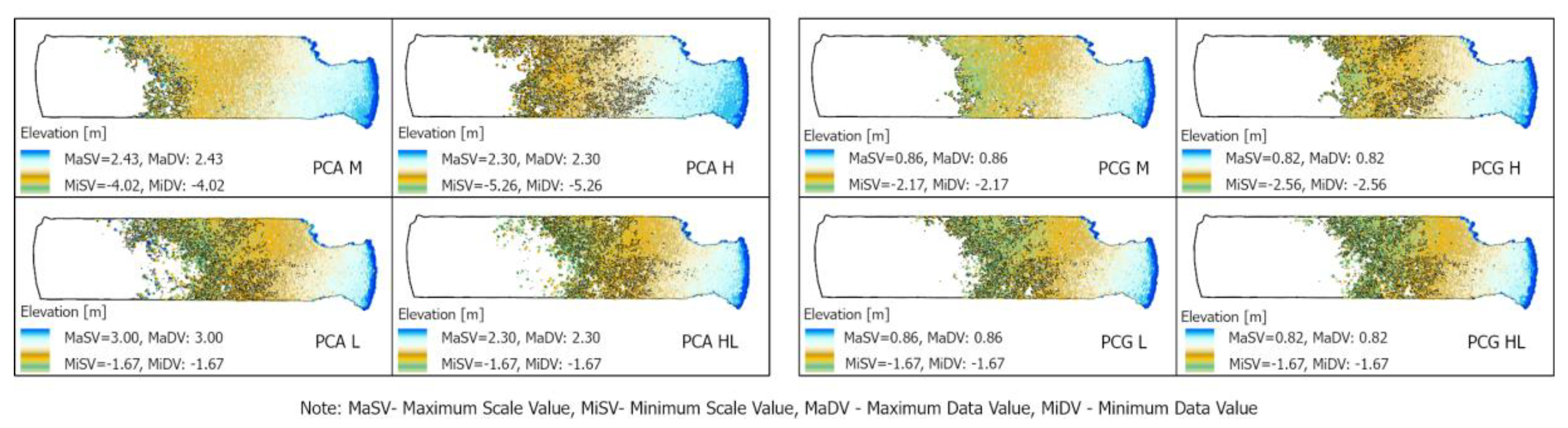
The masks and the processed sets of PCA and PCG points are illustrated in
Figure 13. As observed, a smaller depth spread was obtained for the PCG cloud, which is related to the creation of ES from ground class points only.
- Stage 5:
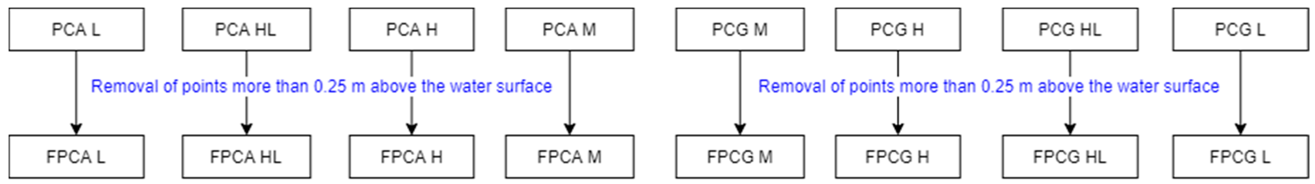
Filtration of points
The next step was to analyze points above the water level. The height of the water level was determined by referencing to a water gauge (a hydrographic reference was used). For photogrammetric surveys, water surfaces generate noise in the form of points above their surface. These were reduced in the proposed data processing. The threshold filtering value for such points was set at a predetermined tolerance of 0.25 m, the aim being to preserve points that are part of the bathymetric surface but may be above the water surface due to a model elaboration error in the z-axis. This approach allows the continuity of the model to be maintained without removing points above the water surface in ultra-shallow parts of the water area. In addition, a higher number of such points were observed near the shoreline. The reason for this is, in most cases, the problem of spectral separation of the water boundary and the presence of organic objects (e.g., sediments of dead vegetation) that accumulate there due to the wave impact. A schematic of this data processing step is shown in
Figure 14. The prefix F in front of the point cloud names denotes the data set with the points above the water surface removed according to the assumed criteria.
Figure 15 illustrates the spatial distribution of points above the water surface. As can be seen, the mask created from the mean values, MASK(A) M, leaves most such points. Significantly fewer points of this type remain for PCG clouds. An interesting observation is that for two types of point clouds, PCA and PCG, masks of H and HL type do not leave such points in the BRS surface domain. Quite a number of such points, however, can be observed in a narrow strip of the shoreline, although in most cases, their deviations from the water surface do not exceed 3 cm.
- Stage 6:
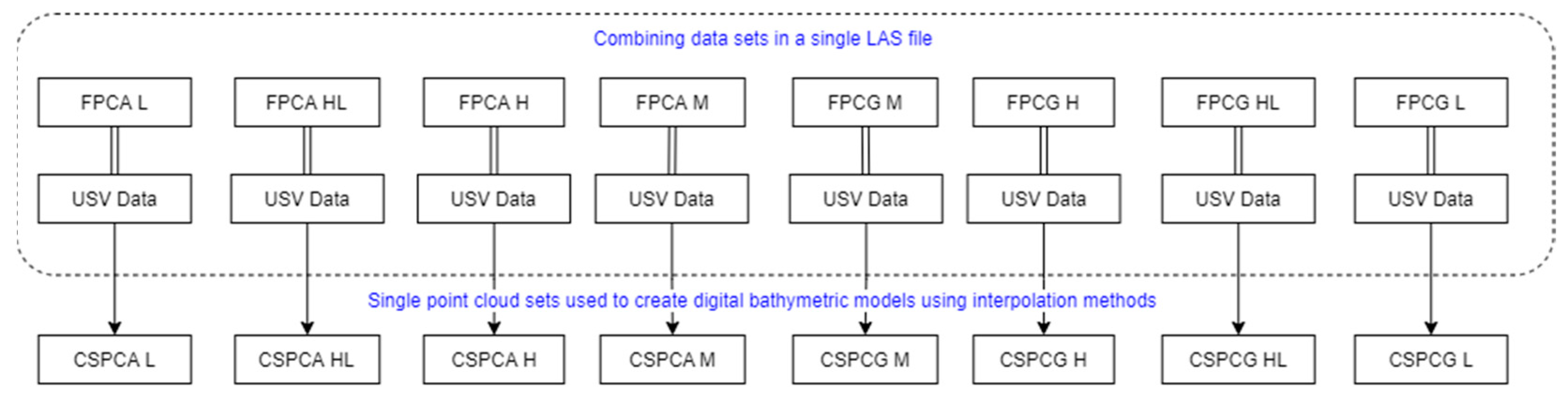
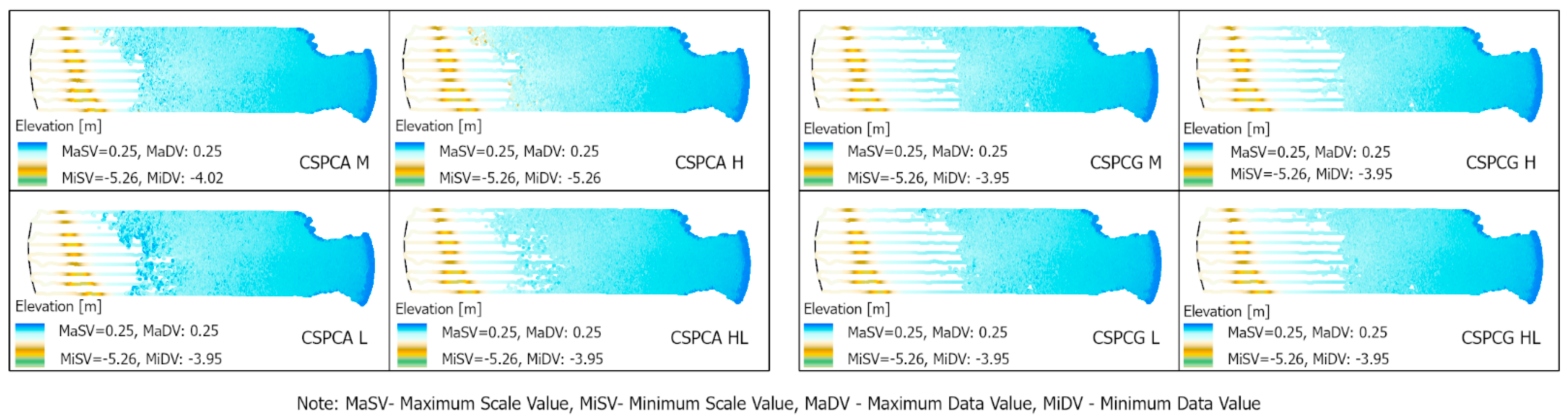
Merging data in a file
To create a single file integrating data from the two sensors, the USV data were converted to LAS format and merged with the UAV data set in Global Mapper software (v.21). The input photogrammetric data sets were FPCA and FPCG point clouds, into which the USV bathymetric data were imported. The final result was eight combined sets (CSPCA and CSPCG), which are the material for creating digital surface models by interpolation methods. The scheme for merging the data sets is illustrated in
Figure 16, while the final data sets are shown in
Figure 17.
2.10. Creation of Digital Bathymetric Models Using Interpolation Methods
The combined sets of USVs and UAVs data were used to model the surfaces using different interpolation methods. Five interpolation methods were tested: triangulation (TRI) [
75], natural neighbor (NAN) [
76], inverse distance to a power [
77], kriging (KRI) [
78], and radial basis function (RBF) method [
79]. Considering the complex spatial structure of the geodata, consisting of regular survey profiles and a point cloud with a high density and scattered distribution, this case was also included in the research. The first two of the mentioned methods are parameter-free methods, while the others require them. From the operator’s point of view, the parameter-free methods are certainly a better choice, as they do not require knowledge of the influence of parameters on the final shape of the modeled surface. This advantage can also be considered as a disadvantage because parameters usually allow for a better fit of the model to the real surface. In contrast, methods with parameters require the knowledge of parameters and an assessment of their influence on the final shape of the model. Due to the multivariate nature of the research carried out in this study, the influence of the values of various parameters of such methods, such as kriging, IDW, and RBF, was not analyzed, but the default values were used. The study of these parameters can be a further development of the research undertaken in this paper. The method parameters used were as follows: IDW power = 2; KRI, linear semi-variogram model, point kriging type, polynomial drift order = 0; and RBF, kernel type multiquadric, shape factor (R2) calculated according the formula (length of diagonal of the data extent)2/(25 × number of data points). IDW, KRI, and RBF methods used a four-sector search, 12 points per sector, resulting in interpolations from a total of 48 measurement points. The four-sector search divides the GRID mesh node space into four equal sectors with an opening angle of 90°, which makes it possible to select samples for interpolation evenly distributed around it. The usefulness of this way of searching samples was indicated in the work [
45]. Modeling was carried out in Surfer 20 software.
Figure 18 illustrates the basic steps involved in processing USV and UAV data.
3. Results
3.1. Qualitative Analysis
To perform a qualitative analysis considering the influence of all completed operations on the final surface models, a scheme was developed and is presented in Steps 1–5.
Evaluate interpolation methods for their ability to filter out points above the water surface.
Select a data set (CSPCA or CSPCG) with better visual effect.
Select the best interpolation method(s) on the data set selected in Step 2.
Select a mask based on the conclusions of Steps 2 and 3.
Return to Step 1 and apply Steps 2, 3, and 4 to the second data set rejected in the first approach.
As interpolation methods are also considered as filtering methods, in a first step, the possibility of filtering points above the water surface was analyzed. Two cases were considered: the occurrence of positive depth values in the BRS surface domain and that in the shoreline area. In the case of the BRS surface domain, CSPCA points above the water were observed for mask M and L. After the modeling process, it was found that the natural neighborhood method and the IDW method coped with this problem for mask M. In the case of a cloud formed from a class of ground-type points (CSPCG), no points above the water surface were observed in the BRS domain area for all cases and methods except for the RBF method. In contrast, a few positive values were observed near the shoreline for both cases. The percentage of pixels with positive values is summarized in
Table 3. As seen, with the exception of the RBF method, they represent a small percentage of the total area. For CSPCA sets, they range from 0.04% to 0.12%. For CSPCG, these values range from 0.04% to 0.07%. Considering this criterion, the use of the CSPCG cloud is preferable.
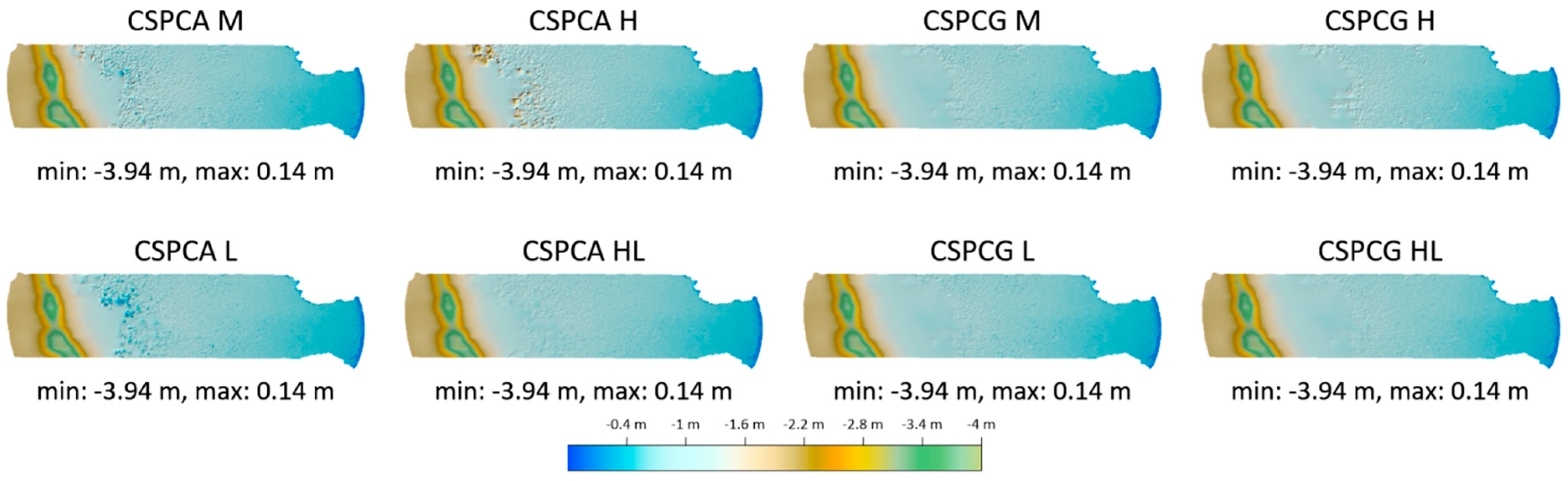
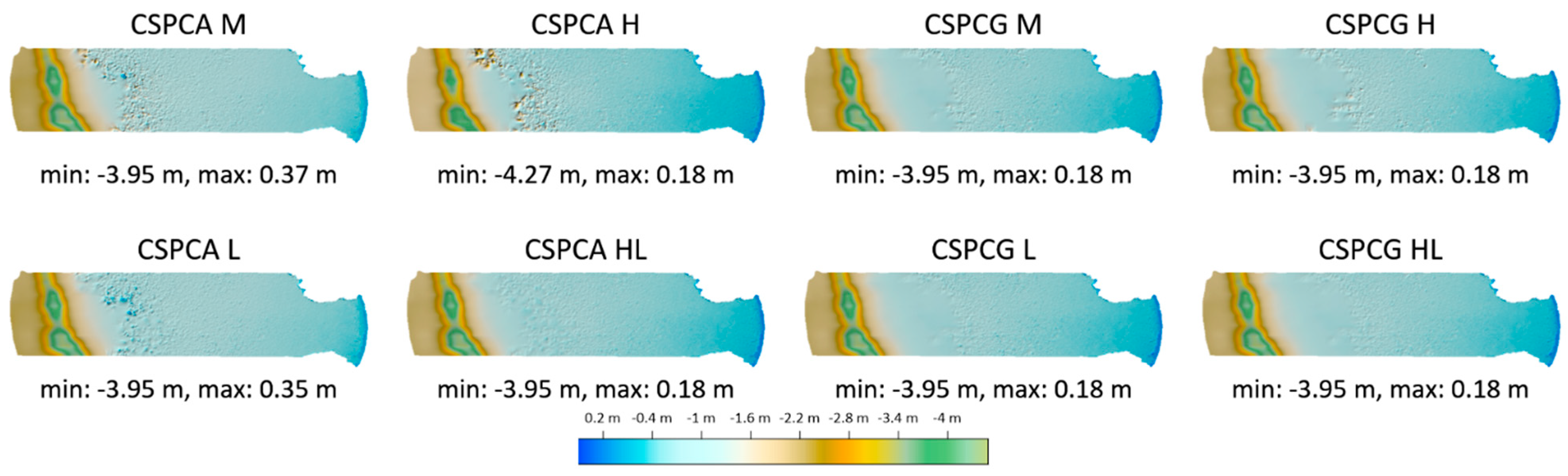
For the CSPCA data set with regard to the choice of interpolation method, the surfaces obtained with the RBF method do not give satisfactory results, while the other interpolation methods tested (KRI, IDW, TRI, and NAN) allow one to obtain qualitatively similar models with correct plasticity, which we define as the visual reasonableness of the generated surface shape, without the occurrence of local distortions or other artefacts. The use of L and H masks results in rough surfaces, while the use of the HL mask results in the smoothest surfaces. Mask M provides slightly better results than masks L and H, but worse than mask HL. The use of this mask with the IDW method provides a model with reasonably good plasticity of the terrain with a small amount of roughness.
The CSPCG data set helps obtain surfaces with a largely uniform structure. Considering interpolation methods, the best surfaces are obtained for kriging, triangulation, and IDW methods. The models obtained with these methods are similar in terms of quality. Surfaces obtained using the NAN method produce correct models, but the terrain plasticity at the interface between USV and UAV data is characterized by low smoothness. The RBF method visually produces the roughest surfaces. Analyzing the use of masks, the best visual surfaces for each of the selected methods are given by the HL mask, although the M and L masks also help achieve a satisfactory final effect of the modeled surfaces.
When analyzing the correctness of the surface reconstruction in the area covered by USV measurements (profiles), the quality was comparable for all methods. In the case of the IDW method, a tendency toward a slight curvature of the surface along the profiles was observed. However, this method preserved the highest real depth, of 0.95 m, and the positive values of height had the lowest value (0.09 m).
In conclusion, the HL mask can be considered the most effective, as it allows the correct representation of surfaces derived from both CSPCA and CSPCG clouds. The visual evaluation also concluded that creating models using CSPCG point clouds reduces the extent of UAV points used while increasing the extent of USV points. Considering the criterion of minimizing the number of pixels above the water surface, the IDW method performs the best.
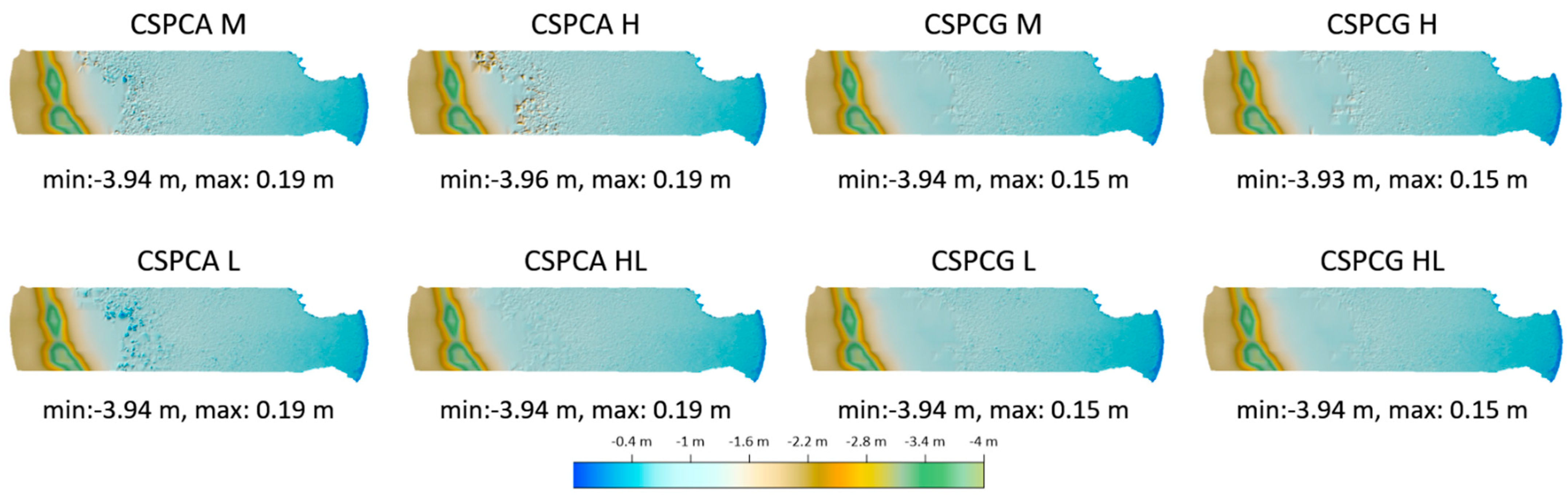
Figure 19,
Figure 20,
Figure 21,
Figure 22 and
Figure 23 show the final models obtained from the CSPCA and CSPCG data sets using the masks M, H, L, and HL. The minimum (min) and maximum (max) values were presented additionally.
Figure 19,
Figure 20,
Figure 21,
Figure 22 and
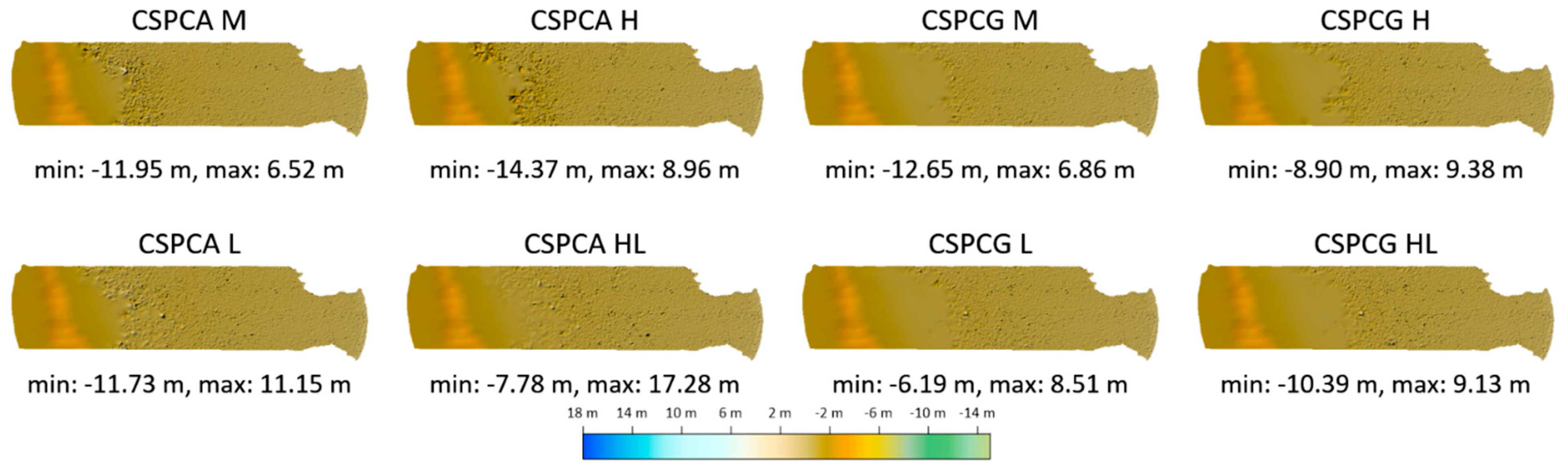
Figure 23, respectively, show the models for the methods triangulation, natural neighbor, inverse distances, kriging, and radial basis functions. In
Figure 23, due to the large local extrema generated by the RBF method, the digital bathymetric model is in the brown color range.
3.2. Quantitative Analysis
Quantitative analysis was performed using points extracted from the USV survey data set, which included 56 points, distributed evenly across the test area. For the quantitative analysis, the methods chosen were IDW, KRI, NAN, and TRI, which allow correct surface reconstruction. For each generated surface from the test data set, the difference between the heights of the test points and the corresponding points located on the surfaces of the developed digital surface model was calculated. The maximum error (MaxE), the minimum error (MinE) and the mean error (ME) were calculated for each analyzed case according to Equation (1):
where
Zi is the height measured at the CP
i point with coordinates (
xi,
yi),
zi is the height of the modeled surface at the point with coordinates (
xi,
yi), and
n is the number of
CP points.
To assess the precision of the tests carried out, the root mean square error (RMSE) was also calculated according to Equation (2):
The results are presented in
Figure 24. Analyzing the MaxEs, the worst results are obtained for the model interpolated with the IDW method created on the CSPCA data set and the H mask (0.57 m). High MaxEs are also obtained for all interpolation methods for models created from CSPCA data set using H mask (0.48–0.57 m). Better results are obtained for models from this set for mask M, where the biggest error, for the IDW method, is 0.17 m and the lowest, for the NAN method, is 0.16 m. The use of the HL and L masks and the IDW, KRI, TRI, and NAN interpolation methods decreased the MaxEs, which are in the range of 0.09 to 0.12 m. The MaxEs for the CSPCG data set for KRI, IDW, TRI, and NAN, regardless of the mask, in the range of 0.11 to 0.16 m. The smallest error for this data set is obtained for the KRI and TRI methods using the HL and L masks (0.11 m).
Analyzing the MinEs, the worst results are obtained for the model interpolated with the KRI method created on the CSPCA data set and the L mask (−0.48 m). High MinEs are obtained for all interpolation methods for models created from CSPCA data set using L mask (−0.48–−0.46 m). Better results are obtained for models from this set for mask M, where the biggest error, for the KRI method, is −0.27 m and the lowest, for the IDW method, is −0.16 m. The use of the HL and H masks and the IDW, KRI, TRI, and NAN interpolation methods decreased the MinEs, which are in the range of −0.04 to −0.06 m. The MinEs obtained using the CSPCG data set for KRI, IDW, TRI, and NAN, regardless of the mask, are in the range of −0.04 to −0.13 m. The smallest error for this data set is obtained for the IDW, NAN, and TRI methods using the H mask and IDW using the HL masks (−0.04 m).
The MEs obtained for the CSPCA data set are comparable and are in the range from −0.01 to 0.04 m. For HL and L masks, their values are the smallest and for all methods and are in the range of 0.01 m to −0.01. The MEs for the CSPCG data set are smaller, ranging from 0.01 to 0.02 m, where the best masks for all methods are L and HL (0.01 m).
The value of the RMSE is the largest for the CSPCA data set (0.12 m) for the IDW method and the H mask. The smallest RMSE values (0.03 m) for this data set are obtained for all methods (IDW, KRI, NAN, and TRI) for the HL mask. For the CSPCG data set, the maximum value of the RMSE is 0.05 for the TRI interpolation method and M mask, while the smallest values (0.03 m) are obtained for HL mask and each interpolation method tested and L mask for the IDW and KRI method.
Analyzing the MinEs and MaxEs, it can be concluded that they are comparable. The largest values of these errors for CSPCA datasets are in the range of −0.48 and 0.57 m and for CSPCG datasets are in the range of −0.13 and 0.16 m. Values for these errors, which are within the accepted tolerance (+/−0.25 m), were obtained for the CSPCA HL dataset and all CSPCG datasets. For the above cases they are between −0.13 and 0.16 m. In the case of ME for all options, the values are also comparable, which are in the range of −0.01 to 0.04 m. The lowest values were achieved for all methods for CSPCA HL dataset (0.01 m), CSPCA L dataset (−0.01 m), and for all methods for CSPCG datasets (0.01 m). However, by analyzing the RMSE, it can be concluded that by far the best results can be achieved for the CSPCG dataset for HL mask for all methods (0.03 m), L mask for IDW and KRI (0.03 m), and the CSPCA for the HL mask (0.03 m). Based on the results obtained, it can be concluded that the most universal mask for all methods is the HL mask.
4. Discussion
More and more studies are being conducted in shallow water areas. This is linked to technological development and the creation of unmanned platforms that can perform measurements in areas previously inaccessible to larger hydrographic units. However, even a small submersion of these units does not eliminate the problems associated with the survey of shallow and ultra-shallow waters. Remote sensing techniques, such as bathymetric LIDAR, and passive optical imaging methods, can be used for the tasks of mapping bathymetry to the boundaries of the coastline. In the first case, the main limitation is the cost of obtaining data or the ability to measure larger depths in freshwater bodies, such as rivers [
25] and lakes [
33], while in the second case, often the optical complexity of the water bodies requires additional measurements in situ [
80]. An additional constraint is the noticeable decrease in accuracy with increasing depth, water turbidity, and diverse bottom material [
61]. The research undertaken presents a photogrammetric approach that confirms the possibility of obtaining data using an underwater photogrammetric control network [
70] and fills the gap in coastal water mapping where the opportunities for obtaining bathymetric data with passive remote sensing sensors are significantly limited. The need to create hybrid methods using hydrographic and optical methods was pointed out in [
13]. In the present case, the acquisition of bathymetry was limited to the depth of 1.3 m. We have, therefore, proposed an original method for combining hydrographic and low altitude remote sensing data. Thus, we point to the possibility of mapping bathymetry with high spatial resolution in shallow waters, which is a limitation in obtaining bathymetric data for platforms equipped with hydroacoustic sensors. The presented method is also another technique that complements the research on the fusion of various data types related to the creation of bathymetric models [
44,
81,
82].
The method presented has been studied in terms of creating the final product, which is a digital bathymetric model. The results of the proposed method can be considered good if we take as a criterion the deviation threshold value based on the vertical bathymetric measurement uncertainty [
74]. At the final stage of the quantitative evaluation, the error values for the selected methods and datasets were low (ME = 0.01 m, RMSE = 0.03 m). The studies were carried out on data with a complex spatial distribution. The hybrid data set consisted of USV data recorded along the profiles and scattered points from UAVs. The results of the studies of the interpolation methods were good for most cases, except for the RBF method. At the same time, this is an interesting case that should be taken into account in the creation of digital models. The data set itself is not sufficient material to create a continuous bathymetric model. The correct modeling process should take into account appropriate interpolation techniques that can be used to correctly reconstruct the bottom topography. The impact of data density is also an important factor to consider. In previous research, interpolation techniques have been studied for various data reduction methods [
45]; the RBF method was one of those that produced good surface modeling results. This case study showed that the structure of high-density data adversely affects the interpolation capabilities of the RBF method, which complements the knowledge and possibilities of practical use of interpolation methods.
The method developed also has operational limitations. The study further confirmed the importance of the underwater photogrammetric control network included in the study [
70]. However, in some cases, the assumption of such a photogrammetric control network may prove problematic. Already during the measurements, local bottom sediments were found to be an obstacle, which covered and partly covered the GCP when the water became cloudy. This required looking for a suitable GCP location. Another limitation related to the establishment of the underwater photogrammetric network in water bodies with a high degree of siltation or that are difficult to access. Setting it in water is also more time consuming than on land. Hence, this approach greatly increases the time of measurements. In addition, for the validation of the final product, check points should be measured. Practice also shows that a required element is accurate mapping of the location of GCPs on a mobile device (up to approximately 1 m of horizontal accuracy). Even in such shallow waters, with low water transparency, it may not be possible to locate the GCPs again. In summary, the limitations of bathymetry mapping using a photogrammetric control network are the type of bottom, the accessibility of the measuring site from land, and the amount of time associated with GCP and CP measurements. Another limitation of the method is its applicability to large areas due to the technical difficulties and the time involved in establishing an underwater photogrammetric network.
A disputed area of development is the coastline, covering both water and land. It usually contains a large variety of vegetation (e.g., submerged, partially submerged, and organic deposits) as well as large outflows. Given the measurement errors and the presence of these objects, some of the models developed may have positive depth values. Studies have shown that pixels containing positive values are small in number, indicating good results of the modeling process. However, shallow waters can make it difficult to map bathymetry to the coastline, which will require manual correction in most cases. Therefore, based on the data modeling process carried out, the possibility of full automation of data development can be excluded. Coastline variability will also be an additional factor in the ambiguity of the bathymetric model boundary region. The most common definition of coastline is that it is the boundary between land and water [
83]. This definition is not precise because it refers only to its instantaneous state. The coastline is characterized by short-term and long-term variability. Coastline variability in marine areas is affected by wave movements, tides, winds, erosion, deposition and accumulation [
84], and storm surges. To precisely define the concept of coastline, the authors [
83] identified 45 indicators and divided them into three groups: visual (visible in the image to the operator), tidal (relating to the intersection of the data on the flows with the digital terrain model or the edge profile), and digital (identified by automatic algorithms). In [
85], the shore is defined as a zone of water–land interaction, where on the water side, the factors affecting the land are hydrodynamic factors, while on the land side, they are geodynamic and morphodynamic factors. Attention should be paid to these factors when carrying out work on other water types or in other weather conditions.
One imperfection of the proposed method can be considered to be the non-uniformity of the surface structure of the obtained bathymetric models. This model was created from data recorded by different sensors, which translated into a differentiated spatial structure of the measurement sets. The surface obtained from USV data was smoother, while that from the UAV data was rougher. From the point of view of visualization, a different structure of the surface can influence the inference regarding, e.g., the shape of the bottom or its structure.
A key element of the proposed method is the bathymetric reference surface, developed from echosounder measurements with a USV. The TIN method was used to develop it. Taking into account that it is one of the interpolation methods used to create, among others, geographical surfaces, the question can be raised about whether there is a better method. The application of parametric methods is connected with an appropriate selection of their values, which influences the final shape of the surface. This aspect opens up further optimization criteria that, on the one hand, can indeed improve the final results, but on the other hand, increase the uncertainty of the created model. Considering the presented experiment with the TIN reference surface, it is also important to refer to the results obtained, which far exceed the requirements related to the uncertainty of the bathymetric measurements. Nevertheless, further research in this area could bring interesting conclusions, especially in cases of a different type of spatial distribution of soundings or bottom shape. Densification or a different shape and direction of the ASV sounding profiles could be considered.
In the field of interpolation methods, the impact of data reduction on the efficiency of surface reconstruction using interpolation methods can be studied. Given the spatial complexity of hybrid data sets (spatial distribution and data density), this will be an interesting topic.
We also recommend the continuation of research on the harmonization of the structure of the hybrid model, which should affect the clarity of the visual message and the final aesthetics of the model. Taking into account the possibility of using different geovisualization techniques of terrain surfaces [
86], this is an important aspect of end-use data. Assuming that the ideal data development process usually involves full automation, further research should address the problem of bathymetric surface modeling in close proximity to the coastline. As indicated in the research, the obtained model has some imperfections, such as the occurrence of few pixels with positive depth values in close proximity to the coastline. As the main objective was the integration of USV and UAV data, the work did not include the final process of model development, which could be model cleaning using mathematical morphology methods or smoothing operations.
It is necessary to continue research related to the development of hybrid methods, using both photogrammetric techniques, based on an underwater network, as well as remote sensing, using correction for refraction of electromagnetic waves at the air–water junction. Taking into account the optical complexity of waters as well as their types (rivers, lakes, seas, and oceans), one should expect diverse results as well as validation of different research approaches.


