Abstract
In this work, we propose simple and robust technique for the retrieval of underlying surface spectral reflectance using spaceborne observations. It can be used to process both multispectral moderate resolution satellite data and also multi-zone high spatial resolution data. The technique can work automatically for different types of land surfaces without using huge databases accumulated in advance. The new cloud discrimination and retrieval of the water vapor content in atmosphere procedures are presented. The key point of the proposed atmospheric correction technique is the suggested single-wavelength method for determining the atmospheric aerosol optical thickness without reference to a specific type of underlying surface spectrum. The retrievals of spectral reflectance for various land surfaces with developed technique, performed using computer simulation and experimental data, have demonstrated a high retrieval accuracy.
1. Introduction
The goal of atmospheric correction is to eliminate the influence of the atmosphere on the brightness and spectral contrasts in satellite images and to retrieve the spectral characteristics of the underlying surface, in particular, the reflectance of the Earth’s surface.
The main factors that distort the satellite signals from the Earth’s surface are aerosols and molecular scattering, as well as absorption by gases and particulate matter suspended in the atmosphere. The problem of gas absorption can be mainly solved by choosing spectral channels outside the absorption bands or by taking into account this absorption for known atmospheric gases. Molecular scattering in the atmosphere is quite stable and can be accounted relatively easily using various latitudinal and regional models.
The most variable atmospheric components are aerosol and water vapor. Therefore, to eliminate the distorting effect of the atmosphere, it is most important to know such parameters as the aerosol optical thickness (AOT) of the atmosphere and the amount of water vapor in the atmospheric column. Another important task solved by atmospheric correction is the formation of the so-called cloud mask, that is, the detection and discrimination of clouds that substantially distort the received information about the atmosphere.
The complexity of atmospheric correction of multispectral satellite data is due to the fact that the spectral characteristics of the Earth’s surface and atmosphere should be retrieved simultaneously from the spectral radiance (SR) recorded by a space instrument. Therefore, it is no coincidence that the most advanced algorithms, such as Bayesian aerosol retrieval (BAR) [1] and Deep Blue (DB) [2,3] for processing MODIS data, as well as DG AComp for processing high-resolution satellite WorldView-2 and WorldView-3 data [4] use huge previously accumulated databases. For example, in the BAR algorithm, the monthly-expected reflectance values and their variations are calculated from the database of daily MODIS measurements of the Earth’s reflectance for the previous year. This database is recalculated monthly. When determining AOT of the atmosphere as the expected AOT value for each pixel, the values from the climatological database MAC-V2 [5], which contains monthly AOT values on a 1° × 1° grid, are used. In the DB algorithm [3], designed to determine the atmospheric AOT in areas with a high reflectance of a surface (desert, semi-desert), it is proposed first to estimate the surface reflectance for each pixel at wavelengths of 412, 470, and 650 nm, using, in particular, the previously calculated database created from MODIS and SeaWiFS measurements. Such a global database of reflectance of bright surfaces in the visible spectrum has a resolution of 0.1° × 0.1°.
The algorithms ART [6] and BAER [7] use another approach. Here, the reflectance spectrum of the underlying surface is sought in the form of a linear combination of two basic spectra. In particular, for dark surfaces, the spectra of green vegetation and soil are accepted as basic spectra. For different types of surfaces, it is necessary to choose and justify a different set of basic spectra. Naturally, the applicability of this method is limited to a certain class of the Earth’s surfaces. Moreover, experience shows that such a choice of basic spectra can be difficult and not always successful.
In this work, we propose and verify a new rather simple and fast method of atmospheric correction Robust Atmospheric Correction Enhancement (RACE). The technique can be used to process both multispectral (MS) moderate resolution satellite data and also multi-zone (MZ) high spatial resolution data. It can work automatically for different types of terrestrial surfaces without using huge databases accumulated in advance. Below, without dwelling on the details of the algorithm, its key, mostly original parts, as well as the results of its testing are described.
This article is divided into three main sections. The next section describes the proposed RACE procedure for fast and reliable atmospheric correction of satellite images. Section 3 presents the equations used to retrieve the reflectance of the underlying surfaces in MS and MZ channels. Section 4 includes the results of the verification and checking the correctness, stability, speed, and accuracy of the proposed RACE algorithm to retrieve the parameters of the atmosphere and the reflectance of the underlying surfaces. Testing was carried out using both computer simulation and available experimental data. Section 5 briefly summarizes the presented results.
2. Atmospheric Correction Procedure
This section presents the main ideas and procedures used in the developed atmospheric correction technique. It includes brief descriptions of used atmospheric model and auxiliary procedures, namely, techniques of cloud and snow pixels detection, and of retrieving the content of water vapor in the atmosphere. The final paragraph of this section presents the idea and rationale of the proposed speedy and robust atmospheric correction procedure.
2.1. Atmospheric Model
The basic atmospheric model is described in detail in [6,8]. The stratified atmosphere is conditionally divided into two parts:
- (1)
- Part “1” is a layer of the troposphere up to a certain height H (about 2–3 km). The aerosol in this layer can vary in time and space. Therefore, it is allowed that the AOT of this layer may vary for different parts of the image.
- (2)
- Part “2” (layer above height H) includes the stratosphere, as well as the upper and middle troposphere. It is characterized by vertical stratification of aerosol and gas concentrations, pressure and temperature. It consists of a large number of sublayers with optical characteristics averaged over these sublayers.
The profiles of the vertical distribution of pressure, temperature, and the main absorbing gases (ozone, oxygen, water vapor, carbon dioxide, and nitrogen trioxide) can be specified in accordance with the latitudinal seasonal model of the molecular-gas atmosphere. The parameters of the molecular-gas model are adjusted in accordance with the current value of atmospheric pressure at the Earth’s surface level and its height above sea level.
Our experience shows that a simpler model can be used in practice. In this model the atmosphere aerosol stratification is presented in three layers: 1) the lower troposphere to an altitude of 2 km, 2) the middle troposphere to an altitude of about 6 km, 3) the upper troposphere and stratosphere to an altitude of about 50 km. In each of these layers, a single type of aerosol is adopted. In the stratospheric layer, this is usually sulfuric acid (H2SO4), which is the result of volcanic emissions. The aerosol height distributions in these layers are assumed to be uniform. At altitudes above 50 km the presence of aerosols can be practically neglected. It is sufficient to take into account only scattering and absorption by the molecular atmosphere.
Note that the described model of the atmosphere was used in all computer simulations described below. The optical thicknesses of the aerosol layers at a wavelength of 550 nm were: 0.019 for the upper stratospheric layer (H2SO4 aerosol) and 0.02 for the middle layer (model “Continental”). In addition, it is assumed that the lower layer also contains aerosol “Continental”, but its AOT may vary.
With a large number of pixels in the image frame and taking into account the vertical structure of the optical parameters, retrieval of the AOT in the lower atmosphere layer requires a large amount of computation. However, as numerous computer simulations proved, the radiation characteristics of the lower layer can be calculated for a homogeneous layer with averaged scattering and absorption characteristics and without taking into account the polarization of radiation. Indeed, calculations show that this approximation leads to a relative error of less than 0.2% when calculating the radiance coefficients at the top-of-atmosphere (TOA) for wavelengths in the visible spectrum. The calculation of the radiation characteristics of atmospheric layers has been carried out using the effective RAY code [9].
2.2. Cloud and Snow Pixels Detection
A cloud mask includes the detection of clouds and snow pixels, the separation of one from the other, as they can be indistinguishable in the visible region. A special attention is given to the detection of high cirrus clouds. Methods to discriminate clouds and snow pixels used in various algorithms varies markedly, but, of course, all of them are based on a high reflectance of clouds and snow. As was shown in [10], when clouds completely cover a pixel, . However, to discriminate clouds over bright desert-like surfaces, even the criterion ( is the reflection function (RF) at the TOA) is unsuitable at some observation geometry because it cuts off not only cloudy, but also cloudless pixels (Figure 1) due to the significant contribution of molecular scattering. Therefore, the detection of optically thick cumulus clouds and snow pixels is proposed to be carried out according to the following criterion:
i.e., after subtracting the contribution Rmol of the molecular-gas atmosphere at the TOA. The proposed threshold value is .
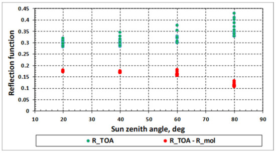
Figure 1.
and the difference under different observation conditions: solar zenith angles from 20 to 80 degrees, viewing angles 0, 15 and 30 degrees, azimuths of observation 45, 90, 135 and 180 degrees. Earth’s surface is sand.
Optically thick clouds are separated from snow pixels with the Normalized Difference Snow Index (NDSI) [11]:
It follows for the snow-covered surfaces: [11].
The detection and discrimination of high cirrus clouds is performed using the condition in the spectral range 1360–1380 nm, where there is a powerful absorption band of water vapor [11]. Therefore, sun light, reflected from the Earth’s surface in this spectral range, practically does not reach the satellite instrument.
2.3. Determination of Water Vapor Content in the Atmosphere
Water vapor is one of the most important components of the atmosphere, affecting the signals recorded by the satellite sensor. The content of water vapor in the atmosphere, in contrast to the content of most atmospheric gases, varies significantly in time and space. Therefore, determining the total content of water vapor in the atmosphere column is important for atmospheric correction of satellite data.
The most common method determining the absorbing gases content in the atmosphere is the differential method, when signals in the absorption band and outside the absorption band at a small distance from it are compared. Wherein it is believed that the remaining parameters of the atmosphere and surface within the absorption band and outside it are the same. Naturally, failure to fulfill this condition can lead to the corresponding error. Moreover, this approach is applicable only in the approximation of the filter model, when we can assume that all absorption takes place at the upper boundary of the atmosphere.
The authors of [12,13,14], consider the Weighting Function Modified Differential Absorption Spectroscopy (WFM-DOAS) technique, where the water vapor content is retrieved only by using the absorption band. However, wherein the proposed models of the atmosphere, underlying surface, and survey geometry are used, the water vapor content is determined in an iterative process based on the ratio:
where W is the total content of water vapor in the atmosphere, is the spectral radiance (SR) measured at the TOA, is the SR, computed for given atmosphere model. The derivative in Equation (3) is calculated at the point . Note that this method is not limited to the applicability of the filter model. However, since its result is the value of W at , it is sensitive to inaccuracies of used atmosphere model, value of surface reflectance and radiometric calibration.
In our opinion, it is preferable to use a slightly different scheme to determine the water vapor content, namely, the iterative process based on the logarithm of the ratio of reflectance values:
Namely, we use iterations as shown below:
where and are SR at the TOA within the absorption band and outside it correspondingly. In this case, the iterative process for retrieving the water vapor content in the atmosphere is arranged according to the scheme:
The function is calculated from the values of measured SR, and value ‘ is determined for the used atmosphere model. In this scheme, as in the WFM-DOAS method, the conditions necessary for the application of filter models and functions, calculated taking into account the atmospheric models and the reflectance of the underlying surface, are not required.
Let us emphasize that since in this scheme the function is defined as the logarithm of the ratio of signals in close spectral ranges, it should be more stable to all errors listed above than in the WFM-DOAS method.
To determine the content of water vapor W in the atmosphere, one can use absorption bands of about 910 nm, 940 nm, or other channels in the range of 900–970 nm with a reference signal in the range of 860–880 nm. The surface spherical reflectance at the wavelength of the reference signal, for example , with a known model of the atmosphere, is easily determined based on the atmospheric correction Equation (9) (see below). To estimate the value of within the absorption band, one can use linear extrapolation over wavelengths of 778.5 nm and 865 nm to the region of the absorption band of water vapor.
Results of computer simulation showed the stability and rapid convergence of scheme (8). Moreover, the simulations demonstrate possibility to retrieve the water vapor content even in cases when parameters of the atmosphere and surface within the absorption band and in the reference channel do not coincide on condition that they are known with good accuracy.
2.4. Aerosol Optical Thickness Retrieval
Most of the known methods and corresponding atmospheric correction algorithms have been designed to determine characteristics of aerosol over dark areas of the Earth’s surface such as vegetation. These surfaces have two characteristic features. The first feature is low reflectance values in the shortwave region. In particular, in the wavelength region about surface reflectance values of the order of 0.01 − 0.04 are characteristic for different types of vegetation (Figure 2). The second feature, in fact, is a consequence of the first one. With such a reflectance, the modulus of the derivative drsurf/dτaer, which determines the error of surface reflectance retrieval depending on the error in the AOT, is quite significant, namely (Figure 3). This means that an error leads to an error in determining the AOT of the atmosphere. This seems to be the main reason for the successful determination of the atmospheric AOT over dark surfaces from multispectral data. Conversely, an error in determining the AOT of the atmosphere leads to an error in surface reflectance retrieving. When moving into the long-wave region, where the surface reflectance usually increases, the error value is noticeably smaller. In the wavelength interval where the derivative is close to zero, even a small error in estimating the surface reflectance leads to a large error in determining the atmospheric AOT. Such a strong sensitivity of the error to the magnitude is due to the fact that in this region the surface reflectance (of the order of ) is close to the reflectance of the aerosol layer of semi-infinite thickness. Therefore, even a significant change in the atmospheric AOT weakly changes the total reflectance of the atmosphere + underlying surface system.
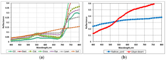
Figure 2.
Spectral reflectance of certain types of vegetation (a) and of sand and desert (b).
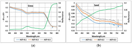
Figure 3.
Reflectance spectra (green line) and derivative for grass (a) and sand (b) at various values of AOT.
Bright surfaces (deserts, various sands) have an reflectance of the order of in the vicinity of (Figure 2). The modulus of derivative is very small, of the order (Figure 3). Therefore, even small errors in the estimation of the surface reflectance can lead to large errors in determining the aerosol optical thickness of the atmosphere. This circumstance makes to be very problematic successful retrieval atmospheric AOT over bright surfaces in algorithms based on the processing only spectral data. However, this same circumstance makes it possible to retrieve the spectral reflectance of the earth’s surface with satisfactory accuracy, since the error of the reflectance retrieval is weakly sensitive to the error of the atmospheric AOT. Indeed, in the case of a bright Earth’s surfaces, even an error should lead to an error of the order of 0.01 − 0.02 in the retrieved surface reflectance in the short-wave region of the spectrum.
From the above, three important conclusions follow that determine the main feature of the RACE algorithm:
- (1)
- The minimum sensitivity of error to error occurs for dark surfaces in the short wavelength region of the spectrum. Therefore, it is optimal to determine the AOT above dark surfaces in the short wavelength region of the spectrum.
- (2)
- The sensitivity of error of retrieved reflectance of dark surfaces to AOT error is at maximum in the short-wave region of the spectrum. When the surface reflectance increases with the wavelength, the retrieving error decreases even if the AOT of the atmosphere is determined with the same error.
- (3)
- For bright surfaces, the sensitivity of surface reflectance errors retrieving to the errors is significantly less in almost the entire spectral range.
The above conclusions and the narrow range of dark surfaces reflectance variations in the short-wavelength region of the spectrum, noted above, allow us to propose the following:
- to retrieve the AOT from the SR recorded by a satellite sensor at one wavelength in this region, in particular, at a wavelength of 412 nm.
- the surface reflectance (in the absence of additional information) can be taken to be fixed and, for example, equal to the average value for a sample of dark surfaces in Figure 2.
In what follows the atmospheric AOT retrieval with use of these estimations is called single-wavelength retrieval.
We note one more argument in favor of using the shortest wavelength for the retrieval of the atmospheric AOT. Just in this spectral interval, the atmosphere aerosol manifests itself most strongly since it is here where the atmospheric AOT is greatest, and the surface reflectance is minimal.
The single-wavelength method for determining the AOT has some significant advantages in problems of atmospheric correction. The ability to determine the atmospheric AOT without reference to a specific type of underlying surface spectrum makes it possible to use this method even in cases with different types of underlying surfaces, including a water surface, inhomogeneous surfaces (for example, a city), with a mixture of different types of surfaces, etc. Finally, the undoubted advantage of this method is its efficiency, since it does not require complex iterative procedures with large expenditures of computer time.
Moreover, the use of additional wavelengths in some cases can even reduce the accuracy of determining the atmospheric AOT due to the smallness of the derivative and, accordingly, increasing values with growth of the surface reflectance in the long-wavelength region of the spectrum.
It should be noted that if the real surface reflectance at the minimum wavelength noticeably exceeds the selected fixed value, then the retrieved atmospheric AOT value could noticeably exceed its true value. This situation can occur, in particular, in the case of a bright underlying surface.
Unfortunately, when the single-wavelength retrieval algorithm is operating in an automatic mode, it is impossible to determine the true cause of the retrieved high AOT value in the shortwave region, namely, whether it is due to strong atmosphere turbidity or is associated with a high surface reflectance. Therefore, it is proposed to introduce the maximum permissible value of the AOT equal to 0.5 at the wavelength . This means that if for the adopted aerosol model the retrieved AOT value at a wavelength of 550 nm exceeds 0.5, it should be taken equal to 0.5.
The rationale for such a choice of the permissible AOT value is the analysis of the real AOT values of the atmosphere in different regions of the Earth according to MODIS measurements [15]. In most regions of the world, AOT at the wavelength does not exceed 0.5. At the same time, the average AOT(550 nm) over 15,894 measurements around the world is 0.2 [15].
If the real reflectance of the surface at the wavelength of 412 nm is noticeably less than 0.028, then the opposite situation may take place. The value of the AOT retrieved may turn out to be noticeably less than the true value and even less than zero. In this regard, a second artificial limitation is introduced. If the retrieved AOT value at the wavelength of 550 nm turns out to be less than 0.05, then its value is set equal to 0.05. The rationale for this limitation is the fact that, firstly, the actual atmospheric AOT less than 0.05 is very rare, and, secondly, this value corresponds to the minimum root-mean-square error at a wavelength of 550 nm in the BAR algorithm for processing MODIS data [1].
3. Retrieval of the Spectral Reflectance of the Underlying Surface
If a pixel size of the image is large compared to the variance of point spread function (PSF) in the atmosphere, or the averaging is performed over a large area (compared to those of the PSF variance), then the average surface reflectance is defined from the following well-known equation for atmospheric correction [6]:
where is the TOA reflectance of the whole atmosphere above a black underlying surface, and are surface reflectance and TOA reflectance, averaged over the area larger than PSF of the atmosphere, is the total (direct+diffuse) transmittance of the whole atmosphere, is the spherical reflectance of the atmosphere at illumination of atmosphere bottom upwards. We emphasize that in Equation (9) and further the spectral reflectance of the underlying surface is considered to be Lambertian.
For high spatial resolution sensors, the basic equation for atmospheric correction can be written as:
or:
where:
Here is the TOA reflectance when observing a certain pixel “p”, and are direct and diffuse components of the atmospheric transmittance, respectively, is the reflectance of the pixel “p”.
Equation (10) is derived under assumptions that the Earth’s surface reflects incident light according to Lambert’s law, the area of “p” pixel is much smaller than the PSF in the atmosphere and the contribution of the scattered light to the TOA reflectance is the same for all pixels over which averaging is performed.
It follows from Equation (11):
where:
The spectral widths of the high spatial resolution channels in the MZ systems could be quite large (say, 10–30 nm) to provide the high enough values of the signal-to-noise ratio. Therefore, one must account for the spectral behavior of optical properties of atmosphere and underlying surface in the MZ channels during the solution of the inverse problem related to the underlying spectral surface reflectance determination.
Let us integrate Equation (11) with respect to the wavelength with weight . Then it follows:
where:
is the spectral radiance at the TOA in the pixel “p”:
the spectral radiance in the n-th channel, averaged over the area larger than the PSF of the atmosphere, d is the distance from the Earth to the Sun in the astronomical units, is the solar light irradiance at the TOA at , is the spectral sensitivity of the n-th channel with the normalization condition:
It follows from Equation (16) that one cannot determine the real reflectance of the test pixel “p” using the MZ satellite data. However, one can derive the so-called effective reflectance averaged with respect to the wavelength taking into account the width of the n-th channel as specified below:
One can see that the effective reflectance depends on the spectral sensitivity of the receiver .
Based on Equation (15), it can be shown that the effective reflectance of the pixel “p” is related to the spectral radiance in this channel by a linear coupling:
where:
Thus, to restore the spectral reflectance of the underlying surface in the pixels of the MZ system of a high spatial resolution, it is necessary to calculate four transfer functions of the atmosphere, namely , , and .
As seen from relations (24)–(27), with the chosen model of the molecular-aerosol atmosphere, these transfer functions depend on the AOT and content of water vapor in the atmosphere. It is emphasized, that the calculation of these functions is the most laborious. Therefore, the number of such calculations is desirable to minimize. Given that the horizontal scale of changes in the water vapor content in the atmosphere, as a rule, is tens of kilometers, the concentration of water vapor in the atmosphere can be considered the same throughout the frame. In this case, the only atmospheric parameter changing within the image frame is the AOT of the atmosphere.
Therefore, it seems appropriate to calculate once the functions , , and for a certain set of AOT values, form them into a Look-up tables, and subsequently, after retrieving the AOT for the local image area, to retrieve the spectral reflectance of the underlying surface in pixels for the corresponding case based on these Look-up tables using interpolation.
The described procedure was deployed for retrieving spectral reflectance of underlying surfaces in the MZ channels in cases presented in Section 4.
4. Testing the RACE Algorithm
4.1. Testing Method
As noted above, in the process of atmospheric correction of multispectral satellite data when retrieving the spectral characteristics of the underlying surface, unknown optical parameters of the atmosphere, and, in particular, atmospheric AOT, must be determined from the same spectral measurements. It is clear that such a task cannot be solved without some a priori assumptions. Therefore, the purposes of performed testing, which description and results are given below, were:
- to verify the correctness of a priori assumptions used in the RACE algorithm,
- to evaluate the stability and speed of the algorithm,
- to estimate the accuracy of retrieving atmosphere parameters and reflectance of the underlying surface with a fairly wide variation of satellite imagery conditions.
The main test results were obtained using computer simulation of signals recorded by a satellite sensor. The software for simulating these signals was developed and carefully tested. The radiative transfer in the system atmosphere—underlying surface has been simulated with the reliable and accurate code RAY [9]. Besides testing based on available experimental data was carried out. When analyzing the RACE algorithm, four main possible sources of error in retrieving the atmospheric optical parameters and the spectral reflectance of the underlying surface can be identified:
- -
- error of the single-wavelength method to retrieve AOT due to the difference between the real (unknown in practice) surface reflectance and its fixed value at wavelength of 412 nm used in the RACE algorithm;
- -
- error of radiometric calibration of sensors in the MS channels;
- -
- error of radiometric calibration of sensors in the MZ channels;
- -
- mismatch between the a priori model of atmospheric aerosol used and the “real” atmospheric aerosol.
For testing, a basic set of parameters of the atmosphere, underlying surface, and observation geometry was selected the most typical for satellite imagery of the Earth’s surface. This set includes:
- -
- three values of aerosol optical thickness of troposphere equal to 0.1, 0.3 and 0.5 at the wavelength of 550 nm;
- -
- 12 types of underlying surface, seven of which relate to dark surfaces such as vegetation (green vegetation (GV), oat, grass, rye, beet, lawn, soil), and five surfaces are bright (desert, sand, loam, dry and wet concrete);
- -
- two values of the solar zenith angle: 20° and 60°;
- -
- viewing zenith angle 0°;
- -
- atmospheric water vapor column .
For testing, a fixed model of the molecular-gas atmosphere “MidlatitudeSummer” [16], typical for the middle latitudes of the globe, was chosen. The widely used model “Continental” [17], consisting of three fractions with lognormal distributions of particle sizes (29% Water Soluble, 70% Dust, and 1% Soot), was taken as a model of aerosol in the lower troposphere layer. To determine the water vapor content, we used the spectral channels 910–920 nm (absorption band of water vapor) and 865–875 nm (reference channel outside the absorption band). The reflectance of the underlying surface was retrieved in the narrow spectral channels of the MS at wavelengths of 412 nm, 442 nm, 489 nm, 509 nm, 559 nm, 619 nm, 664 nm, 776 nm and 867 nm, and in the MZ spectral channels. The spectral ranges for various MZ channels, the effective wavelengths in them and the parameters of the a priori atmospheric model used for testing are given in Table 1. Table 2 and Table 3 present ranges of reflectance variation of dark and bright surfaces in the MS and MZ spectral channels.

Table 1.
Characteristics of MZ channels and the molecular and aerosol optical thicknesses of the a priori atmosphere model used in testing.
Table 2.
Reflectance ranges of dark and bright surfaces in the MS spectral channels.
Table 3.
The reflectance ranges of dark and bright surfaces in the MZ spectral channels.
To clarify the role of the main sources of errors of the RACE, algorithm testing was carried out both for the base case, when the a priori models used fully corresponded to the "real" conditions, and for the cases when the models used and the "real" conditions do not coincide. The influence of all four sources of errors noted above was considered. We emphasize that in all cases the retrieval of parameters of the atmosphere and surface was carried out with the same a priori assumptions. For retrieving AOT, the used earth’s surface reflectance at 412 nm was 0.028. The test results are presented in Figure 4, Figure 5, Figure 6, Figure 7, Figure 8 and Figure 9, in Table 4, Table 5, Table 6, Table 7, Table 8, Table 9, Table 10, Table 11, Table 12 and Table 13 and discussed in what follows.
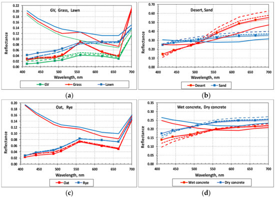
Figure 4.
Reflectance of dark surfaces ((a) and (c)) and bright surfaces ((b) and (d)): true (solid lines with badges) and retrieved with three values of AOT (0.1-short strokes, 0.3-long strokes and 0.5-dash-dot), as well as the SRs at the top-of-atmosphere at AOT 0.03 (solid lines without icons).
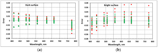
Figure 5.
Errors in retrieving surface spectral reflectance in the MS channels for dark surfaces (a) and bright surfaces (b) at solar zenith angles 60° (red circles) and 20° (green triangles).
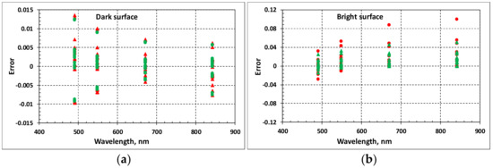
Figure 6.
Errors in retrieving surface spectral reflectance in the MZ channels for dark surfaces (a) and bright surfaces (b) at solar zenith angles 60° (red circles) and 20° (green triangles).
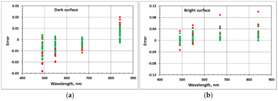
Figure 7.
Errors in retrieving surface spectral reflectance in the MZ channels for dark surfaces (a) and bright surfaces (b) at solar zenith angles 60° (red circles) and 20° (green triangles). Radiometric calibration error in the MS channel 412 nm is 5%.
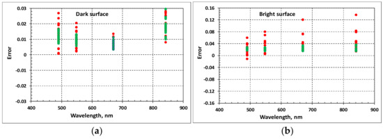
Figure 8.
Errors in retrieving surface spectral reflectance in the MZ channels for dark surfaces (a) and bright surfaces (b) at Sun zenith angles 60° (red circles) and 20° (green triangles), an error of radiometric calibration in the MZ HR channels being 5%.
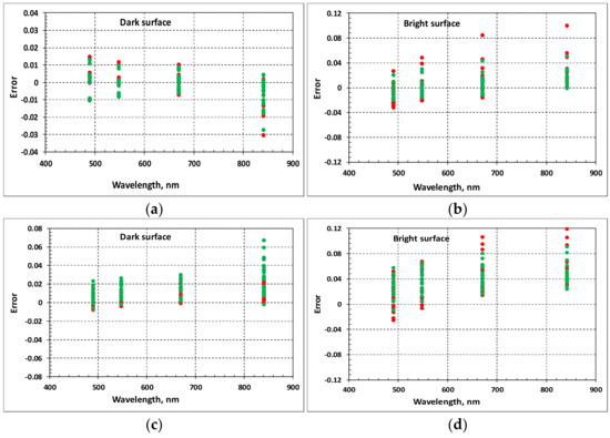
Figure 9.
Errors in retrieving spectral reflectance of dark surfaces (a,c) and bright surfaces (b,d) in the MZ channels in the cases with “Belarus” (a,b) and ”Oceanic” (c,d) models as a true “real” atmospheric aerosol. Zenith angles of the solar are 60° (red circles) and 20° (green circles).
Table 4.
Values of AOT at , retrieved for models of various underlying surfaces under the assumption , and RMSE, with three values of the real and solar zenith angles 60° (upper numbers) and 20° (lower numbers).
Table 5.
RMSE of reflectance retrieval in the MS spectral channels for dark (upper numbers) and bright (lower numbers) surfaces.
Table 6.
RMSE of reflectance retrieval for dark (upper numbers) and bright (lower numbers) surfaces in the MZS HR channels.
Table 7.
RMSE of reflectance retrieval for dark surfaces (upper numbers) and bright surfaces (lower numbers) in the MZ spectral bands with an error 5% of radiometric calibration in the MS channel 412 nm.
Table 8.
RMSE of reflectance retrieval for dark surfaces (upper numbers) and bright surfaces (lower numbers) in the MZ spectral channels with an error 5% of radiometric calibration in these channels.
Table 9.
Optical and microphysical parameters of aerosol models.
Table 10.
RMSE of AOT retrieval with various models of underlying dark surfaces in cases with aerosol models “Belarus” and “Oceanic” considered as true «real» atmospheric aerosols.
Table 11.
RMSE of reflectance retrieval for dark surfaces (upper numbers) and bright surfaces (lower numbers) in the MZ spectral channels in the cases of “Belarus” and “Oceanic” models as a “real” atmospheric aerosol.
Table 12.
Resulting RMSE of surface reflectance retrieval in the MZ channels and the contribution of various sources of error. Case with a dark underlying surface.
Table 13.
Resulting RMSE of surface reflectance retrieval in the MZ channels and the contribution of various sources of error. Case with a bright underlying surface.
4.2. The Influence of the Error of the Atmospheric AOT Retrieval with The Single-Wavelength Method
First, let us estimate the errors in retrieving the parameters of the atmosphere and the reflectance of the underlying surface in the basic version, when the a priori models used fully correspond to the “real” conditions. Thereby, we estimate the error in the determination of the atmospheric AOT due to the difference between the real (unknown in practice) reflectance of the surface and its fixed value at a wavelength of 412 nm used in the RACE single-wavelength algorithm.
Table 4 presents the results of retrieval AOT at for a few underlying surface models and the root mean square errors (RMSE) for three values of the real AOT and solar zenith angles 60° and 20°. For comparison, the last column of Table 4 shows the results of estimation the RMSE at a wavelength of 550 nm in the BAR algorithm for processing MODIS data [1].
Note that in the cases of a high surface reflectance at the wavelength 412 nm, retrieved AOT values almost in all cases turned out to be 0.5. Therefore, we do not present the results of a similar test for the case of bright surfaces.
Figure 4 and Figure 5 illustrate the accuracy of retrieving reflectance of dark and bright underlying surfaces when determining the AOT by the proposed method. One can see that for dark surfaces the error weakly depends on the solar zenith angle and does not exceed 0.02. The maximum error occurs at the shortest wavelength of 412 nm and decreases with increasing wavelength. For bright surfaces, for which the surface reflectance is significantly higher, the reflectance retrieval error is also greater, especially at the solar zenith angle 60°. It is obvious that in this case the error in retrieval AOT manifests itself more pronounced. The errors of the surface reflectance retrieval calculated in the MS spectral channels from these data are presented in Table 5. Note that RMSE do not exceed 0.01 in the case of dark surfaces and 0.025 in the case of bright surfaces.
Errors of the spectral reflectance retrieval in the MZ channels are presented in Figure 6. Naturally, in this case as well, the maximum error of surface reflectance retrieval for dark surfaces occurs in the short-wave MZ channel, wherein it does not exceed 0.015. Table 6 presents RMSE for the surfaces’ reflectance retrieval computed with these data. These errors are less than 0.01 for dark surfaces, about 0.02–0.03 for bright surfaces at the solar zenith angle of 60°, and about 0.01–0.02 at the solar zenith angle of 20°.
4.3. Influence of Errors of Sensors Radiometric Calibration in the MS and MZ Spectral Channels
Errors in radiometric calibration of sensors in the MS spectral channels affect the results of atmospheric correction in two ways. First, the calibration error at a wavelength of 412 nm leads to errors in the determination of the atmospheric AOT and, as a consequence, to errors in the retrieval of the surface reflectance both in the MS and the MZ channels. In addition, calibration errors in the MS spectral channels affect the accuracy of the retrieval of the water vapor content in the atmosphere. The errors in the sensor calibration in the MZ spectral channels directly affect the accuracy of retrieving the surface reflectance in these channels. Below, when analyzing the test results, the calibration error of the MS and MZ sensors in all spectral channels is supposed to be the same and equal to 5%.
Figure 7 clearly shows that overestimation of the MS calibration at a wavelength of 412 nm and, as a result, overestimation of retrieved AOT value, leads, as one would expect, to underestimation of the retrieved values of the spectral surface reflectance in the MZ channels for dark surfaces and to overestimation for bright surfaces. Table 7 displays the RMSE in retrieved values of surface reflectance in the MZ channels.
4.4. The Effect of Discrepancy between the Used a Priori and “Real” Models of Atmospheric Aerosol
One of the main sources of possible errors in the RACE algorithm products is the mismatch between the used a priori and the “real” models of atmospheric aerosols. The fact is that atmospheric correction of MS satellite data does not allow to determine parameters of “real” atmospheric aerosols. Therefore, in the automatic express version of atmospheric correction proposed here, it is necessary to use a fixed, a priori selected aerosol model, for which we recommend using the described above model with aerosol “Continental” for lower and middle tropospheric layers. In this regard, the question of the error caused by the mismatch between the a priori model of aerosol used and the “real” atmospheric aerosol in the case seems to be non-trivial and especially important.
In a presented computer test, we examined atmospheric correction with three different models of “real” aerosol in the lower tropospheric layer, namely “Belarus”, “Maritime” and “Oceanic” [17]. The signals recorded by satellite sensors at TOA in these cases were simulated with the RAY code [9]. Let us underline that in all cases, the retrieval of the atmosphere parameters and reflectance of underlying surfaces was carried out with the a priori selected aerosol model “Continental”.
Let us explain this choice of “real” aerosol models.
The “Belarus” model is based on statistical data on the microphysical parameters of atmospheric aerosol for the spring-summer-autumn period for the territories of the Republic of Belarus and Poland. It contains relatively small particles. The “Maritime” and “Oceanic” models, on the contrary, contain large watered salt particles and describe the scattering of light in the troposphere over oceans. Thus, these selected models include two extreme cases, and the a priori model “Continental” corresponds to intermediate situations. Table 9 lists some important optical and microphysical parameters of these aerosol models, namely, the effective particle size of the aerosol particles , single scattering albedo (SSA), the phase function value at an angle of 120°, , and the Angstrom parameter determining the spectral dependence of the atmospheric AOT, .
An analysis of the test results showed that the errors in spectral reflectance retrieving in cases of “real” “Maritime” and “Oceanic” aerosol models are approximately the same. Therefore, below we restrict ourselves to reviewing the test results only for the “Belarus” and “Oceanic” models. Table 10 presents the RMSE of the AOT retrieval for different models of the dark underlying surface. The RMSE in retrieving spectral reflectance of underlying surfaces in the MZ channels for cases when “Belarus” and “Oceanic” aerosol models are used as “real” atmospheric aerosols are displayed in Figure 9 and Table 11.
It can be seen from Table 10 that the use of the “Continental” aerosol model instead of “real” aerosol models “Belarus” and “Oceanic” in the atmospheric correction procedure can lead to significant errors in the retrieved values of AOT at a wavelength of 550 nm. Added to this is the difference in the spectral behavior of “real” and retrieved AOT values. However, it is a matter of fact that the comparison of Table 11 and Table 6 shows that this discrepancy does not lead to a significant increase in the error of retrieved value of reflectance of the underlying surface (especially in the cases with dark surfaces), even despite the fundamentally different AOT spectral behavior of the “Continental” and “Oceanic” models.
4.5. Resulting Errors in Retrieval of the Underlying Surface Reflectance in the MZ Channels. The Contribution of Various Factors
Let us assume that the contributions of various sources of error to the resulting error in retrieved value of the surface reflectance are independent. In this case, the RMSE can be calculated by the formula:
where are the RMSE of the main sources of error.
Table 12 and Table 13 present resulting RMSE in retrieved surface reflectance in the MZ channels and the contribution from various sources of errors. Note, that the error averaged over models “Belarus” and “Oceanic” was accepted as an error due to mismatch between the a priori model of atmospheric aerosol used and the “real” atmospheric aerosol. It can be seen that the resulting error of the spectral reflectance retrieval in the MZ channels is approximately 0.01–0.02 in the case of a dark surface, while in the case of a bright surface it is of the order of 0.03–0.04. Moreover, in the case of a dark underlying surface, just inaccuracies of radiometric calibration made the main contribution to the resulting error, while in the case of a bright surfaces, errors of single-wavelength method, of the MZ sensors calibration, and of atmospheric model are about the same order. The final rows in Table 12 and Table 13 display the resulting errors in the absence of a calibration error in the MZ channels. As seen, in this case, the error in the retrieving reflectance of dark surfaces becomes noticeably smaller, and that of bright surfaces changes slightly.
Table 14 presents a comparison of the accuracy of the RACE algorithm according to the data of Table 12 and Table 13 with the accuracy of the known algorithms Fast Line-of-sight Atmospheric Analysis of Spectral Hypercubes (FLAASH) [18] of the ENVI package and Digital Globe Atmospheric Compensation (DG AComp) [4] according to [19].
Table 14.
Comparison of the accuracy of surface reflectance retrieval by different algorithms.
It should be emphasized that the test results of the RACE algorithm presented in the paper were obtained for the case of the algorithm operating in a (blind) automatic mode. It can be expected that when operating in operator mode, when it is possible to use information about the type of underlying surface and the type of aerosol in the survey area, the accuracy of determining the surface reflectance may be higher. This primarily applies to areas with a bright surface, where the reflectance at a wavelength of 412 nm is much higher than the a priori accepted .
4.6. Testing the RACE Algorithm Using Experimentally Measured Ground Reflectance Data
Testing was carried out using measurement data on three test sites ((La Crau, France; Railroad Valley, NV, USA; Gobabeb, Namibia) with three different types of underlying surfaces, obtained by the Radiometric Calibration Network (RadCalNet) [20]. In all three cases, ground-based measurements provided spectral surface reflectance, temperature and atmospheric pressure, ozone and water vapor content in the atmosphere, and AOT at the wavelength of 550 nm. In addition, the surface height above sea level and the observation geometry are known [20]. Table 15 presents some of the most important data on the test sites and experimental conditions.
Table 15.
Data on test sites and experimental conditions used for testing the RACE algorithm.
The surface reflectance data were converted to top-of-atmosphere reflectance within RadCalNet and provided through a web portal to allow users to either radiometrically calibrate or verify the calibration of their sensors of interest. These converted data were used for testing the RACE algorithm operating in automatic mode. This means that in all three cases retrieving atmosphere parameters and reflectance of underlying surfaces was carried out with the same a priori basic atmospheric model described above (latitudinal model of the molecular atmosphere, three-layer model of the aerosol atmosphere with aerosol “Continental” in the lower and middle tropospheric layers). Beside while determining the atmospheric AOT, the underlying surface reflectance at the wavelength of 412 nm was assumed equal to 0.028. Additionally, real data on the surface height and observation geometry, as well as on the content of ozone and water vapor were used.
The results of retrieving the spectral reflectance of the surface by the RACE algorithm in comparison with the data of real ground measurements are presented in Figure 10 and in Table 16. Besides, the Table 16 displays the measured and retrieved atmospheric AOT values and errors of surface reflectance retrieval calculated as the difference between the retrieved and measured values. It can be seen that despite considerable errors in retrieving AOT over bright surfaces (Railroad Valley, NV, USA and Gobabeb, Namibia) the surface reflectance is retrieved in all cases with acceptable accuracy.
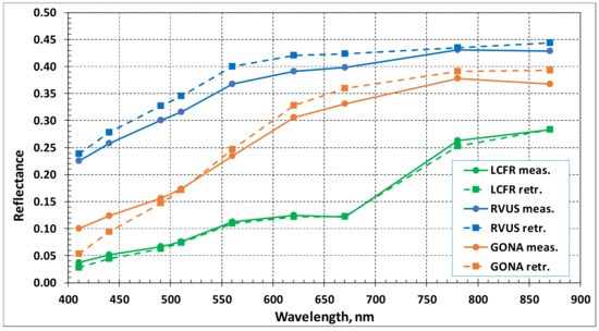
Figure 10.
Spectral reflectance of the surface at test sites La Crau, France (LCFR), Railroad Valley, NV, USA (RVUS), and Gobabeb, Namibia (GONA) according to ground measurements (solid lines) and data retrieved with RACE algorithm (dashed lines).
Table 16.
The results of retrieving spectral reflectance of surfaces with the RACE algorithm in comparison with the data of reflectance ground measurements.
As for significant errors in retrieving values of small AOTs over bright surfaces, let us note that this feature is characteristic for all existing algorithms. Physical reasons have been described above. However, it may be worth recalling that the AOT retrieval is not the objective point for the RACE algorithm, aimed at the effective retrieval of a surface spectral reflectance in an automatic mode in situations with lack of information about underlying surface.
5. Conclusions
In this paper we have presented a simple and robust technique for retrieving surface spectral reflectance using spectral reflectance measurements captured by satellite instruments with high or moderate spatial resolution and with limited amount of available auxiliary information.
The key point of this algorithm is the suggested single-wavelength method for estimating the atmospheric AOT at 400 nm. This method is mainly based on two factors.
First, low spectral ground reflectance values and its low variability (of the order of 0.01 − 0.04) in vicinity are characteristic for a wide class of dark areas (vegetation types) of the Earth’s surface.
With such surface reflectance values, the dependence of the error in the AOT estimation on the error in specifying the surface reflectance has a minimum.
Second, although for bright surfaces, such as deserts and semi-deserts, errors in AOT retrieval may be noticeably greater than in the previous case, the sensitivity of surface reflectance errors to the errors is significantly smaller in almost entire spectral range.
Other important classes of objects are seas and oceans. Considering that the reflectance of water basins in the region is approximately the same as that of vegetation, the proposed technique is promising for satellite monitoring of water basins as well.
The retrievals, performed with computer simulations and use of experimental data, have demonstrated a sufficient retrieval accuracy.
Thus, the proposed technique can be used to retrieve the reflectance of various underlying surfaces in an automatic mode without huge databases accumulated in advance.
Author Contributions
Conceptualization, I.L.K. and A.S.P.; methodology, I.L.K. and E.P.Z., software, A.S.P.; validation, I.L.K. and A.S.P.; formal analysis, I.L.K.; investigation, I.L.K., A.S.P.; resources, I.L.K.; data curation, A.S.P.; writing—original draft preparation, I.L.K., A.S.P., E.P.Z. and A.A.K.; writing—review and editing, I.L.K. and E.P.Z.; visualization, A.S.P.; supervision, I.L.K. All authors have read and agreed to the published version of the manuscript.
Funding
This research received no external funding.
Institutional Review Board Statement
Not applicable.
Informed Consent Statement
Not applicable.
Data Availability Statement
Data is available on request.
Acknowledgments
We are grateful to a Radiometric Calibration Network (RadCalNet) for Earth observing imagers operating in the visible to shortwave infrared spectral range.
Conflicts of Interest
The authors declare no conflict of interest.
References
- Lipponen, A.; Mielonen, T.; Pitkänen, M.R.A.; Levy, R.C.; Sawyer, V.R.; Romakkaniemi, S.; Kolehmainen, V.; Arola, A. Bayesian aerosol retrieval algorithm for MODIS AOD retrieval over land. Atmos. Meas. Tech. 2018, 11, 1529–1547. [Google Scholar] [CrossRef]
- Hsu, N.C.; Tsay, S.-C.; King, M.D.; Herman, J.R. Aerosol Properties Over Bright-Reflecting Source Regions. IEEE Trans. Geosci. Remote Sens. 2004, 42, 557–569. [Google Scholar] [CrossRef]
- Hsu, N.C.; Jeong, M.-J.; Bettenhausen, C.; Sayer, A.; A Hansell, R.; Seftor, C.S.; Huang, J.; Tsay, S.-C. Enhanced Deep Blue aerosol retrieval algorithm: The second generation. J. Geophys. Res. Atmos. 2013, 118, 9296–9315. [Google Scholar] [CrossRef]
- Atmospherc Compensation in Satellite Imagery. U.S. Patent 9,396,528 B2, 19 July 2016.
- Kinne, S.; O’Donnel, D.; Stier, P.; Kloster, S.; Zhang, K.; Schmidt, H.; Rast, S.; A Giorgetta, M.; Eck, T.F.; Stevens, B. MAC-v1: A new global aerosol climatology for climate studies. J. Adv. Model. Earth Syst. 2013, 5, 704–740. [Google Scholar] [CrossRef]
- Katsev, I.L.; Prikhach, A.S.; Zege, E.P.; Ivanov, A.P.; Kokhanovsky, A.A. Iterative procedure for retrieval of spectral aerosol optical thickness and surface reflectance from satellite data using fast radiative transfer code and its application to MERIS onboard ENVISAT measurements. In Satellite Aerosol Remote Sensing over Land; Kokhanovsky, A.A., de Leeuw, G., Eds.; Springer: Heidelberg, Germany, 2009; pp. 101–134. [Google Scholar]
- Von Hoyningen-Huene, W.; Freitag, M.; Burrows, J.B. Retrieval of aerosol optical thickness over land surfaces from top-of-atmosphere radiance. J. Geophys. Res. Space Phys. 2003, 108, 4260–4272. [Google Scholar] [CrossRef]
- Katsev, I.L.; Prikhach, A.S.; Zege, E.P.; Grudo, J.O.; A Kokhanovsky, A. Speeding up the aerosol optical thickness retrieval using analytical solutions of radiative transfer theory. Atmos. Meas. Tech. 2010, 3, 1403–1422. [Google Scholar] [CrossRef]
- Tynes, H.; Kattawar, G.W.; Zege, E.P.; Katsev, I.L.; Prikhach, A.S.; Chaikovskaya, L.I. Monte Carlo and multicomponent ap-proximation methods for vector radiative transfer by use of effective Mueller matrix calculations. Appl. Opt. 2001, 40, 400–412. [Google Scholar] [CrossRef] [PubMed]
- Kokhanovsky, A.A. Reflection of light from nonabsorbing semi-infinite cloudy media. A simple approximation. J. Quant. Spectrosc. Radiat. Transf. 2004, 85, 25–33. [Google Scholar] [CrossRef]
- LANDSAT 8 (L8). Data Users Handbook; Version 2.0; EROS: Sioux Falls, SD, USA, 29 March 2016. [Google Scholar]
- Buchwitz, M.; Rozanov, V.V.; Burrows, J.P. A near-infrared optimized DOAS method for the fast global retrieval of atmospheric CH4, CO, CO2, H2O, and N2O total column amounts from SCIAMACHY Envisat-1 nadir radiances. J. Geophys. Res. Space Phys. 2000, 105, 15231–15245. [Google Scholar] [CrossRef]
- Buchwitz, M.; Burrows, J.P. Retrieval of CH 4, CO, and CO 2 total column amounts from SCIAMACHY near-infrared nadir spectra: Retrieval algorithm and first results. In Proceedings of the Remote Sensing of Clouds and the Atmosphere VIII, Barcelona, Spain, 9–12 September 2003; Volume 5235, pp. 375–389. [Google Scholar] [CrossRef]
- Noel, S.; Buchwitz, M.; Burrows, J.P. First retrieval of global water vapour column amounts from SCIAMACHY meas-urements. Atmos. Chem. Phys. 2004, 4, 111–125. [Google Scholar] [CrossRef]
- Gupta, P.; Remer, L.A.; Levy, R.C.; Mattoo, S. Validation of MODIS 3 km land aerosol optical depth from NASA’s EOS Terra and Aqua missions. Atmos. Meas. Tech. 2018, 11, 3145–3159. [Google Scholar] [CrossRef]
- AFGL-TR-86-0110. Atmospheric Constituent Profiles (0–120 km); Environmental Research Papers No. 954 ADA175173; US Air Force Geophysics Laboratory: Hanscom, MA, USA, 1986.
- Lenoble, J. A Preliminary Cloudless Standard Atmosphere for Radiation Computation; World Climate Programme, World Meteorological Organization: Geneva, Switzerland, 1986; Volume 112, pp. 1–40. [Google Scholar]
- Perkins, T.C.; Adlergolden, S.M.; Matthew, M.W.; Berk, A.; Bernstein, L.S.; Lee, J.; Fox, M.J. Speed and accuracy improvements in FLAASH atmospheric correction of hyperspectral imagery. Opt. Eng. 2012, 51, 111707. [Google Scholar] [CrossRef]
- Smith, M.J. A Comparison of DG AComp, FLAASH and QUAC Atmospheric Compensation Algorithms Using WorldView-2 Imagery/University of Colorado. 2015. Available online: https://digitalglobe-marketing.s3.amazonaws.com/files/blog/ (accessed on 24 June 2016).
- Bouvet, M.; Thome, K.; Berthelot, B.; Bialek, A.; Czapla-Myers, J.; Fox, N.P.; Goryl, P.; Henry, P.; Ma, L.; Marcq, S.; et al. RadCalNet: A Radiometric Calibration Network for Earth Observing Imagers Operating in the Visible to Shortwave Infrared Spectral Range. Remote Sens. 2019, 11, 2401. [Google Scholar] [CrossRef]
Publisher’s Note: MDPI stays neutral with regard to jurisdictional claims in published maps and institutional affiliations. |
© 2021 by the authors. Licensee MDPI, Basel, Switzerland. This article is an open access article distributed under the terms and conditions of the Creative Commons Attribution (CC BY) license (https://creativecommons.org/licenses/by/4.0/).