Technical Note

A Robust and Fast Collision-Avoidance Approach for Micro Aerial Vehicles Using a Depth Sensor †

1
Computer Vision and Aerial Robotics Group (CVAR), Centre for Automation and Robotics (CAR), Universidad Politécnica de Madrid (UPM-CSIC), Calle Jose Gutiérrez Abascal 2, 28006 Madrid, Spain
2
Dronomy, Paseo de la Castellana 40, 28046 Madrid, Spain
*
Author to whom correspondence should be addressed.
This paper is an extended version of our paper published in Lu, L.; Sampedro, C.; Rodriguez-Vazquez, J.; Campoy, P. Laser-based collision-avoidance and Reactive Navigation using RRT* and Signed Distance Field for Multirotor UAVs. In Proceedings of the 2019 International Conference on Unmanned Aircraft Systems (ICUAS), Atlanta, GA, USA, 11–14 June 2019.
Remote Sens. 2021, 13(9), 1796; https://doi.org/10.3390/rs13091796
Submission received: 22 March 2021 / Revised: 7 April 2021 / Accepted: 2 May 2021 / Published: 5 May 2021

Abstract

:
Collision-avoidance is a crucial research topic in robotics. Designing a collision-avoidance algorithm is still a challenging and open task, because of the requirements for navigating in unstructured and dynamic environments using limited payload and computing resources on board micro aerial vehicles. This article presents a novel depth-based collision-avoidance method for aerial robots, enabling high-speed flights in dynamic environments. First of all, a depth-based Euclidean distance field mapping algorithm is generated. Then, the proposed Euclidean distance field mapping strategy is integrated with a rapid-exploration random tree to construct a collision-avoidance system. The experimental results show that the proposed collision-avoidance algorithm has a robust performance at high flight speeds in challenging dynamic environments. The experimental results show that the proposed collision-avoidance algorithm can perform faster collision-avoidance maneuvers when compared to the state-of-art algorithms (the average computing time of the collision maneuver is 25.4 ms, while the minimum computing time is 10.4 ms). The average computing time is six times faster than one baseline algorithm. Additionally, fully autonomous flight experiments are also conducted for validating the presented collision-avoidance approach.

1. Introduction

Collision-avoidance using onboard sensing is a key topic in the robotics field. The challenge involves the robot being able to move in a totally unknown and dynamic environment, without colliding and only with a limited field of view.
In order to overcome the aforementioned challenges, a robust and fast obstacle detection and avoidance algorithm that can perform online localization and planning is presented in this article. In our previous work, a laser-based collision-avoidance strategy was proposed [1,2]. In this work, the previous algorithm has been improved so that it only requires a depth camera. This is a better option for an unmanned aerial platform that has limited payload and computing resources. Except for the algorithms of [1,2], the only forward maneuver (OFM) is proposed in this article to enable collision-avoidance with different yaw angles. In the OFM, the robot starts with a yaw angle that heads to the goal. Thorough simulation and real flight experiments are also given to evaluate the proposed collision-avoidance approach.
Several methods have been proposed during the last few decades to address the problem of collision-avoidance. The visual servoing approaches use the feedback information extracted from vision sensors to plan the motion of robots. Penin et al. [3] developed a vision-based controller and planner for aggressive collision-avoidance and tested it in a real environment. However, their path-planning approach required complete knowledge of the environment and robot model.
Optical flow methods rely on the apparent motion of texture in the visual field relative to the body of the robot. Optical flow-based strategies allow robots to operate collision-avoidance by turning away from regions with high optical flow. An optical flow-based approach was proposed by Simon Zingg et al. [4] for the navigation of micro aerial vehicles in indoor corridors. They used a pyramidal lucas-kanade optical flow detector to estimate the optical flow and compensated for the rotational effects using the inertial measurement unit (IMU) data. In the same direction, Cho et al. [5] also presented a vision-based obstacle avoidance strategy for micro aerial vehicles using the optical flow. Their approach could avoid wall-like frontal obstacles, which was a general limitation in optical flow-based methods. Overall optical flow-based methods have shortcomings in the sense that they generate an artificial parallax that will yield low optic flow values for smaller oncoming obstacles.
Artificial potential field (APF) methods [6,7] use gradient descent planning to find the minimum artificial potential energy. They rely on the calculation of the attractive potential to the goal and repulsive potential from the obstacles and find a trajectory that is collision-free. However, the presence of local minima commonly causes problems in these strategies.
Geometry-based approaches use the geometric relationship between the robot and the obstacles to calculate a path for the robot. Lin et al. [8] presented a collision-avoidance approach for unmanned aerial robots, which combined a collision-avoidance algorithm using geometric primitives and an initial collision time selection algorithm based on kinematic considerations, collision likelihood, and navigation constraints.
Velocity obstacle (VO) methods like [9] use a probabilistic velocity obstacle (PVO) to predict the probability of the uncertainty in obstacles’ position, shape, and velocity. However, it cannot guide the robot to the goal or respond to certain emergency conditions. The work presented in [10] used the acceleration velocity obstacle (AVO) to help the robot avoid obstacles in a dynamic environment while being subject to acceleration constraints. VO-based approaches highly rely on the robot’s model and require accurate measurements of the obstacle’s velocity.
Learning-based methods have also been proposed, such as the one presented in [11], which developed a deep reinforcement learning-based collision-avoidance algorithm inspired by the encirclement behavior of dolphins to entrap the fishes. The work presented in [1] uses a deep reinforcement learning approach to build a reactive navigation algorithm by adopting an APF formulation in the reward function. In their experiments, the algorithm provided appropriate reactive navigation behaviors in simulated and real indoor scenarios with static and dynamic obstacles.
Planning based-algorithms will plan a collision-free trajectory based on the information of obstacles extracted from perception sensors. Lopez et al. [12] presented a relaxed-constraint triple integrator planner (R-TIP) for a collision-avoidance strategy with limited field-of-view sensing. Tackling the problem of narrow field-of-view perception, their planner could choose a motion primitive from the past that made the planning algorithm more efficient. Liu et al. [13] proposed a short-range planner to plan and replan a dynamic feasible trajectory and achieve the obstacle avoidance maneuver in real-time. A real-time mapping, re-localization, and planning approach was presented by Burri et al. [14]. This approach can fly the aerial robot fully autonomouslly in unknown environments without knowing any prior knowledge, and has good planning efficiency. Chen et al. [15] presented an online collision-free trajectory planner for micro aerial vehicles’ autonomous flight in clutter environments. They added the constraints of a safe corridor to build a convex optimization problem, and solved it by using the quadratic programming (QP) approach. Their approach has good computing performance. However, this approach needs to be replanned to make sure that the trajectory is inside the safe corridor that is time-consuming. Tordesillas et al. [16] used a local planner and safe back-up trajectory to solve the safety and fast conflict in the UAV motion planning problem. The time allocation was optimized using a mixed integer quadratic program (MIQP) formulation. More recently, Chen et al. [17] presented a computing efficient obstacle avoidance trajectory planner using an heuristic angular search method and minimum acceleration optimization. Ryll et al. [18] also introduced a receding horizon, sampling-based planner to achieve high-speed collision-avoidance maneuver.
There are two main reasons why the proposed work can achieve a shorter computing time than the state-of-art algorithms. (1) The fast Euclidean distance field-mapping approach that can build the Euclidean distance field directly from the depth input. (2) The fast Euclidean distance field-based collision-checking approach that can reduce the points for collision-checking in the path segment.
The proposed work presented in this paper uses a sampling-based strategy enhanced by computing an Euclidean distance field-based collision-checking algorithm for the collision-avoidance of multirotor aerial robots. The principal goal of this article is to develop a collision-avoidance strategy that can help the aerial robot have a fast reaction to suddenly appearing obstacles when flying at high speeds.
The main contributions of the proposed solution are:
(1)
The presented collision-avoidance method only uses a depth sensor for collision-avoidance and does not need any information about the geometry of the obstacles.
(2)
By using the novel Euclidean distance field-mapping and collision-detection approach, the computing time of the collision-avoidance maneuver can be reduced to a range of 10.4 ms and 40.4 ms that is less than the computing time of the state-of-the-art algorithms.
(3)
In the simulation experiments, the proposed collision-avoidance strategy can fly the robot at 2.4 m/s in challenging dynamic environments with an 82% success rate across 100 repetitive tests. The algorithm can also achieve a 95% success rate of 100 repetitive tests in a challenging static environment with a flight speed of 1.96 m/s.
The remainder of the paper is organized as follows. In Section 2, the problem formulation is introduced. The proposed Euclidean distance field mapping and collision-checking algorithm are described in Section 3 and Section 4. Section 5 calculates the algorithm complexity. The experimental results and discussion are shown in Section 6 and Section 7, respectively. Finally, Section 8 concludes the paper and summarizes future research directions.
The definitions of acronyms used in this article are shown in Table 1.

2. Problem Statement

Recently, unmanned aerial vehicle-based remote-sensing technology has been widely used in areas such as object detection and tracking [19], search and rescue [20], and industrial inspection [21]. The presented collision-avoidance approach can help unmanned aerial vehicles perform autonomous remote-sensing tasks without collision. In the proposed method, the laser/depth camera-based sensing technology is also applied when extracting the Euclidean distance field.
This section firstly introduces the dynamic collision-avoidance problem and how to solve it. The description of the obstacle is then explained. Figure 1 shows the aerial robot used for the real flight experiments and Figure 2 shows the Euclidean distance field-mapping algorithm process.
In the dynamic collision-avoidance problem herein proposed, the environment has an initial point and a goal point, and the robot can only observe a limited part of the environment. The environment has several static or/and moving obstacles. The position and shape of the obstacles are totally unknown when the robot starts to move in the environment. The obstacles can suddenly appear in the flight path of the robot. The robot can move freely in the environment. The robot needs to start at an initial point P i n i t and the task is finished when the robot reaches a spherical region of arbitrary size centered on the goal point P g o a l . The localization information can be provided by ground truth or onboard sensors. It is considered as a collision with an obstacle when the distance from the robot to the surface of the obstacle is less than the radius of the robot.
The dynamic collision-avoidance problem can be solved using the following process: (1) Constructing the Euclidean distance field from the sensor input; (2) planning a collision-free trajectory based on the Euclidean distance field; and (3) replanning when new obstacles are detected in the future flying trajectory. In the proposed approach, obstacles are represented by the function D i s t ( x ) , which is used to compute the distance from any point in the environment to the surface of the nearest obstacles. More detailed information about the obstacle representation can be checked in [2].

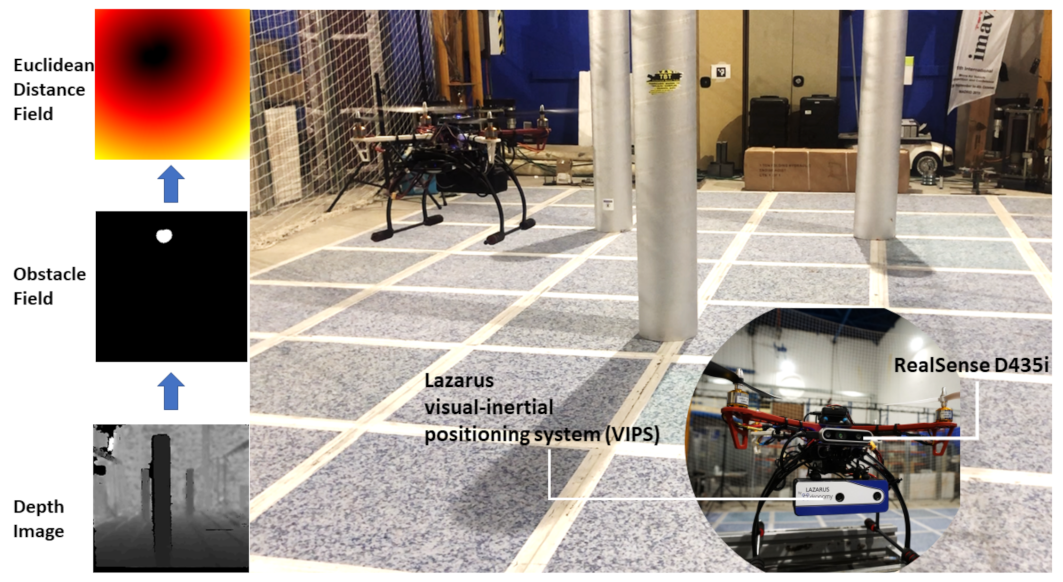
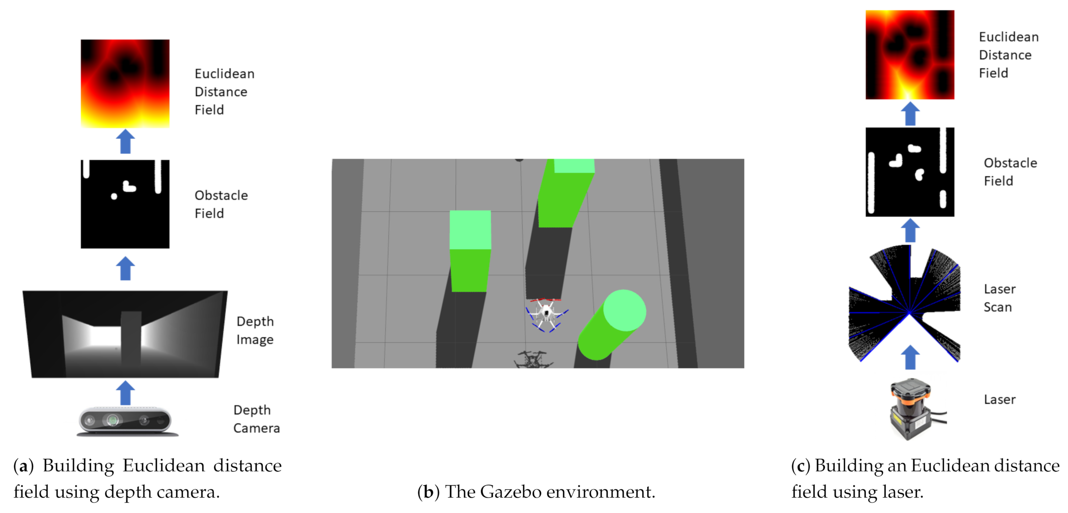
3. Depth-Based Euclidean Distance Field Construction

In this section, firstly, the strategy about how to build the obstacle field from the depth maps of the depth sensor is explained, and then the method for transforming the obstacle field to the Euclidean distance field is presented. As depth cameras and LIDAR sensors are widely used in the area of robot navigation, they are selected as examples to explain how to obtain the Euclidean distance field from the depth map. Figure 2a,c show a diagram with the steps to build an Euclidean distance field from a depth image and from a laser scan, respectively.
Depth sensors can determine the distance from the robot to the objects. By using distance information, the obstacle field can be built.

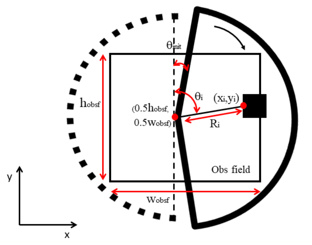
3.1. Building the Obstacle Field Using the Depth Sensor

As can be seen from Figure 2c, laser scan ranges can be obtained from the LIDAR sensor. Based on the laser scan ranges, the position of the point at the end of every laser scan range with respect to the position of the robot can be found. Then, these points are marked as the obstacle region in the obstacle field. The position of the robot is the center of the obstacle field, which represents a collection of the obstacle points. After obtaining the previous obstacle field, the obstacle region is inflated in order to make sure that every obstacle can be presented. The white region of the obstacle field in Figure 2c is the inflated obstacle region. Equation (1) shows the formulations to get the position of obstacle points from laser scan ranges and mark them in the obstacle field, respectively. Figure 3 introduces the obstacle points mapping process of Equation (1):
Δ X i = R i r e s × sin θ i Δ Y i = R i r e s × cos θ i x i = w o b s f 2 + Δ X i y i = h o b s f 2 + Δ Y i θ i = θ i n i t + i × Δ θ i ( 0 , 1 , · · · , R n u m 1 , R n u m ) ,
where r e s is the resolution of the obstacle field. The R i , Δ θ , and R n u m are the length of the range i, the increment of θ in the horizontal field of view and the amount of the ranges of the laser, respectively. The θ i n i t is the initial angle of the ranges of the laser scan, and the θ i is the angle i of the ranges of the laser scan. The Δ X i and Δ Y i are the distances in X and Y axes from the obstacle points ( x i , y i ) to the center of the obstacle field. The w o b s f and h o b s f are the width and height of the obstacle field, respectively.
The strategy of building the obstacle field is similar to the one using the laser. The difference is that the depth image should be transformed into a laser scan first. By transforming the depth image to a laser scan, The ROS package d e p t h i m a g e _ t o _ l a s e r s c a n (http://wiki.ros.org/depthimage_to_laserscan, accessed on 1 March 2021) has been used to transform the depth image to a laser scan.

3.2. Transforming the Obstacle Field to the Euclidean Distance Field

After obtaining the obstacle field, it can be transformed into the Euclidean distance field by the Euclidean distance transform [22]. In order to use the Euclidean distance field for collision-checking, it should be changed from the world frame of reference to the image frame. Equations (2)–(4) provide the formulation for transforming the obstacle field to an Euclidean distance field. Equation (2) shows the Euclidean distance field is constructed based on the obstacle field using Euclidean distance transformation. Equations (3) and (4) shows the transformation of the point in the obstacle field when turning the yaw.
E D F i m g ( x , y , z ) = E D T ( O F ( x , y , z ) )
( x , y , z ) = T 1 × ( X , Y , Z )
T = sin ( ϕ ) cos ( ϕ ) 0 cos ( ϕ ) sin ( ϕ ) 0 0 0 1
In Equations (2)–(4), O F is the obstacle field. The ( x , y, z ) and ( X , Y, Z ) are the coordinates in the image frame and the world frame, respectively. The T is the transformation from the world frame to the image frame. The ϕ is the yaw angle. The EDF means the Euclidean distance field building, while the EDT is the Euclidean distance transformation.

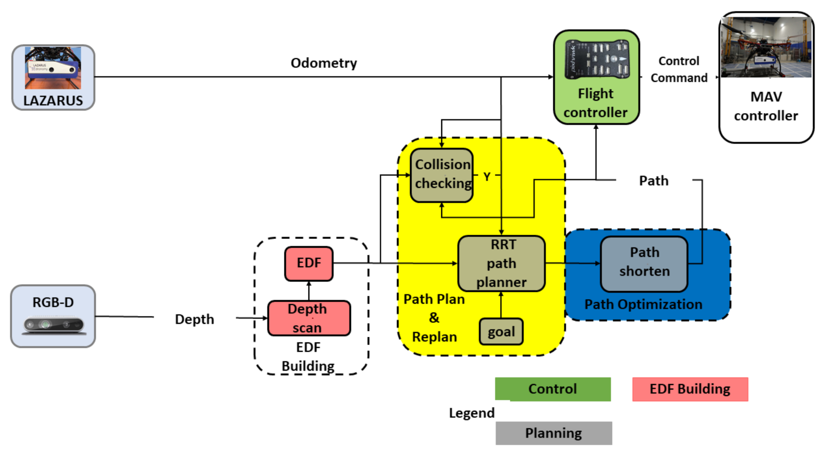
4. Collision-Avoidance Using Euclidean Distance Fields and Rapidly-Exploring Random Tree

In this section, the Euclidean distance field-based collision detection strategy and the rapidly-exploring random tree (RRT)-based collision-avoidance are explained.

4.1. Euclidean Distance Field-Based Collision Detection

The classic collision-checking approach splits the path segment into finite points and then checks the collision status of every point. This method has shortcomings in the sense that the numbers of path points should be manually determined due to different environments, and it is also time-consuming because it checks unnecessary points. By using the Euclidean distance field, these shortcomings can be overcome because using the Euclidean distance field notation, the distance from path points to the nearest obstacle can be directly obtained. Thus, this distance can be used to determine the path points for collision-checking. Equations (5) and (6) show the formulation of the collision-checking algorithm.
x i + 1 = x i + D i s t ( x i ) R r o b o t x i n i t x e n d · x i n i t x e n d
C o l l i s i o n D e t e c t ( x i ) = 1 , D i s t ( x i ) R r o b o t 0 , D i s t ( x i ) > R r o b o t
R r o b o t is the radius of the robot. D i s t ( x i ) is the function to calculate the distance from x i to the nearest obstacle. x i n i t and x e n d are the initial and ending points of the path segment. x i and x i + 1 are the current and next points for collision-checking.

4.2. Collision-Avoidance Planning and Replanning

This section explains how to integrate the proposed collision detecting algorithm with the RRT path planning algorithm to solve the collision-avoidance problem.
The proposed Euclidean distance field-based collision detection algorithm can be used to check the collision of the line segment between the new state and the nearest state of the RRT.
For the path replanning, the Euclidean distance field collision-detecting algorithm is applied for detecting the collision of the path segment between the current robot state and next point in the planned path. In order to save computing resources and avoid changing the flight path, the RRT path-planning algorithm will plan a new path from the current robot state to the goal point only when a future collision is detected.
The planned path is then sent to the polynomial trajectory generation algorithm [23], and the trajectory is then sent to the motion control system [24] to fly the robot.

5. Algorithm Complexity

The algorithm complexity is important when the computing resources of the agent are limited. For every run of the collision-avoidance maneuver, firstly the Euclidean distance field is constructed, then the collision-checking algorithm starts working, and finally, the RRT algorithm is used to search the feasible path.
Euclidean distance field-building: Assuming the obstacle field is an image with the size of w × h, the field of view can be split into k scans. The algorithm complexities of the obstacle field build and the Euclidean distance transform are O ( k ) and O ( 2 × m × n ) , respectively. The complexity of the Euclidean distance field building part is the sum of them that is O ( k ) + O ( 2 × w × h ) .
Collision-checking: Assuming the number of future path points P f and is n. There are m i points required for collision-checking in i-th path segment. The path segment connects the previous P f and current P f . The complexity of the collision-checking part is i = 1 n 1 O ( m i ) .
Path-searching: Assuming the maximum iterations of RRT generation is n u m . In the j-th iteration, there are a j nodes in the rapidly-exploring random tree and b j points needed for collision-checking in the path segment from the nearest node to the new node. The algorithm complexity of the path searching part is j = 1 n u m O ( a j ) + O ( b j ) .
The overall algorithm complexity is the sum of the algorithm complexity that is O ( k ) + O ( 2 × w × h ) + i = 1 n 1 O ( m i ) + j = 1 n u m O ( a j ) + O ( b j ) .

6. Experiments and Results

A video description of the experiments is shown in: https://vimeo.com/474208476, accessed on 01 March 2021.

6.1. Experimental Setup

In this subsection, the experimental setup for the simulation experiments and real flights is introduced.
The simulation experiments are run on top of Ubuntu 18.04 using the Robot Operating System (ROS) [25]. The Gazebo environment is used to provide the environment model, and the RotorS [26] simulation is used to provide the real physical parameters of the robot. All the experiments were run on a laptop with Intel Core i7-8750H at 2.2 GHz. The robot in the simulation is a multirotor robot (AscTec Firefly) that has six degrees of freedom, which was equipped with an RGB-D camera and an odometry sensor. The RGB-D camera captures the information from the outside environment. The localization of the robot was achieved with the odometry sensor. The horizontal and vertical field of view of the RGB-D camera are 114 and 60 . The maximum and minimum range of the RGB-D sensor are 0.15 m and 3 m, respectively. The resolution of the Euclidean distance field is 0.02 m.
The robot can fly in the 3D simulation environment, but the information used to perform obstacle avoidance is 2D.
In order to provide different velocity modes, the closed-form trajectory-generation method [23] is applied for generating trajectory commands within the maximum velocity and acceleration. Finally, the trajectory command is sent to a model predictive controller [24] to move the robot.
The real flight experiments are carried out using an aerial platform. As can be seen from Figure 4, the aerial platform has an intel RealSense D435i depth camera to receive the information from the environment and a Pixhawk module to serve as a flight control unit. For the localization, the robot is equipped with Lazarus, a commercial visual-inertial positioning system (VIPS) manufactured by the Spanish company Dronomy. It relies on two front-looking cameras and a highly-stable, six-axis IMU. The Jetson TX2 with a dual-core NVIDIA Denver 2 64-bit CPU and NVIDIA Pascal TM Architecture GPU is chosen as the on-board computer. The weight of the aerial robot is 1860 g without batteries.
A random shortcut algorithm [27] is used to optimize the path generated by the planning module. All the real flight experiments were executed using on-board perception and localization in a GPS-denied scenario.

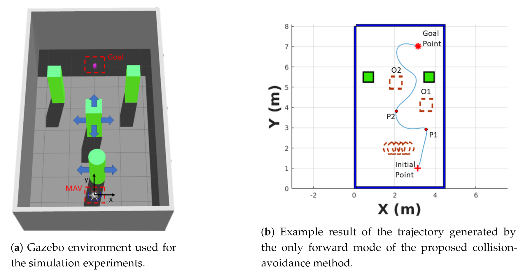
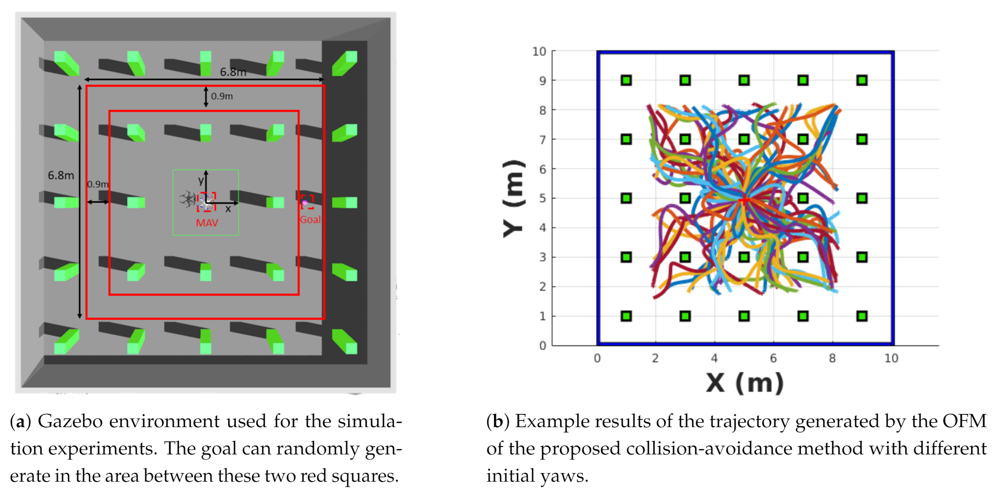
6.2. Simulation Experimental Results

As can be seen from Figure 5a, in order to validate the proposed approach in challenging conditions, a dynamic Gazebo environment of 4.4 × 8 × 1.5 m was created. The Gazebo environment contains four obstacles that have different movements (two static quadrilateral obstacles, a quadrilateral obstacle that can suddenly appear in front of the robot, and a cylindrical obstacle which has a sinusoidal trajectory). In the simulation environment, the x coordinates of the centers of the static quadrilateral obstacles are −1.5 m and 1.5 m, respectively, while their y coordinates are both 5.5 m. The x coordinate position of the moving quadrilateral obstacle can change from (2.6 m, 2.64 m) and (3.7 m, 3.75 m). The moving cylindrical obstacle starts moving from (2 m, 0 m). The initial and goal points are randomly generated for each repetitive experiment. The size of the quadrilateral obstacle is 0.5 × 0.5 × 2 m, while the cylindrical obstacle is a cylinder with a base radius of 0.3 m and a height of 2 m. The random generation range for the initial and goal point are from (1 m, 1 m) to (3 m, 1 m) and (1 m, 7 m) to (3 m, 7 m), respectively. Figure 5b shows a sample result of the trajectory generated by the OFM of the collision-avoidance strategy.
Figure 6a shows the simulation environment used to evaluate the proposed collision with different initial yaw angles. The value of the initial yaw angle is computed as a r c t a n ( y g o a l x g o a l ) . The initial point of this simulation is always (0 m, 0 m, 1.1 m). The goal point can be generated randomly between the two red boxes in Figure 6a. The size of the quadrilateral obstacle is 0.3 × 0.3 × 2 m, and the positions are shown in Figure 6b. The 95 success trails out of 100 trails of the proposed algorithm are shown in Figure 6b.
The objective of the robot is to reach the goal starting at the initial point. In Table 2, the experiments are conducted using four different collision-avoidance algorithms. Two of them are state-of-the-art learning-based strategies, which are the DDPG [1] and NAF [28]. The other two are the only forward maneuvers (OFM) of the presented algorithm. Among them, the only forward maneuver with high velocity (OFM_HIGH), and the only forward maneuver with low velocity (OFM_LOW) mean flying the robot with high velocity (maximum velocity is set as 2.5 m/s) and low velocity (maximum velocity is set as 2 m/s). In Table 3, the maximum velocities for the OFM are 2 m/s. In order to provide representative metrics, 100 runs were conducted for each algorithm in both simulation environments.
The collision-checking time and the trajectory computing time in Table 4 was collected from the 100 trails of the simulation experiments in Figure 6a. In these 100 trials, there are 220 times replan due to the appearance of unknown obstacles. The average collision-checking time and trajectory computing time with their standard deviations of these 100 trials are 9 ± 5 ms and 16.3 ± 10 ms, respectively.

6.3. Real Flight Experimental Results

There are two different cases designed for real flight experiments. One is a one-cylinder case and the other is a three-cylinder case. The start points of these two scenarios are (0, 0, 0), while the endpoints of one cylinder and three cylinders’ environments are (0, 4, 0) and (0, 5, 0), respectively. The maximum velocities in the one cylinder and three cylinders cases are 0.32 m/s and 0.44 m/s. Figure 7a,c show the trajectories of these two experiments, while Figure 7b,d show how the velocities vary during the experiments.
The purpose of the real flight experiments was to confirm that the proposed collision-avoidance algorithm can run in real-time with onboard computing and sensing.

7. Discussions

7.1. Robustness of the Proposed Collision-Avoidance Algorithm

Figure 5b shows the strategy of the only forward maneuver, where the robot moves from the initial point to trajectory point P1, then to trajectory point P2, and finally to the goal point. For the OFM, the robot moves by keeping a yaw angle that heads to the goal. In Table 2, it can be found that the proposed OFM approach can achieve a relatively higher success rate while flying at a high velocity. Especially for the OFM_HIGH, this maneuver can achieve a success rate of 82% while flying at a maximum velocity of 2.4 m/s. The success rate of the OFM_HIGH is better than the DDPG-based algorithm even when flying at higher speeds. The results show that the performance of the presented collision-avoidance strategy is robust at high flying velocity. The success rate of the collision-avoidance method of this work is much higher when the velocity is reduced (the OFM_LOW can achieve better success rates than OFM_HIGH). The path length generated by the learning-based strategy is shorter than the proposed method, but the value of TG is much closer (the TG value of OFM_HIGH is better than DDPG). Table 3 shows the OFM has a success rate of 95% in a challenging environment with different initial yaw. All in all, the experimental results show that the algorithm has a high success rate and robust performance in two different simulation environments.

7.2. Computing Efficiency of the Proposed Collision-Avoidance Algorithm

Table 4 shows that the proposed algorithm has an average computing time of 25.4 ms with a minimum computing time of 10.4 ms. The average value is better than four of the baseline algorithms, while the minimum value is better than all of them. The average computing time is six times faster than the fastest case of Liu et al. [13]. There are three parts in the presented algorithm that can help to reduce the computing time. (1) The proposed algorithm has better performance in the computing efficiency because the efficient Euclidean distance field-building algorithm only builds a local map of the environment that is easy to update. (2) The number of the path points selected for collision detecting is optimized by the Euclidean distance field. (3) The RRT path planner combined with a polynomial trajectory generation is computing efficiently in the local map.

7.3. Flight Speeds in Real Flights vs. Flight Speeds in Simulations

As shown in Table 2 and Table 3, the aerial robot can achieve a high-speed flight (up to 2.4 m/s in the dynamic environment and 1.96 m/s in the maze environment). However, in the real flight, the maximum velocity only reaches 0.32 m/s and 0.44 m/s in the one-cylinder and three-cylinder cases. The maximum velocity of the real flight experiments is slower because the localization error is big when achieving high-speed flights that can increase collision possibility.

7.4. Fail Cases in Simulation Experiments

As can be seen from Table 2 and Table 3, there are fail cases which has a collision with the obstacles. The reason for these failures is that the RRT planner can generate a path out of the field of view of the onboard sensing and the robot can have a collision when following the path which is out of the field of view at a high flight speed.

8. Conclusions and Future Works

In this work, a fast and robust collision-avoidance approach was introduced. This approach is the combination of a depth-based Euclidean distance field-building method and an RRT-based collision-avoidance path-generation strategy. The experimental results show that the proposed collision-avoidance algorithm has a higher success rate when compared with the DDPG-based learning approach [1] even when achieving high speeds (up to 2.4 m/s). Furthermore, it also has a higher computing efficiency when compared with the state-of-the-art (the average computing time of the collision-avoidance maneuver is 25.4 ms, while the minimum computing time can only be 10.4 ms). The average computing time is six times faster than the fastest case of the baseline algorithm [13]. Two state-of-the-art learning-based algorithms have been used as a baseline for benchmarking the robustness, and six state-of-art collision-avoidance algorithms have been applied for benchmarking the computing efficiency.
As a future research direction, the authors are planning to integrate the proposed method with an optimal trajectory planning algorithm to achieve aggressive collision-avoidance maneuvers with a high success rate. An heuristic path planner, such as A*, will also be considered to serve as the front-end of the future collision-avoidance approach. More real flight experiments will be conducted to evaluate the proposed collision-avoidance algorithms.

Author Contributions

L.L.; methodology, L.L.; software, L.L.; validation, L.L., A.C. and C.S.; formal analysis, L.L.; investigation, P.C.; resources, L.L.; data curation, L.L.; writing—original draft preparation, A.C., C.S. and P.C.; writing—review and editing, L.L.; visualization, P.C.; supervision, P.C.; project administration, P.C.; funding acquisition. All authors have read and agreed to the published version of the manuscript.

Funding

This research was funded by the Spanish Ministry of Science, Innovation and Universities number RTI2018-100847-B-C21.

Acknowledgments

This work has been supported by the Spanish Ministry of Science, Innovation and Universities (COMCISE RTI2018-100847-B-C21, MCIU/AEI/FEDER, UE) and by the Chinese Scholarship Council (CSC) for the Scholarship of the first author.

Conflicts of Interest

The authors declare no conflict of interest.

References

  1. Sampedro, C.; Bavle, H.; Rodriguez-Ramos, A.; Puente, P.d.; Campoy, P. Laser-Based Reactive Navigation for Multirotor Aerial Robots using Deep Reinforcement Learning. In Proceedings of the 2018 IEEE/RSJ International Conference on Intelligent Robots and Systems (IROS), Madrid, Spain, 1–5 October 2018; pp. 1024–1031. [Google Scholar]
  2. Lu, L.; Sampedro, C.; Rodriguez-Vazquez, J.; Campoy, P. Laser-based collision-avoidance and Reactive Navigation using RRT* and Signed Distance Field for Multirotor UAVs. In Proceedings of the 2019 International Conference on Unmanned Aircraft Systems (ICUAS), Atlanta, GA, USA, 11–14 June 2019; pp. 1209–1217. [Google Scholar]
  3. Penin, B.; Giordano, P.R.; Chaumette, F. Vision-Based Reactive Planning for Aggressive Target Tracking While Avoiding Collisions and Occlusions. IEEE Robot. Autom. Lett. 2018, 3, 3725–3732. [Google Scholar] [CrossRef] [Green Version]
  4. Zingg, S.; Scaramuzza, D.; Weiss, S.; Siegwart, R. MAV navigation through indoor corridors using optical flow. In Proceedings of the 2010 IEEE International Conference on Robotics and Automation (ICRA), Anchorage, AK, USA, 3–7 May 2010; pp. 3361–3368. [Google Scholar]
  5. Cho, G.; Kim, J.; Oh, H. Vision-Based Obstacle Avoidance Strategies for MAVs Using Optical Flows in 3-D Textured Environments. Sensors 2019, 19, 2523. [Google Scholar] [CrossRef] [PubMed] [Green Version]
  6. Chiang, H.; Malone, N.; Lesser, K.; Oishi, M.; Tapia, L. Path-guided artificial potential fields with stochastic reachable sets for motion planning in highly dynamic environments. In Proceedings of the 2015 IEEE International Conference on Robotics and Automation (ICRA), Seattle, WA, USA, 26–30 May 2015; pp. 2347–2354. [Google Scholar]
  7. Cetin, O.; Yilmaz, G. Real-time Autonomous UAV Formation Flight with Collision and Obstacle Avoidance in Unknown Environment. J. Intell. Robot. Syst. 2016, 84, 415–433. [Google Scholar] [CrossRef]
  8. Lin, Z.; Castano, L.; Mortimer, E.; Xu, H. Fast 3D collision-avoidance Algorithm for Fixed Wing UAS. J. Intell. Robot. Syst. 2020, 97, 577–604. [Google Scholar] [CrossRef]
  9. Fulgenzi, C.; Spalanzani, A.; Laugier, C. Dynamic Obstacle Avoidance in uncertain environment combining PVOs and Occupancy Grid. In Proceedings of the 2007 IEEE International Conference on Robotics and Automation, Roma, Italy, 10–14 April 2007; pp. 1610–1616. [Google Scholar]
  10. Van den Berg, J.; Snape, J.; Guy, S.J.; Manocha, D. Reciprocal collision-avoidance with acceleration-velocity obstacles. In Proceedings of the 2011 IEEE International Conference on Robotics and Automation, Shanghai, China, 9–13 May 2011; pp. 3475–3482. [Google Scholar]
  11. Ma, J.; Lu, H.; Xiao, J.; Zeng, Z.; Zheng, Z. Multi-robot Target Encirclement Control with collision-avoidance via Deep Reinforcement Learning. J. Intell. Robot. Syst. 2020, 99, 371–386. [Google Scholar] [CrossRef]
  12. Lopez, B.T.; How, J.P. Aggressive collision-avoidance with limited field-of-view sensing. In Proceedings of the 2017 IEEE/RSJ International Conference on Intelligent Robots and Systems (IROS), Vancouver, BC, Canada, 24–28 September 2017; pp. 1358–1365. [Google Scholar]
  13. Liu, S.; Watterson, M.; Tang, S.; Kumar, V. High speed navigation for quadrotors with limited onboard sensing. In Proceedings of the 2016 EEE International Conference on Robotics and Automation (ICRA), Stockholm, Sweden, 16–21 May 2016; pp. 1484–1491. [Google Scholar]
  14. Burri, M.; Oleynikova, H.; Achtelik, M.W.; Siegwart, R. Real-time visual-inertial mapping, re-localization and planning onboard MAVs in unknown environments. In Proceedings of the 2015 IEEE/RSJ International Conference on Intelligent Robots and Systems (IROS), Hamburg, Germany, 28 September–3 October 2015; pp. 1872–1878. [Google Scholar]
  15. Chen, J.; Liu, T.; Shen, S. Online generation of collision-free trajectories for quadrotor flight in unknown cluttered environments. In Proceedings of the 2016 IEEE International Conference on Robotics and Automation (ICRA), Stockholm, Sweden, 16–21 May 2016; pp. 1476–1483. [Google Scholar]
  16. Tordesillas, J.; Lopez, B.T.; How, J.P. FASTER: Fast and Safe Trajectory Planner for Flights in Unknown Environments. In Proceedings of the 2019 IEEE/RSJ International Conference on Intelligent Robots and Systems (IROS), Macau, China, 3–8 November 2019; pp. 1934–1940. [Google Scholar]
  17. Chen, H.; Lu, P. Computationally Efficient Obstacle Avoidance Trajectory Planner for UAVs Based on Heuristic Angular Search Method. In Proceedings of the 2020 IEEE/RSJ International Conference on Intelligent Robots and Systems (IROS), Las Vegas, NV, USA, 25–29 October 2020; pp. 5693–5699. [Google Scholar]
  18. Ryll, M.; Ware, J.; Carter, J.; Roy, N. Efficient Trajectory Planning for High Speed Flight in Unknown Environments. In Proceedings of the 2019 International Conference on Robotics and Automation (ICRA), Montreal, QC, Canada, 20–24 May 2019; pp. 732–738. [Google Scholar]
  19. Fu, C.; Ye, J.; Xu, J.; He, Y.; Lin, F. Disruptor-Aware Interval-Based Response Inconsistency for Correlation Filters in Real-Time Aerial Tracking. IEEE Trans. Geosci. Remote. Sens. 2020. [Google Scholar] [CrossRef]
  20. Bejiga, M.B.; Zeggada, A.; Nouffidj, A.; Melgani, F. A Convolutional Neural Network Approach for Assisting Avalanche Search and Rescue Operations with UAV Imagery. Remote Sens. 2017, 9, 100. [Google Scholar] [CrossRef] [Green Version]
  21. Nikolic, J.; Burri, M.; Rehder, J.; Leutenegger, S.; Huerzeler, C.; Siegwart, R. A UAV system for inspection of industrial facilities. In Proceedings of the 2013 IEEE Aerospace Conference, Big Sky, MT, USA, 2–9 March 2013; pp. 1–8. [Google Scholar] [CrossRef] [Green Version]
  22. Felzenszwalb, P.F.; Huttenlocher, D.P. Distance Transforms of Sampled Functions; Technical Report TR2004-1963; Cornell University: Ithaca, NY, USA, 2004. [Google Scholar]
  23. Charles, R.; Adam, B.; Nicholas, R. Polynomial trajectory planning for aggressive quadrotor flight in dense indoor environments. In Robotics Research. Springer Tracts in Advanced Robotics; Inaba, M., Corke, P., Eds.; Springer: Berlin/Heidelberg, Germany, 2016; Volume 114. [Google Scholar]
  24. Kamel, M.; Stastny, T.; Alexis, K.; Siegwart, R. Model Predictive Control for Trajectory Tracking of Unmanned Aerial Vehicles Using Robot Operating System. In Robot Operating System (ROS); Studies in Computational Intelligence; Koubaa, A., Ed.; Springer: Cham, Switzerland, 2017; Volume 707. [Google Scholar]
  25. Morgan, Q.; Ken, C.; Josh, G.B.P.F.; Tully, F.; Jeremy, L.; Rob, W.; Ng, A.Y. ROS: An open-source Robot Operating System. Proceedings of Open-source Software Workshop of 2009 International Conference on Robotics and Automation (ICRA), Kobe, Japan, 12–17 May 2009; pp. 1476–1483. [Google Scholar]
  26. Furrer, F.; Burri, M.; Achtelik, M.; Siegwart, R. RotorS-A Modular Gazebo MAV Simulator Framework. In Robot Operating System (ROS); Studies in Computational Intelligence; Koubaa, A., Ed.; Springer: Cham, Switzerland, 2016; Volume 625. [Google Scholar]
  27. Sekhavat, S.; Svestka, P.; Laumond, J.P.; Overmars, M. Multilevel path planning for nonholonomic robots using semi-holonomic subsystems. Int. J. Robot. Res. 1998, 17, 840–857. [Google Scholar] [CrossRef] [Green Version]
  28. Gu, S.; Lillicrap, T.; Sutskever, I.; Levine, S. Continuous deepq-learning with model-based acceleration. In Proceedings of the International Conference on Machine Learning ICML, New York, NY, USA, 20–22 June 2016. [Google Scholar]
Figure 1. The real flight environment and the aerial robot used in the real flight experiments. On the left of this figure is the workflow for calculating the Euclidean distance field. First, building the obstacle field from the depth image, and then constructing the Euclidean distance field based on the obstacle field.
Remotesensing 13 01796 g001
Figure 2. The Euclidean distance field generation process using the information provided by the depth sensors.
Remotesensing 13 01796 g002
Figure 3. Mapping the obstacle point in the obstacle field. The explanation of the notation in the Figure can be found in Equation (1).
Remotesensing 13 01796 g003
Figure 4. System architecture of the aerial platform used in real flight experiments.
Remotesensing 13 01796 g004
Figure 5. Simulation experiments. In (b), the dotted line represents the moving obstacles and the solid line represents the static obstacles.
Remotesensing 13 01796 g005
Figure 6. Simulation experiments and example results of the OFM when applied in the case of different initial yaws.
Remotesensing 13 01796 g006
Figure 7. Real flight experiments. The green and blue lines are the speeds in the x and y direction while the red solid line is the sum of the absolute speeds in the x and y directions.
Remotesensing 13 01796 g007
Table 1. The definitions of acronyms used in this article.
AcronymDefinition
MAVMicro Aerial Vehicle
EDFEuclidean Distance Field
OFMOnly Forward Maneuver
IMUInertial Measurement Unit
EDTEuclidean Distance Transform
RRTRapid Random Tree
ROSRobot Operating System
DDPGDeep Deterministic Policy Gradient
NAFNormalized Advantage Function
Table 2. Comparison of the proposed collision-avoidance algorithm with a state-of-the-art learning-based method. A set of 100 experiments were conducted for each algorithm. OFM_HIGH, OFM_LOW mean Only Forward Maneuver with high velocity, Only Forward Maneuver with low velocity, respectively. PL, TG, AV, MV, SR depict path length, time to goal, average velocity, maximum velocity, and success rate, respectively. In the Table, the bold number means the best performance of one parameter.
AlgorithmPL (m)TG (s)AV (m/s)MV (m/s)SR (%)
OFM_HIGH10.20 ± 1.8516.03 ± 5.810.62 ± 0.022.44 ± 0.1982
OFM_LOW10.44 ± 2.2217.53 ± 3.500.59 ± 0.011.72 ± 0.2185
DDPG [1]6.88 ± 0.8116.3 ± 3.490.42 ± 0.0071.06 ± 0.2081
NAF [28]7.57 ± 0.7715.75 ± 2.880.48 ± 0.051.07 ± 0.0687
Table 3. The experiment results of the proposed collision-avoidance algorithm. A set of 100 experiments were conducted for the algorithm. OFM means the Only Forward Maneuver of the proposed algorithm. PL, TG, AV, MV, SR depict path length, time to goal, average velocity, maximum velocity, and success rate, respectively. These results obtained for the experiments of the scenario shown in Figure 6b.
AlgorithmPL (m)TG (s)AV (m/s)MV (m/s)SR (%)
OFM4.8731 ± 1.109818.53 ± 11.780.28 ± 0.021.96 ± 0.0595
Table 4. Comparison with state-of-the-art algorithms on computing time of the collision-avoidance maneuver. In the Table, the bold number means the best performance of the computing time. The data used to calculate the computing time of the proposed maneuver are obtained from the experiments of Table 3.
AuthorsComp. Time (ms)AuthorsComp. Time (ms)
Liu et al. [13]>160Burri et al. [14]>40
Chen et al. [15]>34Tordesillas et al. [16]>25
Chen et al. [17]≥18Ryll et al. [18]≈30
This paper25.4 ± 15 (>10.4)
Publisher’s Note: MDPI stays neutral with regard to jurisdictional claims in published maps and institutional affiliations.

