1. Introduction
The optimization of autonomous navigation, collision avoidance, and resource allocation in swarms of drones (Unmanned Aerial Vehicles or UAVs) is currently one of the major focus areas in the robotics research community [
1]. Besides the usability of individual UAVs, the considerable advantages of utilizing swarms of UAVs have increased their demand in various fields, such as search and rescue, traffic monitoring, atmospheric research, and military applications [
2,
3,
4,
5].
A general categorization of the agents in a swarm can be presented, as follows [
6,
7,
8]:
Evolutionary agents, where the agents work on the fundamental theory of evolutionary algorithms i.e., mutation, reproduction, recombination, and selection.
Cognitive agents, where the agents can take decisions, make predictions, and process data based on their cognitive architecture.
Reactive agents, where, as the name suggests, the agents react to a signal from another agent or to any change in the surrounding environment.
Flocking agents, where the agents imitate the flocking behavior, i.e., moving together, inspired by flocks of birds or swarms of bees, for instance.
When considering the navigation of a swarm of drones, collision avoidance and formation maintenance in the swarm are the two of the most prominent problems to solve [
9,
10,
11]. With the exponential increase in the use of UAVs and their integration into many different commercial, military, and leisure applications, the need for an efficient onboard collision avoidance system increases exponentially. Such an onboard system enables a drone to react rapidly to encountered objects during flight [
12,
13]. Owing to, e.g., onboard payload limitations, power limitations, and complications in remote monitoring, tasks become increasingly difficult for UAVs to accomplish. The robotics community is trying hard to counter these issues by developing new technologies to ensure safe navigation for UAVs in various environments [
14,
15,
16,
17].
Collision avoidance systems or algorithms are responsible for safely and reliably avoiding any possible collisions amongst the agents (e.g., UAVs) themselves and between an agent and a surrounding obstacle in the environment [
18]. Collision avoidance algorithms can be roughly classified into the following three categories [
19]: (1) sense-and-avoid algorithms that simplify the process by delegating the detection and avoidance activities to individual agents/nodes and, therefore, they have short response times, are independent of inter-node communication, and require less computational power [
20,
21,
22]; (2) force-field algorithms, also known as potential field methods, which use the basic concept of attraction/repulsion between the agents in the swarm and between the agents and obstacles in the environment to guide an agent towards a destination while avoiding objects along the path [
23,
24,
25,
26]; (3) optimization based algorithms, relying on geographical information, which utilize knowledge on the sizes, shapes, and locations of obstacles to provide near-optimal path planning solutions [
27,
28,
29].
Formation control can be divided into several separate tasks: navigation of the whole formation/swarm from one point to the designated point, maintaining a certain formation shape or orientation, splitting the formation, bringing the agents back into the original formation, and avoiding collisions while accomplishing these tasks [
30]. In more general terms, a formation can be defined as the shape where the positioning of each agent within the swarm is relative to other agents [
31,
32,
33]. Formation maintenance algorithms can be outlined into the following three classes [
34,
35]: (1) leader–follower based approaches, in which all of the agents in the swarm follow the leader and autonomously maintain their respective positions, w.r.t. their neighbours and the leader [
36,
37,
38,
39]; (2) virtual structure based approaches, in which all of the agents of the swarm as a whole are considered to be a single compound agent to be navigated along a given trajectory [
40,
41,
42,
43]; and, (3) behavior based approaches, in which the agents select their behavior in each situation based on a pre-determined procedure or strategy [
44,
45].
In this paper, we propose a strategy to reduce the processing power of individual agents in the swarm without losing the swarm’s ability for autonomous operation. In order to achieve this, a leader-follower based approach is adopted for maintaining the formation, due to its relatively simple implementation, scalable nature, and reliability [
9,
38]. The global leader in the formation utilizes a given global collision avoidance algorithm, which is then used by the followers for the calculation of the relative coordinates, which are also known as translational coordinates, w.r.t. themselves, of the detected objects in the environment, as observed by the global leader. Furthermore, followers themselves, upon receiving the observed coordinates of a detected obstacle from the leader, compute to decide the optimal time for turning on their sensors for dynamic avoidance if some error has been detected in the calculation of translational coordinates while cross-checking is performed by the leader. In the case an error has been detected, it indicates that the obstacle is not stationary anymore, i.e., the environment is not static and, hence, it is treated as a moving obstacle, i.e., the environment is dynamic.
In this paper, a new strategy for reducing the overall energy consumption of a swarm is proposed. The main idea is to remove the unnecessary power consumption due to the sensors for a portion of the swarm in cases where the information the agents perceive from their neighbors is enough for individual navigation of an agent. In other words, the neighbors of each agent are playing as a source of information for navigational purposes. The main contribution of the proposed approach is that besides the existing energy-efficient methods, such as movement-based and communication-based methods, the energy consumption of the swarm can be further reduced by injecting adaptive consciousness in the agents, especially in scenarios where the environment is either static or dynamic variables in the surroundings are negligible. In such situations, the agents can turn off their ranging sensors, translate the coordinates transmitted by their leader, and, upon performing necessary calculations, switch to the high-conscious mode if deemed to be necessary.
The organization of the rest of the paper is as follows.
Section 2 provides the motivation.
Section 3 provides the development of the proposed algorithm in detail.
Section 4 provides the simulation results. Finally,
Section 5 provides the concluding remarks, discussion, and future work.
2. Motivation
The minimization of energy consumption of UAVs, or autonomous mobile agents more generally, for the efficient utilization of their limited resources, is currently gaining the attention of researchers. This is of high interest in scenarios where a prolonged mission duration is desirable, such as in large warehouses, underwater exploration, patrolling, and guarding [
38]. However, in the literature, most of the energy-efficiency related work focuses on countering the adverse effect of external influences [
46], route optimization [
47], recharging optimization [
48], altitude based navigation [
49], or exploiting the direction of wind to extend mission duration [
50].
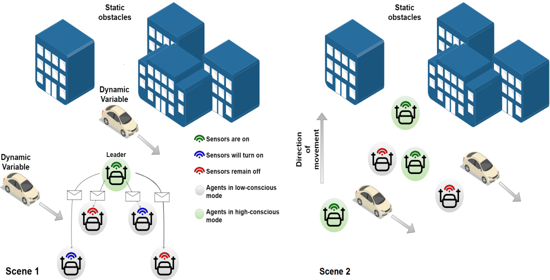
In a multi-agent system, it is a norm to have every single agent making more or less intelligent decisions by utilizing the onboard sensor system for observing the surroundings. The active sensors and onboard processing of sensory data consume power and reduce battery run-time, which results in decreased mission life on a single charge. However, in static environments, all of the agents in the swarm do not necessarily have to either keep their onboard sensors turned on continuously or take decisions intelligently. If intelligent decision making and sensor usage are restricted based on some constraints, depending on the environment and surroundings, a major portion of power consumption due to sensors and related data processing can be reduced, as shown in
Figure 1. The approach that is presented in [
17] proposes a translational coordinates scheme in which the leader agent has its sensor turned on all the time, while the follower agents turn on their sensors as soon as the leader detects any static obstacle in its surroundings. Indeed, for such environments, if only the leader of the swarm remains at a high-conscious mode continuously and performs all of the necessary required calculations (
Figure 1a), the system’s sensor related power consumption can be reduced considerably, and the potential run-time of the mission is thereby increased. Furthermore, the adaptive capability of the individual follower agents to dynamically switch between the low-conscious and autonomous high-conscious modes, depending on the situation at hand (
Figure 1b), guarantees that the system’s degree of autonomy is not compromised.
In this paper, based on the principle that is described above, an approach is developed to reduce the overall power consumption of the system by intentionally deactivating and reactivating the sensors at run-time. Basing our proposed technique on reactive agents [
6] and a control methodology for formation based on 1-N leader-follower approach (1-leader and N-followers) [
38], the leader constantly observes the environment and informs its followers of the coordinates of any detected obstacles in the vicinity. In case there are no obstacles in the vicinity of the leader, it only broadcasts its own coordinates. The follower agents, after translating the coordinates according to their own positions, decide whether continuing the same trajectory is safe or if they are required to deviate from their path. However, in the case a dynamic obstacle is detected by the leader agent, the coordinates are broadcasted in a similar manner to the followers, who, then upon performing the necessary calculations, realize the direction of movement of the obstacle and its speed. After this, based on their own trajectory and the obstacle’s trajectory, it is calculated if continuing on the same trajectory will lead to a potential collision, in which case the respective agent switches from the low-conscious mode to the autonomous high-conscious mode, as shown in
Figure 1. After successfully avoiding the collision or bypassing the obstacle, the follower agent switches back again to the low-conscious mode. Individual agents in the swarm utilize the collision avoidance technique developed and presented in [
9] for avoiding collisions in the high-conscious mode. The main motivation behind this approach is not only the overall power cost reduction of the swarm, but also the capability of the agents to autonomously decide on switching between the low-conscious and high-conscious modes, enabling situation-aware optimization of power consumption, due to ranging sensors, at run-time. A simplified approach has been chosen for validation of the proposed approach by limiting the depth of the swarm to two agents, i.e., ”N” = 2 agents in the 1-N leader–follower model. It is important to note here that the agents in the Follower_Mode are assumed to utilize the on-board IMU (Inertial Measurement Unit) and GPS (Global Positioning System) for localization purposes, i.e., obtaining their own positions (localization methodologies are not in the scope of this work. However, while in low-conscious mode, the possible error in obtaining position vectors due to the IMU drift over time and also the probable GPS signal loss, is also handled by the algorithm, as the cross-checking of the translated coordinates will return false readings and the follower agent will go into the high-conscious mode temporarily).
3. Proposed Approach
In this section, we describe the proposed method in more detail. The strategy is to combine the navigation and object detection with coordinate calculation and adaptive autonomous modes in order to facilitate the process of autonomous swarm navigation using translational coordinates. The proposed top-level algorithm to accomplish this (Algorithm 1) is composed of two partial feedback-based algorithms: one for managing the followers and the other for managing the adaptive autonomous mode in the presence of obstacles. The adaptive autonomous mode calls collision avoidance from within if deemed to be necessary.
In the Follower_Function module, drones receive the coordinates of their leader and of the obstacles, as seen and transmitted by the leader, and then perform the necessary calculations to translate the received coordinates according to their own respective positions. Meanwhile, if there is no feedback from the leader and the defined timeout is exceeded, it is assumed that the leader is not alive/reachable, i.e., the communication link with the leader is lost. In such a case, the drone in question temporarily declares itself as its own leader as a fail-safe mechanism and resumes navigation by turning its sensors on.
The environment is declared to be dynamic, if the leader detects one or more moving obstacles, or if the cross-check of the translational coordinates indicates a mismatch. The follower, in this case, starts calculating the obstacle’s velocity to determine the apparent point of impact. Upon estimating the point of impact, the follower node/drone itself decides when it needs to turn on its sensor(s) in order to perform active collision avoidance for safe maneuvering.
| Algorithm 1 Leader: Navigation & Object Detection |
| agent Leader() |
| 2: while True do |
| if obstacle detected then |
| 4: , ← Obstacle’s distance and angle calculation; |
| end if |
| 6: for all i do |
| Follower(i).Transfer_Coordinates(); |
| 8: if then |
| ← Reverse cross-check follower’s received |
| coordinates(); |
| 10: ← Reverse cross-check follower’s received angle(); |
| = , ; |
| 12: if || > OR || > then |
| Follower(i).Set-Dynamic; ▹ Setting remote Dynamic flag |
| 14: end if |
| end if |
| 16: end for |
| Collision_Avoidance(); |
| 18: end while |
| end agent
▹ end agent leader |
3.1. Agent Leader
Algorithm 1 provides the general pseudo-code for the global leader. This top-level algorithm is executed utilizing the on-board processing units by all agents locally. The assignment of IDs to all agents is assumed to be achieved before starting the mission. The algorithm is initialized by first setting up the necessary flags. Subsequently, the leader agent starts scanning for any obstacles in the vicinity and then calculates the distance and angles at which the detected obstacle(s) lie (Lines 3–4). After this, the leader starts sending its coordinates to its respective follower(s), including the detected obstacle’s (if any) angle and distance (Lines 6–7). Here, the symbols, and , are used to simplify the notations and contain the distance of the obstacle(s), the angles at they lie, the agents’ own parameters, such as coordinates and heading direction. After receiving the coordinates from its follower(s), i.e., the transfer is successful (), the leader cross-checks the distances and angles calculated by the follower (Lines 8–10). After cross-checking, the environment is declared to be dynamic if the absolute value of the received angles or coordinates, i.e., , is more than a defined threshold level, i.e., error tolerance for coordinates and error tolerance for calculated angle (Lines 12–14). The leader agent then calls Collision_Avoidance to bypass the obstacle(s) successfully (Line 17).
3.2. Agent Follower
Algorithm 2 provides the general pseudo-code for the follower agents. The algorithm starts by declaring its global procedures that are also utilized by the leader and, furthermore, setting up the necessary
flags (Lines 2–3). Afterwards, the follower agent(s) check if the leader is alive, i.e., they are getting constant feedback from the leader (
Lead_is_Alive == True), or if they are in the follower mode, i.e.,
Follower_Mode == True. If either
Lead_is_Alive or
Follower_Mode is False, the respective agent performs obstacle detection actively and then calculates the distance and angle at which the obstacle is detected (Lines 5–6). In the case of constant feedback from the leader, the respective follower agents check if the environment has been declared as dynamic by the leader or not. If the environment is not declared as dynamic, the agent calls
Follower_Function for navigational purposes. On the contrary, if the environment has been declared to be dynamic,
Adaptive_Mode_Function (Lines 8–11). Finally, the
Coordinates_Received flag is reset to False, for next iteration (Line 13).
| Algorithm 2 Follower: Navigation & Object Detection |
| agent Follower() |
| 2: global procedure Transfer_coordinates, Set-Dynamic;▹ declaration of of follower’s |
| global procedures Leader will call |
| = True, True, False, |
| False; |
| 4: while True do |
| if (! OR !) AND obstacle detected then |
| 6: , ← Obstacle’s distance and angle calculation; |
| end if |
| 8: if ! AND then |
| Follower_Function(); |
| 10: else |
| Adaptive_Mode_Function(); |
| 12: end if |
| = False; |
| 14: end while |
| end agent ▹ end agent follower |
3.3. Set-Dynamic
Algorithm 3 shows the procedure that is called by the leader to set the dynamic flag for its followers to True.
| Algorithm 3 Set-Dynamic |
| procedure Set-Dynamic() ▹ this procedure is called remotely to set Dynamic to True |
| for Follower(i) |
| 2: = True; |
|
end procedure |
3.4. Transfer Function
Algorithm 4 specifies the pseudo-code for Transfer Function. The algorithm starts by setting the
, i.e., the transfer success, flag based on the
and randomizing the True/False to simulate the possibility of transfer failure (Line 2). Subsequently, if
is True, the data sent by the leader are utilized to compute the translated coordinates by the follower (
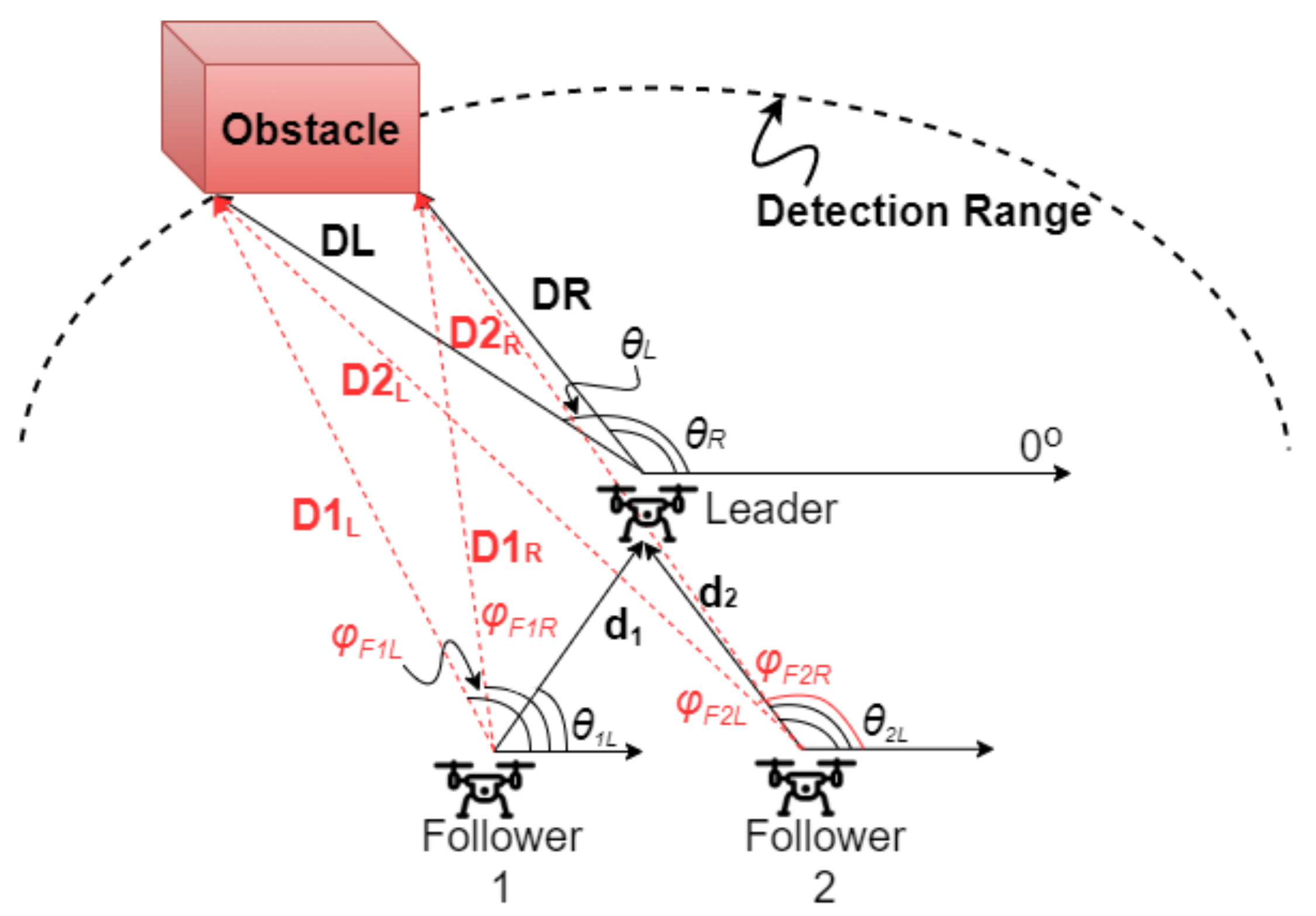
). If there was a constant feedback from the leader, the node/follower uses the translational coordinates of the obstacle, as observed by the leader and based on its own coordinates, calculates the location of the obstacle according to its own position, as shown in
Figure 2 variables description given in
Table 1). These translated coordinates that are calculated by the follower are then utilized by the leader, as data from the follower,
, (Algorithm 1, Lines 17–19) for cross-checking purposes. The
coordinates_received flag is then set to
True (Lines 3–6).
| Algorithm 4 Transfer Function |
| procedure Transfer_Coordinates() |
| 2: = ! AND random select(True, False);▹ modeling transfer |
| failure possibility |
| if then |
| 4: = ; |
| = calculate translational coordinates(); ▹ Follower’s data for Leader |
| 6: = True; |
| = True; ▹ if is False, turn it to True |
| 8: end if |
|
end procedure |
3.5. Follower Function: Coordinate Calculation
Algorithm 5 specifies the
Follower_Function module, where the follower node waits until either the defined
Timeout is reached or the coordinates are received (Line 2). Subseuently, if the
coordinates_received is True, i.e., coordinates are received by the follower, the reference coordinates that the follower should navigate to, i.e.,
ref.coords, are updated w.r.t.
(Lines 3–4). Moreover, if the ranging sensors are on/activated previously, they are turned off, as the agent is now in the follower mode (lines 5–6). However, if the coordinates are not received until the
Timeout, the
Lead_is_Alive is set to
False, ranging sensors are turned on for actively observing the environment and perform obstacle avoidance, and to make itself its own leader, the node sets the
ref.coords as its own coordinates, i.e.,
self.coords, to start navigating towards the destination (Lines 8–11).
| Algorithm 5 Follower Function |
|
procedure
Follower_Function()
|
| 2: wait until OR ; |
| if then |
| 4: ←;▹ Update the reference coordinates to translational coordinates |
| if Sensors are ON then |
| 6: Turn off the Sensors; |
| end if |
| 8: else |
| = ; |
| 10: Turn on the Sensors; |
| = ; |
| 12: end if |
|
end procedure |
The timeout signal is only checked if the node in question is not the leader itself. Every other node constantly checks whether its respective leader’s transmitted signals are being constantly received. If the node has not received the coordinates sent by its leader by the timeout, it turns on its sensors for active collision avoidance maneuvering by declaring itself as its own leader.
3.6. Adaptive Mode Function
This module, Algorithm 6, is called by the leader if it detects obstacles in the vicinity. Or, in the case the environment is already as dynamic, then the nodes in
Follow_Mode call this module locally. As soon as this module is called, it is checked whether the node in question is the global leader or is it one of the followers (Line 2). The default or initial value of
Follow_Mode for all of the follower nodes is
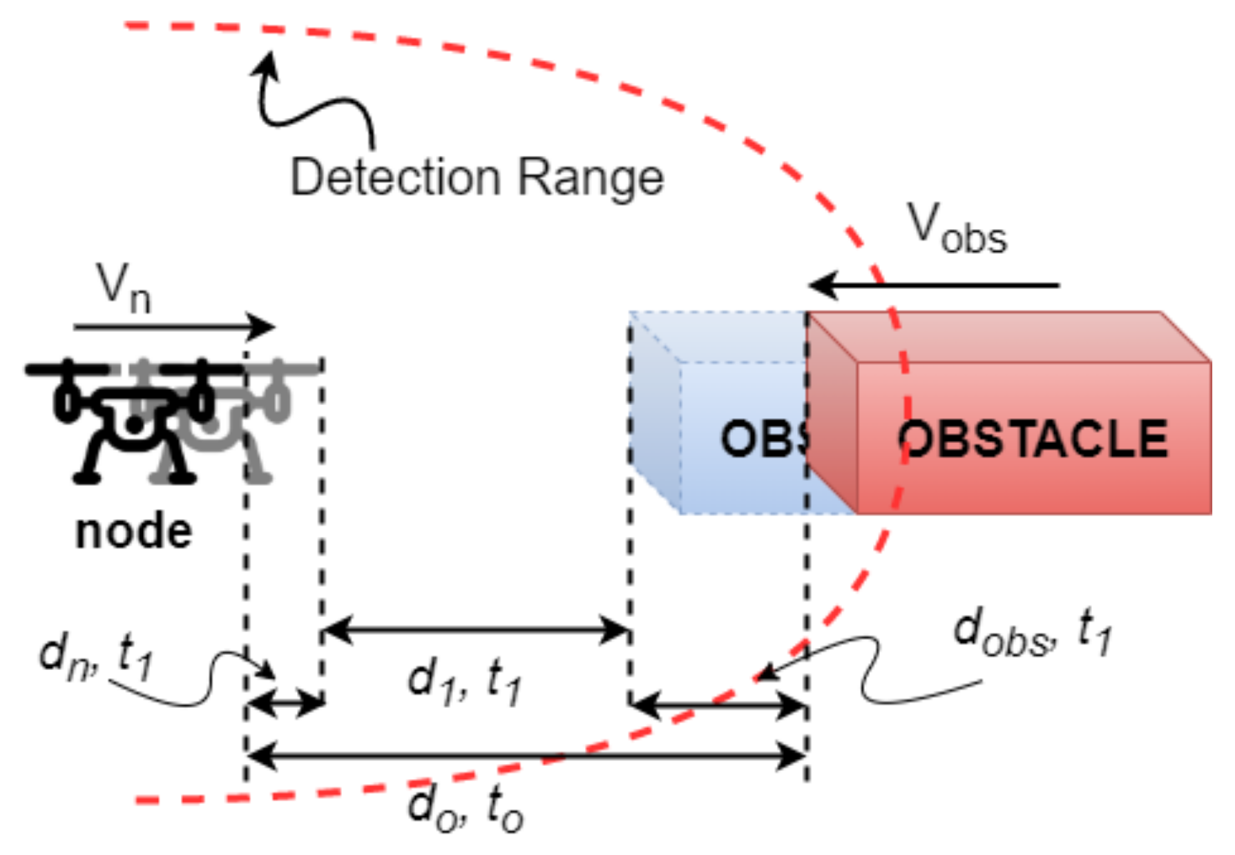
True. If the node is the follower, using previous translational readings, the obstacle’s velocity is approximated (Line 3) using Equations (1)–(3), and a visual illustration is shown in
Figure 3.
| Algorithm 6 Adaptive Mode Function |
|
procedure
Adaptive_Mode_Function()
|
| 2: if then |
| ← Calculate obstacle’s velocity from previous readings(); |
| 4: ← Calculate the distance to impact; |
| if < Detection Range then |
| 6: Turn on the sensors; |
| = ; |
| 8: end if |
| end if |
| 10: Collision avoidance (); |
| if NOT in Detection Range then |
| 12: = ; |
| if != AND then |
| 14: = ; |
| Turn off the sensors; |
| 16: end if |
| end if |
| 18:
end procedure |
Three scenarios are possible based on
: (1) if
< 0, i.e., positive, this means that the obstacle is going away from the node; (2) if
= 0, this means that the obstacle is not moving, i.e., stationary; (3) if
< 0, this means that the obstacle is travelling towards the node. Based on these readings, the distance to the potential impact/collision (
) is calculated (Line 4). The distance travelled by the node after
seconds is computed by:
where
and
are the distances travelled by the node and velocity of the node, respectively. The distance covered by the obstacle and its velocity can be determined by (2) and (3), respectively:
where
is the distance travelled by the obstacle,
velocity of the obstacle,
the distance travelled by the node,
the distance between the obstacle and the node at time
, and
is the distance between the obstacle and node at the previous time
.
If the distance that is travelled by the obstacle is zero, i.e.,
= 0, it means that the obstacle is stationary. However, if the distance covered by the obstacle after
, i.e.,
is less than the distance between the node and the obstacle (
), in that case, the obstacle is moving towards the node (as shown in
Figure 3). Otherwise, the obstacle is moving away from the node. Based on the movement of the node and the obstacle, the apparent distance to impact is calculated and, if that distance to impact is less than the detection range of the on-board sensor system, the node turns on its sensors and comes out of follower mode to perform active collision avoidance (Lines 5–7). The collision avoidance module is then invoked to constantly monitor the environment (line 10). After successful collision avoidance, the status of the surroundings is changed back to static (Lines 11–12). The node turns off its sensors and goes back into
Follow_Mode and the control is returned to the main module (Lines 13–16).
3.7. Collision Avoidance
Collision avoidance, with the pseudo-code in Algorithm 7, is invoked when the detected obstacle gets critically close. It is then checked whether there is only one obstacle in the vicinity or there are multiple obstacles (Line 3). In case, more than one obstacle is detected, the gap between the obstacles is calculated (Line 4). Based on the calculation, the algorithm takes the following actions: if the
is more than the
, i.e., defined based on the dimensions of the UAV, then the UAV is aligned to pass through the gap available between the obstacles (Lines 5–6); otherwise, the obstacles are treated as a single obstacle and the UAV is rerouted accordingly to navigate around them in order to avoid collisions (Lines 7–9). However, if only one obstacle was detected in the first place, the path planning is done accordingly to bypass the obstacle while keeping the deviation to a minimum (Lines 11–13). For performing successful path planning and aligning, we utilized and implemented the technique that is presented in [
9]. The algorithm then recalculates the obstacle’s distance and updates it. Based on the updated value, the control returned back to the Adaptive_Mode_Function.
| Algorithm 7 Collision Avoidance |
|
procedure
Collision_Avoidance()
|
| 2: while < Detection Range do |
| if detected obstacles > 1 then |
| 4: ← calculate the gap between obstacles; |
| if > then |
| 6: path planning(edges); ▹ UAV is aligned to pass through the obstacles |
| else |
| 8: ← single obstacle; |
| path planning(path_plan); ▹ considered as single obstacle |
| 10: end if |
| else |
| 12: ← single obstacle; |
| path planning(path_plan); |
| 14: end if |
| ← Update the obstacle distance; |
| 16: end while |
|
end procedure |
4. Simulation Results
The area used for the basis of the simulation was defined as 700 m × 500 m two-dimensional XY-plane, i.e., all of the objects are considered to be at the same altitude. The number of agents is set to three and the agents are already in the defined V-shaped formation at the start of the mission. It is important to note that, in the performed experiments, the leader agent has more computational and power resources to be able to perform the leadership tasks. The leader was equipped with Nvidia Jetson TX2, which is a power-efficient embedded system with the capability of operating between 0.5–2 GHz. In order to be more power efficient, we set the operating frequency to 0.5 GHz, at which the average power consumption is 4.5 Watts. The followers were equipped with Raspberry Pi 3B, which consumes around 2.4 Watts in high-conscious mode and 1.4 Watts in the idle mode. Velodyne Puck LITE was used for the generation of the data, which was then used in the simulation platform for visualization purposes, simulating the sensor, generating the obstacles, and subsequently to verify the proposed algorithm. Puck LITE has a 360
field of view horizontally, 30
vertically, generates 300,000 points/second, and has an accuracy of ±3 cm and range of 100 m [
51]. For communication between the agents, due to its longer transmission range (100 m indoor/urban environment), data rate of 250 kbps, and possibility of large number of devices to be connected, communication-based power consumption is evaluated based on Legacy Digi XBee-Pro S1 802.15.4 consumption, i.e., in Transmitting Mode = 710 mW, in Receiving Mode = 182 mW [
52].
The following assumptions and initial conditions are used in this study:
all of the agents are travelling with constant ground speeds;
communication link between the agents is setup ideally and with no information loss; and,
agents utilize the on-board localization techniques in order to obtain their positions.
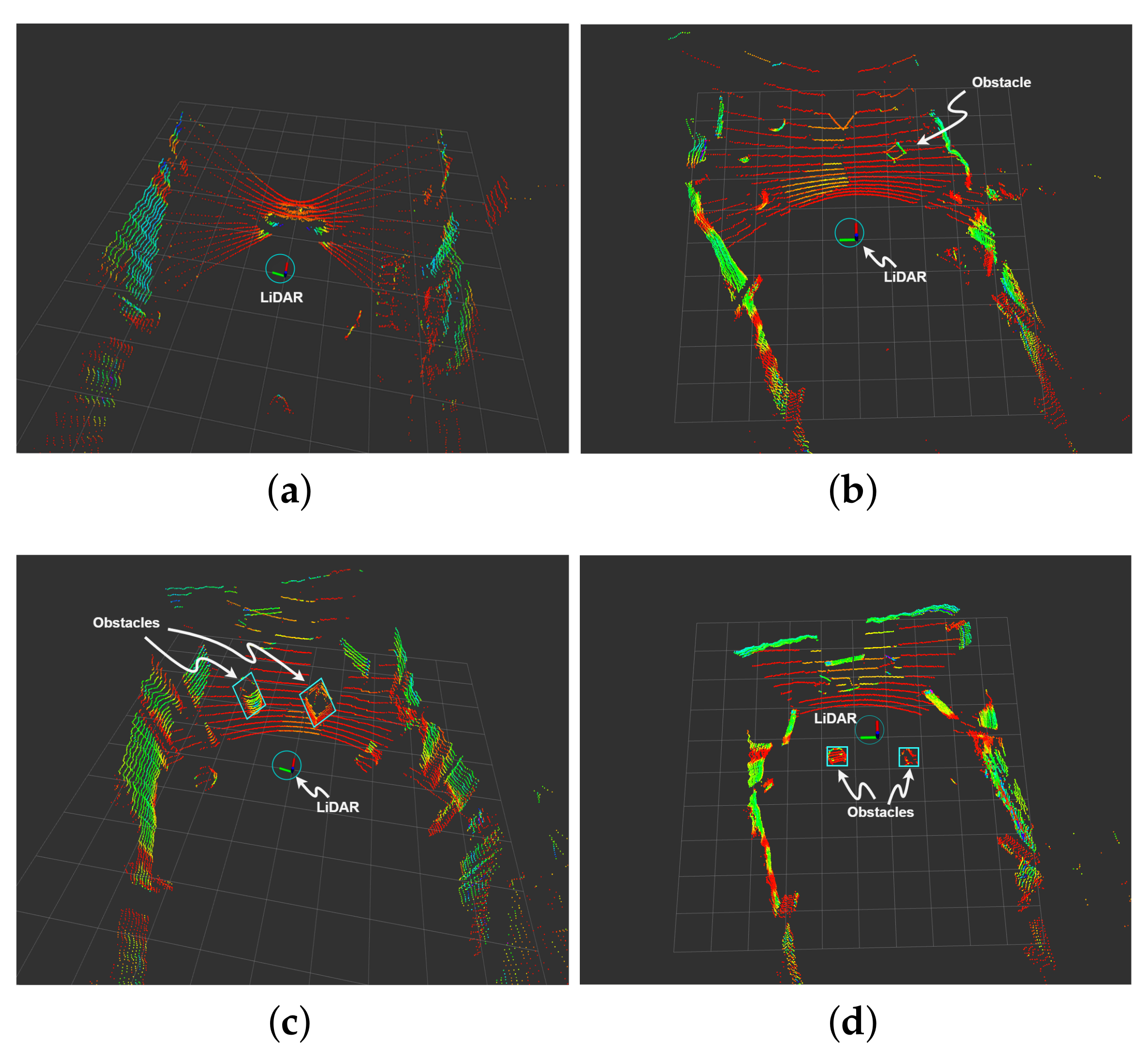
The LiDAR (Light Detection and Ranging) data [
53] is shown at different time intervals and from different angles shown in
Figure 4.
Figure 4b–d show the obstacles when they are in close vicinity and in the detection range. These figures show the position of the LiDAR sensor equipped drone as the blue, red, and green interactive marker. It is to be noted that the developed algorithm takes the point cloud that is captured by the LiDAR based on the defined constraints to reduce the complexity of the algorithm. Because its running on a resource-constrained system it is crucial to discard unnecessary point clouds, i.e., point clouds that are not in the field of view (FoV). The FoV is defined in the proposed algorithm to be ± 30
. Only the obstacles within this FoV are considered to be posing a potential collision threat to the agents and, therefore, any obstacles outside this are discarded. The detected obstacles are contoured by light blue rectangles.
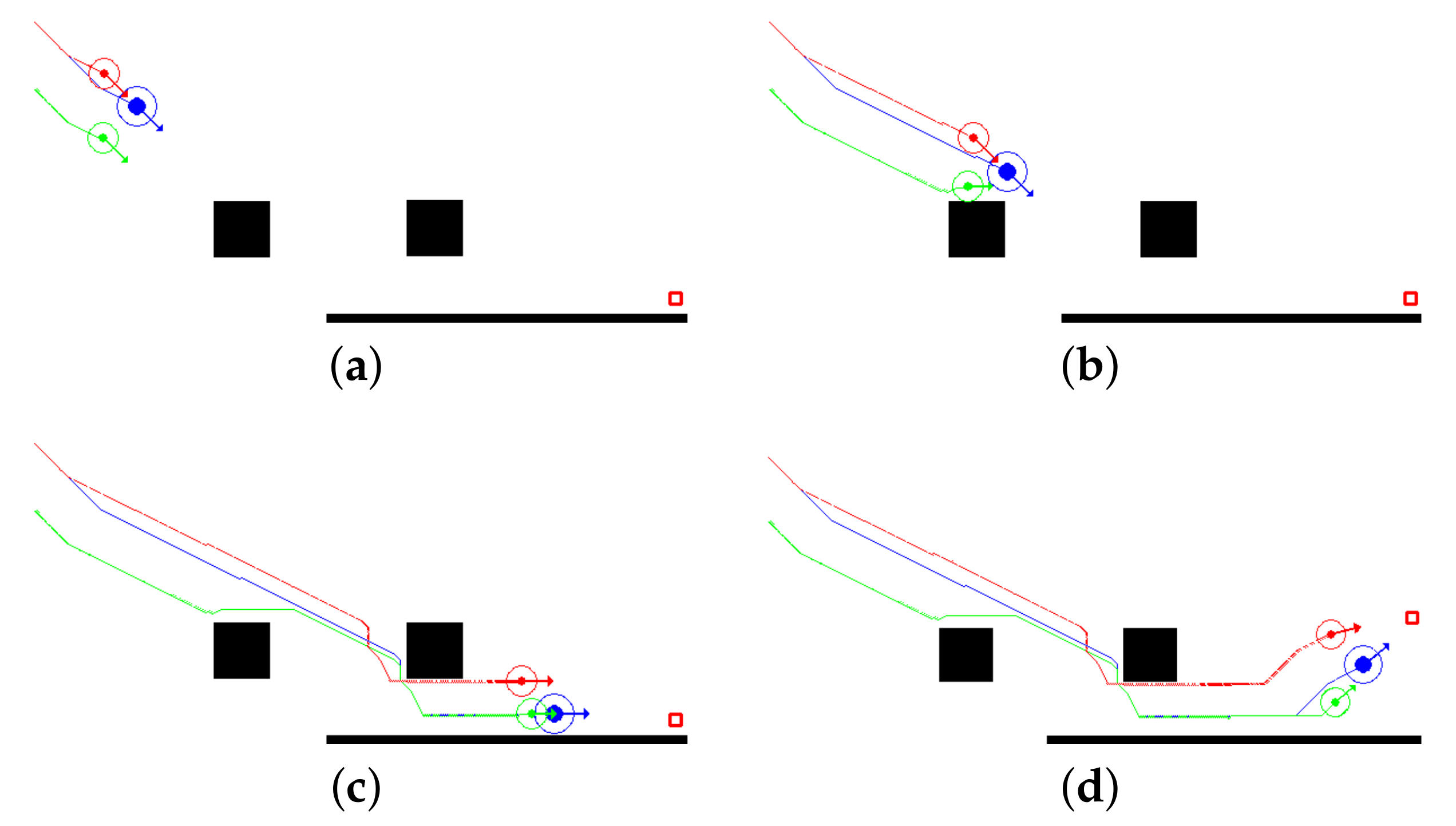
Figure 5 shows the simulation results for a static environment when the obstacles are stationary. In the V-shaped formation that is shown in the figure, agent 1 (leader) is shown as a blue circle, which has its ranging sensor (shown in
Figure 4) on always-on mode, while red and green followers, i.e., agent 2 and agent 3 respectively, are following the leader by translating the leaders’ transmitted coordinates as shown in
Figure 2. In
Figure 5b, the obstacle has entered the detection range of agent 1 but since there is no danger of collision, agent 1 continues its trajectory as shown in
Figure 5c. Similarly, agent 2 is following agent 1 while utilizing the translational coordinates, and as there is no collision risk found upon calculations it continues to function in the
Follower_Function. Whereas, as shown in
Figure 5b, the translational coordinates calculations performed by agent 3 clearly indicate the potential collision if the same trajectory is continued and, therefore, it diverts from its original trajectory by performing offline collision avoidance to avoid the obstacle, as can be seen from the traces of the agents in
Figure 5c.
Agent 2 maintains its trajectory w.r.t. the leader without deviating from the original trajectory even while going through the obstacles and second obstacle being close to it, as can be seen from
Figure 5c,d. This shows the effectiveness of utilizing the translational coordinates as the obstacle was out of the collision radius as also indicated by the performed calculations by the agent. Whereas, agent 3 maintains the pre-defined minimum distance from agent 1 after avoiding the obstacle, which is due to the third obstacle in the bottom. In
Figure 5d, the destination point was moved at run-time to demonstrate the reformation process and, as can been seen, agent 3 starts going back to the position in the formation, it was supposed to be, as soon as it moves away from the obstacle in the bottom.
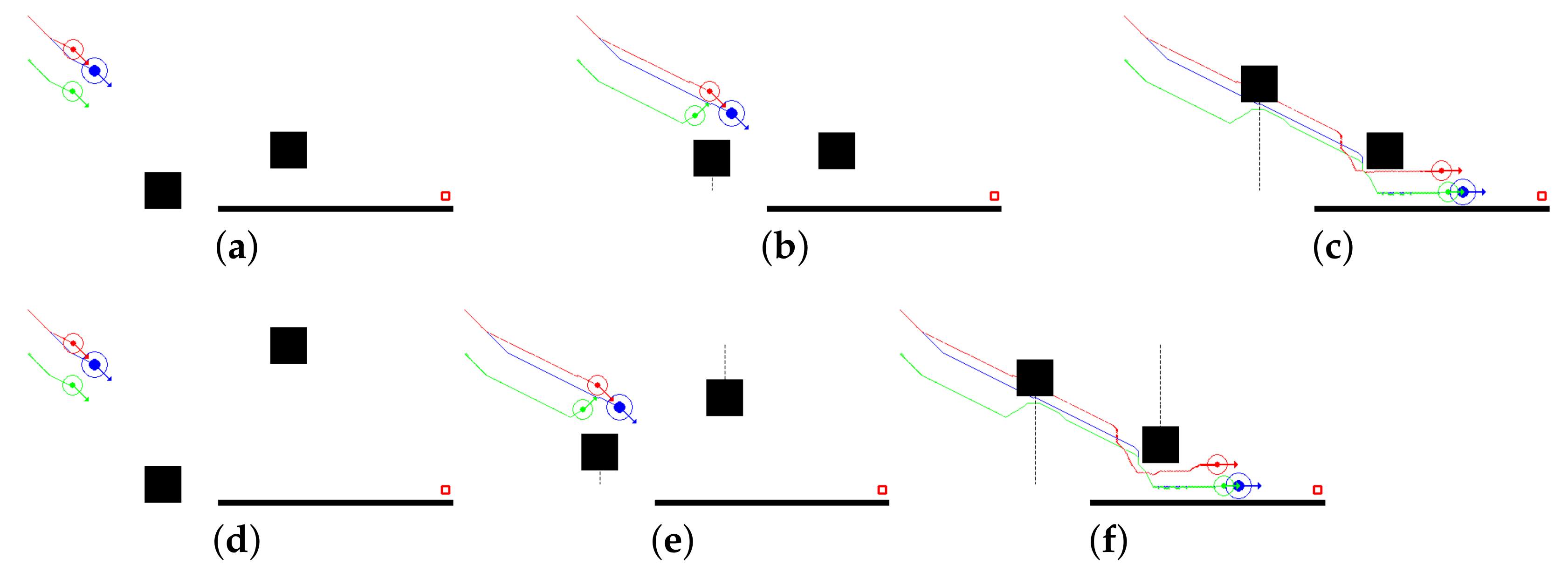
Figure 6 illustrates the simulation results for dynamic environment scenarios, where:
Case 1: only one obstacle is moving, as shown in
Figure 6a–c. In this case scenario, the obstacle is moving in the direction of the swarm. The obstacle, as observed by agent 1, will intercept the swarm and a potential collision is evident if agent 3 continues its trajectory, as can be seen from
Figure 6b. Therefore, after performing the necessary calculations, agent 3 turns on its own ranging sensor and performs collision avoidance actively. After avoiding the obstacle, agent 3 turns off its sensors and starts following the leader once again based on translational coordinates from the leader.
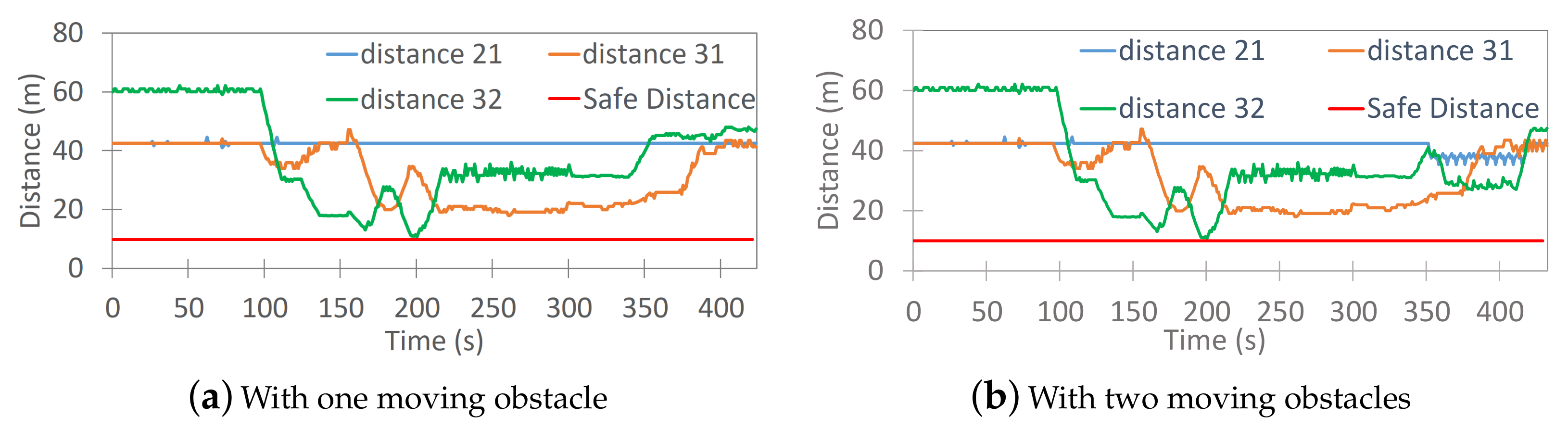
Figure 7a shows the distance maintained by the agents throughout the simulation;
Case 2: two obstacles are moving, as shown in
Figure 6d–f. In this case scenario, the first moving obstacle only disturbs agent 3, as in Case 1. However, after performing the translational coordinate calculations, as soon as agent 2 observes that the second obstacle is moving towards their direction and a collision may be inevitable, it turns on its ranging sensor to actively avoid the collision and divert from its trajectory if necessary (as shown in
Figure 6f). After successful avoidance, when there are no moving obstacles in the vicinity, the agents turn off their sensors and switch back to the
Follower_Function.
Figure 7b shows the distance maintained by the agents throughout the simulation.
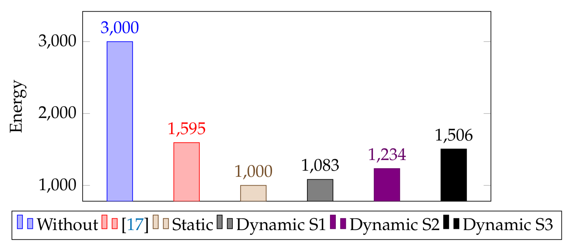
We report and compare the power consumed by our setup based on the experiment to analyze the efficiency of the proposed algorithm. The battery used in the setup for calculation of these attributes was 5000 mAh and, in typical conditions, the power consumption of one Velodyne Puck LITE is 8 Watts and operating voltage is 9 volts. Based on these values and the tracking the amount of time, each agent had its sensor turned on during the simulation with and without our proposed methodology, as shown in
Figure 8. We placed these calculated values side-by-side with the reference algorithm [
17]. The normal setup with all agents running their sensors always-on mode will consume about 3000 mWh, which is calculated as
where the summation is over all the agents in the system,
denotes the energy consumption of an agent,
is the power consumption of the agent’s sensor, and
is the total time for which the agent’s sensor remains active. In the instant case, there are three agents, the power consumption of the sensor is 8000 mW and the sensors remain active all the time, i.e., 450 s,
comes out to be 1000 mWh and the total consumption for three agents will be 3000 mWh.
Similarly, the setup that was used in [
17] consumed 1595 mWh, as in that setup the follower agents turn on the sensors as soon as the leader detects any static obstacle. However, while utilizing the proposed modified algorithm, the energy consumption for the same setup can be reduced by about 600 mWh to 1000 mWh. As in the proposed methodology, only agent 1 (the leader) had its sensor always-on, while agents 2 and 3 never had to turn on their sensors, as they only translated the broadcasted coordinates by the leader and followed. Subsequently, the power consumption due to ranging sensors in static environments can be further reduced by another 40% mark approximately. Additionally, that can be further utilized when the environment has some dynamic variables involved and, hence, increasing the overall mission life on a single charge. When testing the proposed methodology for the environment with some dynamic variables, the following results were observed: (1) Dynamic S1: is the experiment with swarm consisting of three agents and obstacle 1 moving. This only affected agent 3, and agent 3 turned on its sensor to perform collision avoidance for 37s and turned off the sensor after successful avoidance to go back into the
Follower_Function resulting in the overall energy consumption due to sensor usage by all nodes to 1083 mWh; (2) Dynamic S2: is the experiment performed with swarm that consists of three agents and obstacle 1 and 2 are both moving. This affects both agents 2 and 3. Agent 3 had to turn on its sensor for 37 s, while agent 2 had its sensor turned on for 68 s, which resulted in the overall energy consumption due to sensor usage by all nodes to 1234 mWh; and, (3) Dynamic S3: is the experiment performed with swarm consisting of five agents and both obstacles 1 and 2 are dynamic. This affects all of the agents. Agents 2 and 3 remain at high-conscious mode for the same amount of time as in “Dynamic S2” case, whereas agents 5 and 4 remain at high-conscious mode for 57 s and 65 s, respectively. Resulting in the overall energy consumption due to sensors usage to 1506 mWh.
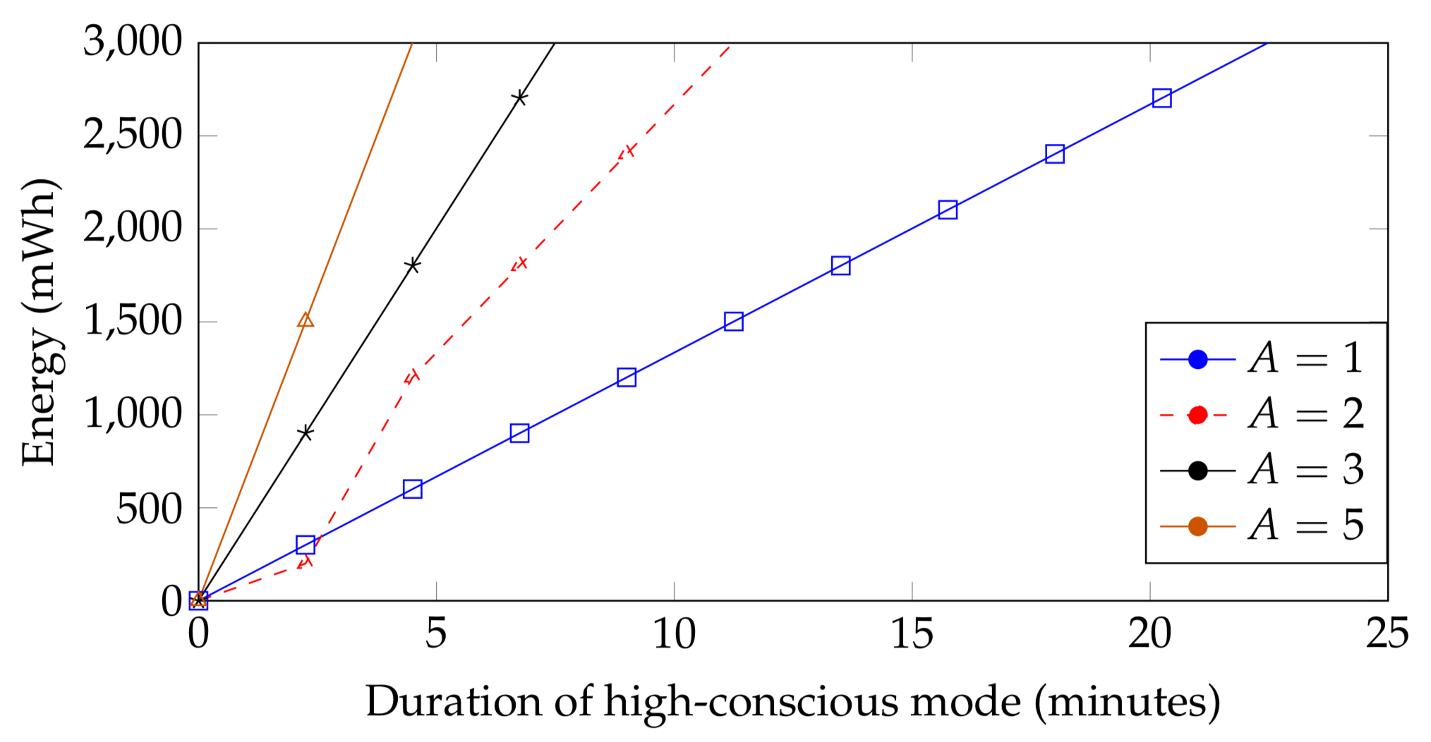
Based on the incremental consumption due to dynamic obstacles in the environment,
Figure 9 shows an estimation of the relationship between the dynamicity of the environment and the energy consumption of the swarm. It is important to note that the energy consumption due to the sensor(s) usage depends on the duration that each agent stays at the high-conscious mode. It can be concluded that the energy consumption of the swarm is independent of the number of dynamic obstacles; however, it is dependent on the duration that each agent is affected by the dynamic obstacles or has to stay at high-conscious mode, i.e., their sensor(s) turned on. In the figure,
represents one agent operating in high-conscious mode,
represents two agents operating in the high-conscious mode,
shows the consumption of the swarm when three agents are operating in the high-conscious mode, and
shows the consumption of the swarm when five agents are operating in the high-conscious mode.
5. Conclusions and Future Work
We developed an algorithm for a pre-defined formation of multi-agents with adaptive ability for static and dynamic environments to reduce the power consumption due to sensors usage. Under normal conditions in a static environment, one dedicated agent (leader) can see its surroundings with the sensors turned on, while other agents (followers) blindly follow by translating the received coordinates from the leader. However, according to the demand of the environment, the follower(s) have the ability to decide to turn on their ranging sensors for safe maneuver, after performing the necessary calculations. The proposed methodology of the effectiveness of translational coordinates and the proof of concept was verified in the simulation environment. It is evident from the simulation results that the proposed method is reliable in static environments, as well as in the environment with some dynamic variables. Furthermore, it helps in reducing the power consumption due to the usage of sensors over time. The proposed method, in the considered test case and static environment, helped in reducing the power consumed by the sensors by about 40% when compared to the reference algorithm. In general, it is obvious that this power saving in dynamic environments definitely depends on the structure of the environment and its dynamicity. However, in environments with some dynamic variables in our test scenarios, the proposed methodology still proved to be effective, as utilizing it kept the power consumption about 50% less than if the sensors were used in a continuous mode.
In the future, we plan to further extend this work by increasing the depth of the swarm, i.e., the number of followers in the swarm, in order to further investigate the information exchange between the agents by taking the possible communication delays into consideration. Furthermore, the power consumption due to wireless communication and the effect of processing the information and coordinates on the battery life will also be analyzed. Because the leader undertakes all of the necessary computations, leading to faster draining of its battery and resultant shortening of overall life time of a mission, it will be interesting to analyze the effectiveness of an election-based leadership solution and explore different options for optimally swapping the leadership role amongst the followers, e.g., swap the places by selecting the follower with highest remaining battery life. Further, the effect of such improvements on the overall mission life needs to be studied. Additionally, finally moving onto testing the proposed approach in real-time initially under static environments and further moving to real-time controlled dynamic environments.


 ,
, 


