Abstract
In the current alteration of temperature and snow cover regimes, the impacts of winter climate have received considerably less attention than those of the vegetation period. In this study, we present the results demonstrating the influence of the winter climate conditions on the Mountain pine (Pinus mugo Turra) communities in High Tatra Mts (Western Carpathians). The changes in greenness in 2000–2020 were represented by the inter-annual differences of satellite-derived Normalized Difference Vegetation Index (NDVI). The winter climate conditions were characterized by climate indices calculated from the temperature and snow cover data measured at Skalnaté Pleso Observatory (1778 m a.s.l.) over the period between 1941–2020. Areas with P. mugo were classified into two density classes and five altitudinal zones of occurrence. The partial correlation analyses, which controlled the influence of summer climate, indicated that winter warm spells (WWS) caused a significant decrease in the greenness of the P. mugo thickets growing in the dense class D2 (R = −0.47) and in the altitudinal zones A2 (1600–1700 m a.s.l.) and A3 (1700–1800 m a.s.l.) with R = −0.54 for each zone. The changes in greenness were related to the average snow depth (ASD) as well, particularly in the dense class D2 (R = 0.45) and in the altitudinal zone A2 (R = 0.50). Here, in the summers following winters with the incidence of WWS or low ASD, we found decreased greenness following the injury of P. mugo shrubs, but NDVI after winters with higher ASD indicated more greenness. At lower altitudes, injuries may result in the loss of competition capacity of P. mugo near the timberline, where taller mountain tree species can utilize the conditions of warmer climate for expansion. We also found a significant positive effect of warmer winter seasons in the sparse P. mugo thickets (D1) with R = 0.50 and at higher altitudes (R = 0.49 in A4—1800–1900 m a.s.l.; R = 0.53 in A5—1900–2000 m a.s.l.). The increased temperatures in December correlated significantly with the increase of the greenness in all P. mugo pixels (R = 0.47), with the most pronounced effect in the sparse class D1 (R = 0.57) and in altitudinal zones A4 (R = 0.63) and A5 (R = 0.44), creating advantageous conditions for the thermophilisation of the alpine zone by P. mugo.
1. Introduction
Mountain and alpine ecosystems cover more than 20% of the Earth’s land surface spanning over areas from the equator to just near the poles [,]. P. mugo is native to central and southeast Europe, ranging from the Swiss-Austrian border in the Alps to the Ore Mountains (eastern Germany, Czech Republic), the Carpathian Mountains (Slovakia, Poland, western Ukraine) and through Croatia and Romania to Bulgaria, with western outliers to the Vosges and French Alps and an isolated population in the central Italian Apennines []. In most of these mountains, the P. mugo shrubs form a coherent, climatically conditioned vegetation belt, mostly known as a subalpine belt near the timberline []. The subalpine belt refers to an intermediate zone between the mountain and alpine vegetation with an ecotone character []. P. mugo reaches higher altitudes than any other conifers (up to 2400 m). In Holocene, in the Western Carpathians and Hercynian region, it was pushed by spruce and beech to higher altitudes (above 1250–1500 m a.s.l.), and eventually to peatlands and rocky mountains. The presence of symbiotic fungi on the pine roots enables this scrub to procure the nitrogen component of nutrients and thereby enables P. mugo to survive in places where other tree species reach their limits []. Towards the upper limit, populations of P. mugo gradually become lower and more prostrate []. Its spatial spread depends not only on seed dispersal and on germination, but the horizontal spread is also supported by vegetative reproduction [] by forming multi-stemmed clones (polycormones) [].
Current alteration of temperature, precipitation and snow cover regimes as a consequence of climate change may lead to disturbing and weakening of the mountain ecosystems that provide important ecosystem services. The amplified warming in high-elevation areas [,,] corresponds with the rising global temperature [,]. As a consequence of the warming, evaporation and atmospheric humidity increase. In high mountains, this may lead to more frequent and rich snowfalls but concurrently to the reduction of the snow season duration and earlier melting [,]. Whether the amount of snow on the ground will be reduced or increased depends on the balance between these competing factors []. In the northern hemisphere, snow cover is likely to migrate northward in the future with higher loss rates in northern latitudes (45°–49°N) and at high elevation [], particularly in spring and summer seasons []. In spite of this global trend, the trends in snow conditions are variable on regional scales [], depending on the topographic features (elevation, aspect and terrain shading), orography and the proportions of occurring synoptic situations. The potential for vegetation injury in winter is considerable, given by the loss of snow cover, which exposes plants to sub-zero ambient temperatures and large temperature fluctuations leading to damage by winter desiccation. Freeze–thaw cycles and abrasion of needles and sprouts by windblown ice particles damage the vegetation before fresh snow covers it repeatedly [,,]. The occurrence of extreme winter warming events that can cause major damage to subalpine plant communities at landscape scales [] has become more frequent over the last decades []. In the high mountain ecosystems, even small but recurring disturbances caused by climate warming may lead to thermophilisation, when the more cold-adapted species decline and the more warm-adapted species increase [,].
We processed the satellite data from the MODIS (Moderate Resolution Imaging Spectroradiometer) from 2000 to 2020 to derive the NDVI (normalized difference vegetation index) for the P. mugo subalpine belt. The employment of satellite data provided the opportunity to shift from in situ observations to large-scale analysis. The NDVI provides the index of vegetation greenness related to aboveground net primary productivity []. Previously, it has been successfully used as input to develop measurements of the biophysical properties of ecosystems [,,,,,]. We described the inter-annual variation of the greenness of P. mugo as indicated by the difference of NDVI between two consecutive summers.
With the increase of global mean temperature, any damage to vegetation may incur consequences for the biodiversity of the subalpine and alpine ecosystems. Previous studies proposed that the P. mugo is one of the mountain species able to thermophilise the biotopes in alpine zones [,,] but concurrently can be suppressed by the taller trees at the timberline [,,,]. The objective of this study was to examine the growth processes and climate interaction in P. mugo thickets important for predicting the temporal dynamics and spatial spread of this subalpine ecosystem. We investigated how the winter climate influenced the condition of P. mugo communities at different altitudes and densities of shrubs since these stand factors can affect the stand microclimate, the distribution of snow, snow depth, speed of melting and exposition to winds. The winter climate indices (average snow depth, winter warm spells and average winter temperatures) employed in the analyses were derived from historical and current meteorological measurement data from the Skalnaté Pleso Observatory (1778 m a.s.l.).
2. Material and Methods
2.1. Studied Area
The studied area is located in a subalpine belt of Tatra National Park in High Tatra Mts, Slovakia. The corresponding climatic data were obtained from the Skalnaté Pleso Observatory (SPO: 49°11′22″N, 20°14′04″E, Figure 1). The topography has a high-relief character with rock walls, towers, gables and tarns. Here, the orographic factor is applied, especially for effects such as windward and leeward slopes, enhanced precipitation or rain shadows, as well as peak inversion of precipitation totals. The area of the subalpine belt is almost exclusively covered by P. mugo.
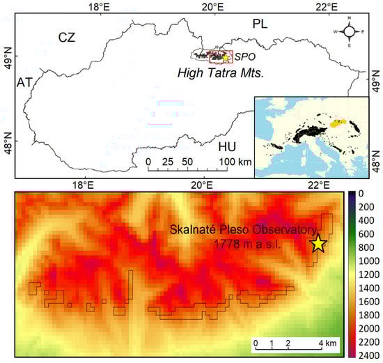
Figure 1.
The location of High Tatra Mts in Slovakia (upper). The inset shows the Pinus mugo communities in Europe and the location of Slovakia (yellow). The lower image shows the studied area with the location of the analysed pixels bounded in black lines. The yellow star marks the location of the Skalnaté Pleso Observatory (SPO) in both images.
For High Tatra Mts, a specific mountain climate with sudden to extreme weather changes is typical. The mountain massif of the High Tatras forms a natural barrier to the flow of air masses and affects the local circulation conditions and climate. Data from the SPO indicate a cool climate with a yearly air temperature that shifted from 1.7 °C (normal in 1961–1990) to 2.8 °C (normal in 1991–2020) and with annual precipitation that also increased from 1280 mm (normal in 1961–1990) to 1470 mm (normal in 1991–2020). The average annual relative air humidity varies between 68% and 80%. This locality is characterized by the frequent occurrence of mists from low clouds (mountain fog 184 days per year) supporting horizontal rainfall, mainly visible during winter in the form of icing, grey frost or increasing rainfall. The number of cloudy days with an average daily cloudiness ≥80% is 135 days per year with a high frequency during the growing season. Snowfall represents about 45% (subalpine zone) to 70% (alpine zone) of the total annual precipitation. Snow generally occurs from mid-September to mid-June, depending on the exposure and the shape of the relief. In the studied area, wind has an important role especially in storing and transporting the snow. In addition, it acts as a biometeorological element of cooling, since the heat transfer from the surface of organisms to the environment depends not only on the air temperature but also on the wind speed. The prevailing winds blow from SW (south-west). Mean wind speed varies between 2 to 8 m·s−1 depending on the direction. Over the last three decades, the frequency of occurrence of weak winds (5–20 m·s−1) as well as powerful gusty winds (50–60 m·s−1) has increased [].
2.2. Meteorological Measurements and Calculations of Winter Climate Indices
The meteorological monitoring at the SPO concentrates on examining the high mountain climate at subalpine conditions (1778 m a.s.l.). The meteorological measurements commenced in October 1940. Meteorological data represent the climate of the south slopes of this mountain region above the timberline. The observation program includes complex measurement of meteorological variables (air temperature, air humidity, atmospheric air pressure, precipitation and snow cover, wind speed and direction, components of solar radiation—global, diffused and reflected radiation, duration of sunlight, soil temperature, weather and soil conditions). These have been measured by qualified observers using the standard manual methods and measurement equipment for more than 80 years. Manual measurements are complemented by measurements using automatic weather stations. In this work, we used data on air temperature and snow cover recorded three times a day: at 7, 14 and 21 o’clock CET (Central European Time). The calibrating mercury-in-glass thermometer and maximum thermometer were the standard gauges to measure the air temperature in the standard wooden meteorological box at a height 2 m above the ground. The standard method of snow depth (SD) measurement employs a snow stake when the observers measure the SD with a precision of 1 cm. In addition, observers identify the presence of continual (more than 1 cm) or fractional snow cover, or a thin layer of sparkling snow. Measurements of SD at the current position using the snow stake started in 1978.
Winter climate indices:
- Average snow depth—ASD (cm/day) is an average of the cumulative snow depth (SDPSC) when counting for the days (dPSC) during the period of permanent snow cover (PSC).ASD = ∑SDPSC/∑dPSCThe lack of snow cover exposes the evergreen vegetation to winter desiccation and to the abrasion of sprouts by wind-blown ice. The values of winter snow depth during 2000–2020 were compared to those of the previous period, 1979–1999, to analyse changes in the snow cover.
- Winter warm spells—WWS were calculated as the incidence of five and more consecutive days when the maximum daily air temperature (TMAX) exceeded 5 °C as an interruption of the freezing period of the winter season. During this event, the increased temperature results in loss of snow cover and exposes the vegetation to initially warm and then freezing temperatures. Since the WWS can occur several times during one winter, the discrete WWS were numbered (e.g., WWS1, WWS2, etc.). To evaluate the evolution of winter warm spells, their incidence over 2000–2020 was compared to the previous periods between 1940 and 1999.
- Winter-season air temperature—TW (°C) is an average of the daily air temperatures (Td) of the winter season (W) starting on the 1st of December and ending on the 31st of March.where n is the number of days in the analysed period. The air temperature of the ith day is calculated from the term measurements at 7, 14 and 21 o’clock as defined in the following equation:TW = 1/n ∑Td,iTd,i = (T7 + T14+ 2*T21)/4Monthly air temperatures—TXII, TI, TII and TIII (°C) were calculated using the Equation (2) as averages of the daily air temperatures (Td) of December, January, February and March, respectively.
To describe the temperature conditions over the studied period:
- We applied the linear trend (Pearson’s correlation) to the average monthly air temperatures and the winter-season air temperatures over the period 1941–2020,
- We compared the average monthly air temperatures and the winter-season air temperatures to corresponding periods’ climatic normal, here known as the temperature normal (TN), calculated from the daily temperatures of 1961–1990,
- Since we have two complete climatic normal periods for SPO, 1961–1990 and 1991–2020, we analysed the differences in temperatures between the two normal periods,
- We correlated the temperatures with the average snow depth.
2.3. Vegetation Greenness from MODIS Remote Sensing Data
In this study, we employed MOD09 and MYD09 (Collection 5 and Collection 6) daily surface reflectance data products from two satellites, Terra and Aqua, with the identical spectroradiometer MODIS on-board. MOD09/MYD09 data products were radiometrically calibrated and corrected for atmospheric conditions, such as gasses, aerosols and Rayleigh scattering. The daily product was preferred to maximize the potential number of days used in evaluating the greenness of P. mugo communities. The used image data represent Earth’s spectral reflectance in a spatial resolution of 250 m (MOD09GQ and MYD09GQ product), 500 m and 1 km (MOD09GA, MYD09GA) with the level of processing 2GL. All images were obtained from the USGS archive (United State Geological Survey, http://e4ftl01.cr.usgs.gov accessed on 20 March 2021) from the period 2000–2020. The MOD09/MYD09 products contain spectral channels for NDVI calculations at a 250 m resolution—the red band 1 (RED: 620–670 nm) and the infrared band 2 (IRED: 841–876 nm). These products provide satellite data at sufficient spatial and temporal resolution for the high mountainous studied region, where a high number of cloudy and fog days typically occurs. The choice of the data products was supported by previous results, where an effect of surface anisotropy in the red and infrared band of MODIS data barely influenced NDVI estimation when obtaining Root Mean Square Error around 1% [].
The MOD09 quality analysis approach was described in our previous studies [,]. In short, at the image level, we focused on the elimination of images affected by clouds and cloud shadows as well as the impact of image distortions. From all MODIS images covering the territory of Slovakia, only cloudless or partly cloudy imagery, visually assessed at the NASA Earth Observing System Data and Information System (EOSDIS) (https://worldview.earthdata.nasa.gov/ accessed on 17 February 2021) were included in the analysis.
Another criterion for the selection of appropriate images was the satellite position in relation to the studied region during data collection. Since the MODIS tracks are stable with 16-day repetitions, we identified six images in-nadir position related to the region; four images in close-to-nadir position and six images in off-nadir position. We included in the analyses the images captured at in-nadir and close-to-nadir position. In such cases, the spatial resolution of ~250 m was achieved, and the effect of anisotropic reflectance was also reduced. As the viewing angle increases, the actual size of the acquired pixel on the Earth surface constantly changes its dimensions, extending vertically and longitudinally []. Therefore, off-nadir images were completely excluded from the analysed dataset.
In addition to the visual inspection of image quality, we analysed the quality of recorded reflectance at the pixel level using 1 km Reflectance Data State QA layer present in the MOD09GA/MYD09GA products. Each State QA pixel contains data such as whether the pixel was flagged as land, water or as containing cloud, aerosol, snow or fire (Table 1).

Table 1.
MOD09GA/MYD09GA—1 km Reflectance Data State Quality Assurance layer. Accepted combinations are indicated by values and text in bold.
The quality of individual pixels is encoded as the values of individual bits in a 16-bit integer (Table 2). We selected pixels with the following bit values: 8, 72, 76, 136, 140, 200 and 8200. Other pixel values were replaced with 0.
Table 2.
Accepted combination of DN values of the Quality Assurance flags for the product MOD09/MYD09.
After applying the criteria for image and pixel selection, NDVI values representing the vegetation greenness were then calculated over the period between 2000–2020 using the Formula (4).
NDVI = (IRED − RED)/(IRED + RED)
Pixels, where the P. mugo is mixed with other tree species, were excluded from the analyses. We worked with NDVI data of the summer season—from the beginning of August to the mid of September, when the new sprouts already appear and the clear sky condition prevails. Analysing NDVI data of this season eliminate the episodes of snowing and snow cover incidence usually present in High Tatra Mts during late spring and early autumn. The inter-annual changes of P. mugo greenness were calculated as the difference between NDVI of two consecutive summers. NDVI defines values that are expressed in hundredths from −1.0 to 1.0. The differences of NDVI would be very small values, therefore we transformed them into relative values—percentages.
2.4. Altitude and Density of Studied P. mugo Thickets
The studied area in the subalpine belt contains 153 MODIS pixels with different coverage of P. mugo at altitudes from 1500 to 2000 m a.s.l. We assumed that P. mugo growing at the same altitudes and in thickets with similar densities would respond similarly to the climate conditions.
Altitudinal zones. Altitude is a factor considerably influencing the microclimate, particularly the temperature, precipitation and wind speed conditions, in high mountains. Generally, with the increasing altitude the precipitation and wind speed increase and the temperature decreases. The altitudinal range of P. mugo communities was divided into five altitudinal zones with the step of 100 m. The lowest was altitudinal zone A1, between 1500 and 1600 m a.s.l. and the highest was altitudinal zone A5, between 1900 and 2000 m a.s.l.
Density classes. NDVI values in the studied subalpine region ranged from 0.31 to 0.88 indicating the amount of greenness in the areas with the lowest and the highest density of P. mugo shrubs, respectively (Figure 2). Firstly, averaging the pixel NDVI over the period 2000–2020, we obtained the mean amount of greenness of P. mugo per MODIS pixel. Pixels were sorted into six classes (C1–C6), each with an interval range of 0.1 (Table 3) according to their average NDVI. Next, we calculated the class averages for each year. Using the correlation matrix, we calculated Pearson´s correlation coefficients between the classes C1–C6 to reveal if there were any significant correlations between them indicating similar reactions of P. mugo to the climate conditions:
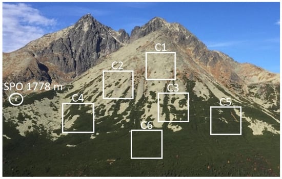
Figure 2.
The photography of the studied region near Skalnaté Pleso Observatory (SPO, 1778 m a.s.l.) illustrates the densities in the P. mugo classes (C1–C6) described in Table 3. The white squares are for illustrative purposes only and do not correspond with the MODIS pixels.
Table 3.
Classification of pixels with P. mugo into density classes based on their average NDVI values.
- The highly significant correlation (p < 0.01) was exhibited between classes C2 and C3 (R = 0.75); C4 and C5 (R = 0.72); C5 and C6 (R = 0.75).
- While C1 significantly correlated with C2 (R = 0.48) and C3 (R = 0.53), no correlation was revealed between C1 and C5 (R = 0.04) and C6 (R = 0.06), and a weak correlation was found between C1 and C4 (R = 0.30). The correlation coefficient between C3 and C4 was lower than that between C4 and C5, and C4 and C6.
- Following the correlations, we created two density classes, where pixels with lower amount of greenness indicated by NDVI between 0.31–0.60 (classes C1, C2, C3) were classified as sparse thickets (density class D1) and pixels with higher amount of greenness indicated by the NDVI between 0.61–0.90 (classes C4, C5, C6) were classified as dense thickets (density class D2) (Table 3).
The determined density classes were validated by in situ inspections using the GPS coordinates of MODIS pixels. Figure 2 illustrates the coverage of P. mugo shrubs in classes C1–C6 (Table 3) near SPO.
The changes in P. mugo greenness were evaluated separately for each altitudinal zone and density class. We applied a partial correlation analysis to analyse the relationship between winter climate indices—average snow depth (ASD), winter warm spells (WWS) and average temperatures (T), and the inter-annual differences of NDVI, controlling the effect of summer climate. In the sufficiently precipitated area, such as the subalpine belt in High Tatra Mts, the air temperature during the relatively short growing season was considered as the main climate factor able to influence the vegetation greenness. The summer temperature was calculated using Equation (2) as an average temperature of the summer months—June, July and August (TS). The partial correlation was considered significant when the correlation coefficient r exceeded the critical value rα,f, at the significance level α = 0.05.
Using ANOVA (analysis of variance), we analysed the changes in vegetation greenness between 2000 and 2020 (NDVIdif,y):
and between the average NDVI changes over five-year-long periods 2000–2004 and 2016–2020 (NDVIdif,5y):
to evaluate the significance level of changes of the greenness between density classes and altitudinal zones. Following ANOVA, we compared the mean of one group with the mean of another. We used Fisher’s Least Significant Difference (LSD) post hoc test to identify groups that significantly differ from each other.
NDVIdif,y = NDVI2020 − NDVI2000
NDVIdif,5y = NDVI2016–2020 − NDVI2000–2004
3. Results
3.1. Effect of Winter Climate Indices on P. mugo Greenness
Snow depth. Measurements of the snow depth from SPO show that the average snow depth (ASD) during the snow cover period was highly variable ranging from 13.6 cm measured in 2011 and 53.1 cm in 2007. The mean ASD for years 2000–2020 was 31.7 cm and is set as zero in Figure 3 (left). The trend indicates that the ASD decreased over the analysed period. However, as is shown in Figure 3 (right), the long-term data do not indicate a significant decreasing trend of ASD. Furthermore, the mean ASD in 2000–2020 was higher than in years 1979–1999 by 1.6 cm.
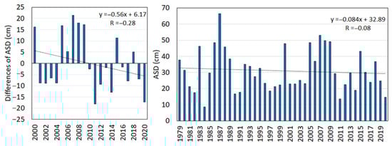
Figure 3.
The difference of average snow depth (ASD) from its average value of the period 2000–2020 (31.7 cm) indicates a decreasing trend by −0.56 cm year−1 (left), which is, however, not seen in the long-term data (−0.084 cm year−1) between 1979–2020 (right).
The results of partial correlation analyses indicated the positive inter-annual differences of NDVI when the higher ASD occurred, and negative differences of NDVI caused by the lower ASD. The negative effect of lower ASD on the P. mugo greenness was significant at lower altitudes A2 (1600–1700 m a.s.l.) (Table 4) and close to significant in the dense class D2. The P. mugo shrubs growing at higher altitudes with a height of about half a meter are better protected by snow, although lower, compared to the shrubs at lower altitudes, which grow up to 2 m. Similarly, the exposition of taller shrubs to strong winter winds is greater. Therefore, especially in years when the snow cover is low, the thin layer of snow falls through the branches of the taller shrubs to the ground. This leads to the loss of the insulation function of the snow cover protecting the aboveground parts of vegetation from the winter desiccation during freezing temperatures, photo-inhibition and from the abrasion of shoots by wind-blown ice particles. As a result, the decreased vegetation greenness after winters with the lack of snow relates with the exposure of P. mugo to the extreme weather conditions due to insufficient protection of snow layer.
Table 4.
Partial correlations between inter-annual differences of P. mugo NDVI and the winter climate indices, while controlling for the effects of summer temperature TS. The significant correlation with p < 0.05 is in bold.
Winter warm spells. According to the measurements of maximum daily air temperatures (TMAX), winter warm spells (WWS) occurred during eight winter seasons through the studied period 2000–2020. During these WWS, the daily maximum temperatures rose to above 5 °C for at least five consecutive days before returning to freezing temperatures leading to the decrease of snow depth (Table 5). Comparing the incidence of WWS in the period 2000–2020 to that recorded since the measurement started at SPO in October 1940, the frequency of years with these events increased in the last two decades. While in the period of twenty years 1941–1960 as well as 1961–1980, we recorded six years with WWS in each and during 1981–2000 only four WWS were recorded, in 2001–2020 we observed eight years with WWS (Figure 4). These historical measurement data indicate that the winter warm spells are commonly occurring winter extreme events in High Tatra Mts, however, their occurrence over the studied period 2000–2020 became more frequent.
Table 5.
The occurrence of discrete winter warm spells (WWS1, WWS2) in individual years observed during the studied period 2000–2020.
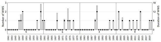
Figure 4.
Frequency (left vertical axis, diamonds) and duration (right vertical axis, bars) of winter warm spells recorded throughout the 80-year period of meteorological measurements at the Skalnaté Pleso Observatory (1941–2020).
Similar to the effect of the deficit of snow cover, the occurrence of the WWS caused the decrease of P. mugo greenness. The negative correlation between WWS and NDVI differences from the year preceding and following these events was indicated by the significant correlation coefficients in dense thickets D2 in the altitudinal zones A2 (1600–1700 m a.s.l.) and A3 (1700–1800 m a.s.l.) (Table 4). The injury of higher pine shrubs at these altitudes relates to the abrupt decrease of snow depth during the episodes with temperatures highly above freezing. Shoots protruding above the snow surface or completely exposed after snow melting suffer from the winter desiccation, photo-inhibition and abrasion by wind-blown ice particles before the fresh snow covers them repeatedly.
Temperature. The analysis of the temperature data recorded in High Tatra Mts revealed the gradual increase of all temperature indices. Over the last 80 years, the linear trends (Figure 5) indicate the increase of monthly air temperatures by:
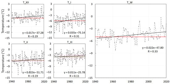
Figure 5.
Dashed lines show the average monthly air temperatures of December (T_XII), January (T_I), February (T_II) and March (T_III) and the winter-season average (T_W) from 1941 to 2020. Solid black lines mark the clear increasing trends in winter air temperatures at Skalnaté Pleso Observatory (1778 m a.s.l.). The solid red lines are corresponding temperatures of the normal period 1961–1990, providing the reference level to the current temperature increase.
- 0.17 °C per decade in December (overall 1.4 °C),
- 0.35 °C per decade in January (overall 2.8 °C),
- 0.23 °C per decade in February (overall 1.8 °C),
- 0.11 °C per decade in March (overall 0.9 °C),
- 0.22 °C per decade in the winter season (overall 1.8 °C).
Similar to the temperature increase indicated by the trends, the difference between the temperature normal (TN) of the period 1961–1990 and 1991–2020 exhibited a winter temperature increase. The highest temperature increase was recorded in January (Figure 5). January, with TN −4.5 °C in 1991–2020, became warmer than February with TN −5 °C, although in 1961–1990 TN values for both months were equal to −5.8 °C. During the last normal period 1991–2020, the March and December temperatures became equal with TN −3.3 °C, while in 1961–1990 the TN of March (−3.9 °C) was lower than the TN of December (−3.6 °C).
The growing season at high altitudes is generally short, but the warming in months at the beginning and end of the dormant period leads to its prolongation. According to the partial correlation analyses (Table 4), higher temperatures in Decembers (TXII) were beneficial for the P. mugo thickets. When controlling the effect of the summer temperatures (TS), the correlation coefficient R = 0.47 indicated significant positive effects of TXII on the increase of greenness in all P. mugo pixels in the following summer. The most pronounced effect occurred in density class D1 (R = 0.57) and in altitudinal zones A4 (R = 0.63) and A5 (R = 0.44). The warmer December indicates the later onset of winter freezing temperatures and provides more time for lignification of current year fresh shoots, which are more resistant to the extreme winter weather events. We also found a significant positive effect of warmer winter seasons on NDVI increase in the sparse P. mugo thickets (D1) with R = 0.50 and at higher altitudes A4 (R = 0.49) and A5 (R = 0.53). The mild winters resulting in the increase of P. mugo greenness at higher altitudes create advantageous conditions for thermophilisation of the alpine zone by P. mugo.
The average monthly temperatures and temperatures of the winter season were correlated to the average snow depth values, since it is reasonable to assume that the temperature affects the characteristics of snow. The analyses revealed significant correlation with the temperature of March with the R = −0.53 (Figure 6). As we previously showed in Figure 5, compared to the other winter months, the temperatures in March increased the least in 1941–2020. Comparing the TN of 1961–1990 to TN of 1991–2020, the TN in March increased by 0.6 °C. We assume that the ASD has remained balanced over the period 1980–2020 because of only the slight increase in March temperatures.
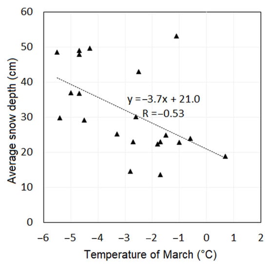
Figure 6.
Correlation between the temperatures of March and average snow depth measured at the Skalnaté Pleso Observatory (1778 m a.s.l.) in the period 2000–2020. The correlation is significant with R = −0.53 and shows a decreasing average snow depth with increasing temperature in March.
3.2. Greenness at the Beginning and End of the Studied Period 2000–2020
Analyses of inter-annual changes of vegetation greenness in density classes and altitudinal zones of P. mugo revealed the alternation of years with considerable injuries and years with expansive greening. Comparing the altitudinal zones, the overall greenness increase in 2020 compared to 2000 (NDVIdif,y) was the greatest in A5, with a slight increase in A3, close to zero in A4 and negative in A1 and A2 (Figure 7a). With respect to the density of P. mugo thickets, the increase of NDVIdif,y was observed in D1 in contrast to the decreased greenness in D2 (Figure 7b). These results are consistent with those presented in the previous chapter, since in 2020 compared to 2000, the low average snow depth led to the decrease of the NDVI in D2 and A1 and A2 while the higher temperatures affected positively the increase of greenness in D1 and in A5. The one-way ANOVA indicated significant NDVIdif,y between altitudinal zones´ means with p = 0.003 (Figure 7a) and between density classes´ means p = 0.000 (Figure 7b).
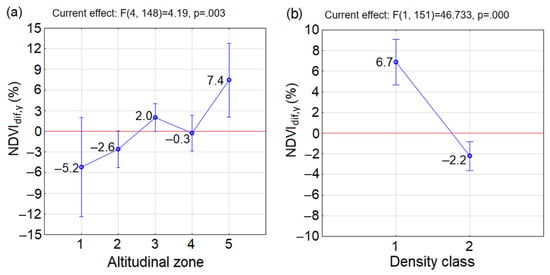
Figure 7.
Change of vegetation greenness in P. mugo thickets between 2020 and 2000 (a) in each altitudinal zone and (b) in density classes. The blue circle marks the group mean and the vertical bars denote the 0.95 confidence intervals. The positive values indicate the increase of NDVI in 2020 compared to 2000, and vice versa.
The NDVIdif,y between 2020 and 2000 was highly climate-related and was not suitable for the evaluation of the long-term changes in P. mugo communities. Therefore, we calculated the five-year NDVI averages, which are more representative than the annual NDVI and reflect the climate of a longer period. The differences of the average NDVI (NDVIdif,5y) from years at the beginning (2000–2004) and the end (2016–2020) of the studied period (Figure 8) were smaller compared to the NDVIdif,y between 2000 and 2020 (Figure 7). Comparing the altitudinal zones, the increased greenness in 2016–2020 compared to 2000–2004 was observed in zones A3 and A5 with the increment of NDVI 1.5% and 1.1%, respectively (Figure 8a). In the zones A2 and A4, the NDVIdif,5y was negative, but minor. In the zone A1, the negative NDVIdif,5y by −2.7% was revealed (Figure 8a). In regards to the density of P. mugo thickets, the increase of NDVI was small by 1.4% in the sparse density class (D1). In the dense thickets (D2), the NDVIdif,5y was negative, but again close to zero (Figure 8b). The one-way ANOVA indicated significant differences between altitudinal zones’ means with p = 0.033 (Figure 8a) and between density classes´ means p = 0.045 (Figure 6b).
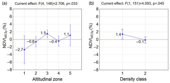
Figure 8.
Change of vegetation greenness of P. mugo between the end (2016–2020) and the beginning (2000–2004) of the studied period (a) in each altitudinal zone and (b) in density classes. The blue circle marks the group average and the vertical bars denote the 0.95 confidence intervals. The positive values indicate the increase of NDVI in 2016–2020 compared to 2000–2004 and vice versa.
Following the inconsistent results between altitudinal zones revealed using one-way ANOVA, since the NDVIdif,5y shown in Figure 8a is weighted by the number of pixels (N) in altitudinal zones and density classes, we applied the multi-factorial ANOVA to the NDVIdif,5y. The Fisher Post Hoc LSD test revealed the probability of differences between NDVIdif,5y in the combinations of pair means of altitudinal zones (A) and density classes (D). NDVIdif,5y represents the overall increase (decrease) of P. mugo greenness when the increment is positive (negative) between the end (2016–2020) and the beginning (2000–2004) of the studied period 2000–2020 under climate change. With increasing altitude, going from A1 to A5, the P. mugo thickets become less dense. This is illustrated by the number of MODIS pixels N (Table 6), e.g., NA1D1 = 0 and NA1D2 = 5, meaning that there are no sparse thickets at the lower altitude, in contrast with NA5D1 = 7 and NA5D2 = 2, which means in the highest altitudinal zone A5 there are more sparse pixels than dense. This effect of decreasing density with increasing altitude can also be seen on the slope of the mountain in Figure 2.
Table 6.
Multi-factorial ANOVA with Fisher’s Least Significant Difference (LSD) Post Hoc tests of probabilities of differences of NDVI (NDVIdif,5y) between the end (2016–2020) and the beginning (2000–2004) of the studied period between groups of altitudinal zones (A) and density classes (D). The significant differences between combinations of A and D with p < 0.05 are in bold. The positive mean NDVIdif,5y values indicate the increase of NDVI in 2016–2020 compared to 2000–2004 and vice versa.
The significant differences between combinations of A and D with p < 0.05 mean that these combinations in the groups react differently to climate change. One might expect similar responses to climate change (insignificant differences) of P. mugo between neighbouring altitudinal zones as well as opposite responses in density classes (significant differences). The results of the Fisher Post Hoc LSD test (Table 6) are listed below:
- Similar reactions of P. mugo to climate change occurred in sparse classes along altitudes (insignificant differences between combinations of D1A2, D1A3, D1A4 and D1A5). The p = 0.05 (but insignificant) between neighbouring sparse classes D1A2 and D1A3 pointed at the considerable difference between them. This may indicate, that the reaction to the climate change in sparse thickets was negative up to altitudinal zone A2, above which it became positive. This confirmed negative mean NDVIdif,5y in D1A2 and positive mean NDVIdif,5y in D1A3, D1A4 and D1A5. However, it is important to mention that only a single MODIS pixel, ND1A2 = 1, is probably not a representative sample of this group.
- In the dense class D2, significant differences occurred only between D2A3 and D2A4, while the other combinations of D2 and altitudinal zones differed insignificantly.
- Significant differences were found in combinations between different densities and altitudinal zones occurring in D2A1, D2A2 and D2A4 and D1A3. For the first three combinations the NDVIdif,5y decreased, which indicates that the changing climate influenced these dense stands negatively.
- In D1A3, the highest increase of mean NDVIdif,5y of P. mugo stands out among the other groups over the last two decades and was determined to be the most positive response to climate change. The increase of mean NDVIdif,5y under climate change was recorded also in combinations D2A3, D1A4, D1A5 and D2A5.
- Differences between D1 and D2 in individual altitudinal zones were insignificant.
Following these results, we summarized that at lower altitudes A1 and A2 with both densities and in A4 with the dense thickets, climate change induced the decrease of NDVIdif,5y. On the contrary, at both densities in higher altitudinal zones A3, A4 and A5 (except for D2A4), climate change acted positively and the greenness increased. One pair of combinations, D2A3 and D2A4, remains controversial because in these neighbouring altitudinal zones the greenness of dense class decreased in A4 while it increased in A3 (Table 6).
4. Discussion
In High Tatra Mts, P. mugo fulfils important ecosystem functions. These consist of a wide range of actions to protect soil from water and wind erosion, landslides and devastating snow avalanches, water management including the regulation and accumulation function, as well as influencing the water quality and hygiene and affecting the microclimate. Similar to the other mountain plant communities, P. mugo faces extreme environmental conditions and climate change. In this study, we present the results based on satellite data from MODIS to examine the effect of winter climate on the inter-annual variability of greenness in P. mugo thickets. Winter climate was represented by three climate indices—winter warm spells, average snow depth and average temperatures in winter.
Plants in cold environments benefit from winter snow cover, which provides thermal insulation, reduces exposure to low-temperature extremes, fluctuating temperatures [], winter desiccation and abrasion of needles and sprouts by wind-blown ice crystals [,,] and protects from photo-inhibition []. A significant factor influencing the snow depth is forest density since, in sparse forests, the snow depth is considerably greater than in dense healthy forests []. Our results show negative inter-annual changes in P. mugo greenness occurring in the dense thickets D2 (R = 0.45), which were indicated in the partial correlation analyses as close-to-significant. The decrease of greenness was most pronounced at lower altitudes in A2 (R = 0.50). P. mugo at the lower altitudes grows up to 2 m in height, therefore, especially in years when the snow cover is low during the winter, the thin layer of snow falls through the branches to the ground. This leads to the loss of the insulation function of the snow cover protecting the aboveground parts of vegetation. While the complete snow cover prevents the reduction in efficiency of photosystem II (PSII), the incomplete snow cover may lead to higher water losses as well as lower dehydration tolerance, because both osmotic adjustment and changes in turgor maintenance capacity are reduced []. The photo-inhibition of PSII is often a photo-protective strategy rather than a damaging process []. However, symptoms of low-temperature damage to the photosynthetic apparatus (e.g., degradation of leaf pigments) are particularly evident when substantial light intensity follows the exposure to low temperatures []. During low snow depth conditions, the injury of needles and branches exposed to winter desiccation during freezing temperatures together with the photo-inhibition and the abrasion of shoots by wind-blown ice particles manifested as the decrease of NDVI in the following summer. For NDVI, the damaged assimilatory organs are characterized by an increase of reflectance in the red spectral band and a decrease of the signal in the near-infrared band. The increased reflectance in the red band relates to the damage of chlorophyll in cellular structures when the absorbance of the radiation in the red spectra is reduced.
Since climate change can cause snow amount and snowpack period reduction [,] and continual shift from snow to rain in mountain regions [,], these trends in winter climate and snow cover characteristics should be taken into account when predicting climate change effects on mountain ecosystems []. A substantial decrease in snow depth (SD) and earlier snowmelt may affect plant phenology, growth and reproduction in alpine communities []. However, the snow cover trends in the mountain areas differ over the world [,,,]. Our results from High Tatra Mts (Western Carpathians) show a decreasing trend of average snow depth (ASD) over the studied period 2000–2020. However, the data over a longer period 1980–2020 point to the alteration of years with lower and higher ASD. Yet, compared to the previous period (1979–1999), the ASD of 2000–2020 was higher by 1.6 cm. Such a high decadal-scale variability but little evidence of long-term snow cover trends linked to climate warming were identified also in the mountain regions of Bulgaria (southeast Europe) []. Although we recorded the overall warming in all the winter months (TXII, TI, TII, TIII) and the whole winter season (TW) (Figure 5), the influence on the average snow depth was demonstrated only in correlation with temperatures in March (Figure 6). We assume that the long-term ASD values persist in a balanced manner since the trend in March temperatures over 1941–2020 increased only slightly (Figure 5). These results are consistent with previous findings [,,,,,,,,,,,,,], which show that the recent snowpack losses are associated with late winter warming that decreases snow accumulation while also advancing and increasing snowmelt.
In central Europe, recent air temperature increases during the winter seasons translated into an increased number of warm days. In Germany and Poland, on average of 3–5 warm spells per decade were recorded in 1966–2016, with the most numerous warm spells occurring in the second half of this period []. Our results agree with the reported increasing number of warm spells. Over the studied period 2000–2020, we recorded the highest number of years with winter warm spells (WWS) in High Tatra Mts. The occurrence of these events during winters caused negative deviations of the P. mugo greenness in the following summers. The partial correlation analyses revealed that the occurrence of WWS caused a significant decrease in the greenness of the dense thickets D2 (R = −0.47) in altitudinal zones A2 (1600–1700 m a.s.l.) and A3 (1700–1800 m a.s.l.) with R = −0.54 for both zones. The loss of snow cover occurring during the WWS exposes the assimilatory organs to wind abrasion, winter desiccation and photo-inhibition before the fresh snow covers them again. The needle desiccation and mortality are strongly affected by exposure to wind. Windward needles have lower water contents, xylem pressure potentials and viability, compared to leeward needles, while the dehydration and mortality of the needles below the snow surface are minimal []. The negative effects of winter warm spells may lead to damage in the landscape-scale-extent. Bokhorst [] concluded that WWSs in the winter of 2007/08 caused the damage of extensive areas of dwarf shrub Empetrum hermaphroditum in the sub-arctic region in Scandinavia resulting in 87% less summer growth compared to the neighbouring undamaged areas []. In addition, during winters when frozen soil blocks water uptake for several months, the low water potentials in combination with freeze–thaw events such as WWS can lead to the formation of xylem embolism []. The altitude of the timberline in High Tatra Mts ranges from 1500 to 1800 m a.s.l. depending on the stand and climate conditions, therefore not only P. mugo stands in A1 but also those in A2 and A3 neighbour with the taller trees at the timberline. Recurring injury of dense P. mugo thickets at lower altitudes (A2, A3) after the winters with the low average snow depth or winter warm spells may disadvantage this species in the competition with other mountain species utilizing the conditions of warmer climate at the timberline, such as Norway spruce (Picea abies) [,,,]. However, the acting factors such as the soil-nutrition conditions [] and toxic pollutants [,,,] may limit the competitive pressure of these taller tree species.
As mentioned earlier, the short-term temperature increases occurring as the warm spells during winter season caused injury to P. mugo in the dense thickets in the lower altitudinal zones. However, warmer winter seasons and especially December led to a significant increase of NDVI particularly in sparse P. mugo thickets at higher altitudes. These results indicate that the winter temperatures are important driving factors leading to the expansion of P. mugo greenness towards higher altitudes. Following the climate warming, represented by the temperature increase by 1.4 °C in December, 2.8 °C in January, 1.8 °C in February, 0.9 °C in March and by 1.8 °C in winter seasons over the last 80 years (Figure 5), the greenness expansion of P. mugo can further advance. At higher altitudes, the mild winter seasons will decrease the injuries caused to this evergreen conifer species by freezing temperatures in the seasons with insufficient snow depth. Depending on the temperature, the growing season at high altitudes is generally short, but the warming in months at the beginning and end of the growing season leads to its prolongation. Our results revealed that temperature increase in the first winter month—December—led to the significant increase of P. mugo greenness in the following summer (R = 0.47) in all pixels, with the most pronounced effect in the sparse P. mugo thickets (R = 0.57) at higher altitudes A4 (0.63) and A5 (R = 0.44). The later onset of winter freezing temperatures provides more time for the lignification of current year fresh shoots and thus enhances their resistance to extreme winter weather events.
Across the studied subalpine area in High Tatra Mts, we found a considerable effect of stand factors—altitude and density, on the NDVIdif,5y between the beginning (2000–2004) and end (2016–2020) of the studied period. At lower altitudes—A1 and A2—with both densities and in A4 with the dense thickets, climate change induced the decrease of NDVIdif,5y. On the contrary, at both densities in higher altitudinal zones A3, A4 and A5 (except for D2A4), climate change acted positively and the greenness increased. It is important to emphasize that the density in D2 at higher altitudes (A3–A5) does not exclusively constitute totally closed canopies, but also includes the areas of P. mugo interrupted by rocky fields (Table 3, Figure 2). Here, the increase of greenness via the growth expansion under favourable climate conditions is still possible. Previous studies using ortophoto maps documented rapid expansion of P. mugo into alpine meadows [,,]. The fastest expansion occurred within open stands [] with short pine polycormon margins []. In favourable conditions, P. mugo with its branching growth is able to cover the ground to a degree that excludes most other vegetation (except shade tolerant mosses) within a span of few decades []. Therefore, expanding P. mugo thickets can exert a strong negative influence on the biodiversity of alpine meadows by reducing the habitat of heliophytic alpine plants and many insect species []. The favourable climate conditions relating to climate warming support the thermophilisation of high mountain areas by vital P. mugo shrubs suppressing the valuable alpine ecosystems and endemics. Recent research in mountain summits in Europe indicated gradual decrease of cold-adapted alpine species [,] and warming-related colonization of subalpine vascular species, particularly shrubs, into alpine summits. On the south-facing slopes analysed in this study, the colonization is expected to be more pronounced [].
5. Conclusions
In the preservation of all ecosystems against the climate change, the monitoring of climate impacts is a priority. With the continual increase of winter temperatures, any damage to vegetation may incur major consequences for the biodiversity of the subalpine and alpine ecosystems. In the presented study, we selected the main winter climate indices using the temperature and snow cover data to analyse the impacts of climate change and winter weather conditions on the P. mugo thickets in the subalpine area of High Tatra Mts (Western Carpathians). We employed remote sensing NDVI data to quantify the inter-annual changes of this evergreen conifer. The landscape observations of P. mugo provided compelling evidence that winter climate indices can explain the inter-annual variations of greenness.
Our main results are as follows:
- Across the studied subalpine area in High Tatra Mts, we found a considerable effect of stand factors—altitude and density, on the changes of P. mugo greenness induced by the winter climate.
- We observed a negative effect of winter warm spells in dense P. mugo thickets and at lower altitudes, because the warmer weather melts the snow cover, which serves as the protection to abrasion of needles and sprouts by windblown ice, winter desiccation and photo-inhibition.
- A positive correlation was found between greenness and average snow cover depth in dense thickets, indicating that the P. mugo benefits from the protection of higher snow cover. However, after winters with low snow cover, when the protection was insufficient, P. mugo greenness decreased in the following summer.
- We also found a positive effect of the rising winter temperatures on the greenness of sparse thickets in the following summer, which we interpret as mild winters having a less deteriorating effect on the greenness of P. mugo.
- Our results revealed that the temperature increase in the first winter month—December—caused a significant increase in the greenness of P. mugo in the following summer, particularly in sparse thickets and at higher altitudes. The later onset of winter freezing temperatures provides more time for the lignification of current year fresh shoots and thus enhances their resistance to extreme winter weather events.
- In the studied period 2000–2020, we found an overall increase of greenness at the end of the period compared to its beginning, meaning that climate warming created suitable conditions for P. mugo and advanced its expansion into the alpine zone.
Expansion of species into new territories has the potential to cause adverse changes to the ecosystems. At the higher altitudes (1800–2000 m a.s.l.), we expect that further warming of winter seasons will decrease the overall injuries caused to P. mugo by freezing temperatures in the seasons with a snow cover deficit. This may lead to the enhancement of the thermophilisation of alpine areas by these vital shrubs, suppressing the other valuable alpine ecosystems and endemics, especially cold-adopted species. On the other hand, recurring injury of P. mugo thickets at the timberline after the winters with low snow depth or winter warm spells may disadvantage this species in the competition with other mountain species utilizing the conditions of a warmer climate. In future work, we will carry out the analyses of the combined effects of the changing climate and the oxidative stress on high mountain species near and above the timberline.
Author Contributions
Conceptualization, V.L. and Ľ.M.; methodology, V.L. and S.B.; software, T.B. and S.B.; formal analysis, S.B.; investigation, V.L., A.B., S.B.; resources, V.L.; data curation, T.B. and S.B.; writing—original draft preparation, V.L., Ľ.M; writing—review and editing, V.L., S.B., T.B., Ľ.M., A.B; visualization, V.L., Ľ.M; project administration, V.L.; funding acquisition, V.L. All authors have read and agreed to the published version of the manuscript
Funding
This research was funded by research grants of The Ministry of Education, Science, Research and Sport of the Slovak Republic: VEGA 2/0093/21.
Institutional Review Board Statement
Not applicable.
Informed Consent Statement
Not applicable.
Data Availability Statement
MODIS images—NASA Earth Observing System Data and Information System (EOSDIS): https://worldview.earthdata.nasa.gov/ accessed on 17 February 2021. MOD09/MYD09 collection 5: https://patarnott.com/satsens/pdf/MOD09_UserGuide_v1_2.pdf (accessed on 17 February 2021). MOD09/MYD09 collection 6: https://modis-land.gsfc.nasa.gov/pdf/MOD09_UserGuide_v1.4.pdf (accessed on 17 February 2021).
Acknowledgments
Veronika Lukasová acknowledges support from the Stefan Schwarz fund for postdoctoral researchers awarded by the Slovak Academy of Sciences. In addition, the authors are very grateful to all members of the technical staff from the Department of Atmospheric Physics (ESI SAS), and from the Slovak Hydro-Meteorological Institute for the data measured at the Skalnaté Pleso Observatory. We thank Peter Zelina for comments on an early version of the manuscript.
Conflicts of Interest
The authors declare no conflict of interest.
References
- Inouye, D.W.; Wielgolaski, F.E. Phenology of High-Altitude Climates; Schwartz, M.D., Ed.; Phenology: An Integrative Environmental Science; Kluwer Academic Publishers: Alphen, The Netherlands, 2003; pp. 195–214. [Google Scholar]
- Weiss, D.J.; Walsh, S.J. Remote Sensing of Mountain Environments. Geogr. Compass 2008, 3, 1–21. [Google Scholar] [CrossRef]
- Richardson, D.M. Ecology and Biogeography of Pinus; Cambridge University Press: Cambridge, UK, 1998; p. 527. [Google Scholar]
- Šibík, J.; Šibíková, I.; Kliment, J. The subalpine Pinus mugo-communities of the Carpathians with a European perspective. Phytocoenologia 2010, 40, 155–188. [Google Scholar] [CrossRef]
- Körner, C. Alpine Plant Life. Functional Plant Ecology of High Mountain Ecosystems, 2nd ed.; Springer: Berlin/Heidelberg, Germany; New York, NY, USA, 2003; p. 344. ISBN 978-3-642-18970-8. [Google Scholar]
- Říha, V. Jihočeské rašeliny, jejich vztah k lesu a okolí [South Bohemian peatlands, their relation to the forest and its surroundings]. Sborn. Masaryk. Akad. Práce 1938, 12, 143–194. [Google Scholar]
- Solař, J.; Janiga, M. Long-term Changes in Dwarf Pine (Pinus mugo) Cover in the High Tatra Mountains, Slovakia. Mt. Res. Dev. 2013, 33, 51–62. [Google Scholar] [CrossRef]
- Wild, J.; Winkler, E. Krummholz and grassland coexistence above the forest-line in the Krkonoše Mountains: Grid-based model of shrub dynamics. Ecol. Model. 2008, 213, 293–307. [Google Scholar] [CrossRef]
- Treml, V.; Wild, J.; Chuman, T.; Potůčková, M. Assessing the Change in Cover of Non-Indigenous Dwarf-Pine Using Aerial Photographs, a Case Study from the Hrubý Jeseník Mts., the Sudetes. J. Landsc. Ecol. 2010, 3, 90–104. [Google Scholar] [CrossRef][Green Version]
- Barry, R.G. Mountain Weather and Climate Third Edition; Cambridge University Press (CUP): Cambridge, UK, 2008; p. 506. [Google Scholar]
- Marty, C.; Meister, R. Long-term snow and weather observations at Weissfluhjoch and its relation to other high-altitude observatories in the Alps. Theor. Appl. Clim. 2012, 110, 573–583. [Google Scholar] [CrossRef]
- Wang, Q.; Fan, X.; Wang, M. Evidence of high-elevation amplification versus Arctic amplification. Sci. Rep. 2016, 6, 19219. [Google Scholar] [CrossRef]
- Ohmura, A. Enhanced temperature variability in high-altitude climate change. Theor. Appl. Clim. 2012, 110, 499–508. [Google Scholar] [CrossRef]
- Mountain Research Initiative EDW Working Group; Pepin, N.; Bradley, R.S.; Diaz, H.F.; Baraer, M.; Caceres, E.B.; Forsythe, N.; Fowler, H.; Greenwood, G.; Hashmi, M.Z.; et al. Elevation-dependent warming in mountain regions of the world. Nat. Clim. Chang. 2015, 5, 424–430. [Google Scholar] [CrossRef]
- Steger, C.; Kotlarski, S.; Jonas, T.; Schär, C. Alpine snow cover in a changing climate: A regional climate model perspective. Clim. Dyn. 2012, 41, 735–754. [Google Scholar] [CrossRef]
- Jiménez Cisneros, B.E.; Oki, T.; Arnell, N.W.; Benito, G.; Cogley, J.G.; Döll, P.; Jiang, T.; Mwakalila, S.S. Freshwater Resources, In Climate Change: Impacts, Adaptation, and Vulnerability. Part A: Global and Sectoral Aspects. Contribution of Working Group II to the Fifth Assessment Report of the Intergovernmental Panel on Climate Change; Field, C.B., Barros, V.R., Dokken, D.J., Mach, K.J., Eds.; Cambridge University Press: Cambridge, UK, 2014; pp. 229–269. [Google Scholar]
- Räisänen, J. Warmer climate: Less or more snow? Clim. Dyn. 2008, 30, 307–319. [Google Scholar] [CrossRef]
- DeMaria, E.M.C.; Roundy, J.K.; Wi, S.; Palmer, R.N. The Effects of Climate Change on Seasonal Snowpack and the Hydrology of the Northeastern and Upper Midwest United States. J. Clim. 2016, 29, 6527–6541. [Google Scholar] [CrossRef]
- Croce, P.; Formichi, P.; Landi, F.; Mercogliano, P.; Bucchignani, E.; Dosio, A.; Dimova, S. The snow load in Europe and the climate change. Clim. Risk Manag. 2018, 20, 138–154. [Google Scholar] [CrossRef]
- Räisänen, J.; Eklund, J. 21st Century changes in snow climate in Northern Europe: A high-resolution view from ENSEMBLES regional climate models. Clim. Dyn. 2012, 38, 2575–2591. [Google Scholar] [CrossRef]
- Stolina, M. Ochrana Lesa (Forest Protection); Priroda: Bratislava, Slovakia, 1985; p. 473. [Google Scholar]
- Sonesson, M.; Callaghan, T.V. Strategies of survival in plants of the Fennoscandian Arctic. Arctic 1991, 44, 95–105. [Google Scholar] [CrossRef]
- Kershaw, G.P.; Jones, H.G.; Pomeroy, J.W.; Walker, D.A.; Hoham, R.W. Snow Ecology: An Interdisciplinary Examination of Snow-Covered Ecosystems. Arctic Antarct. Alp. Res. 2002, 34, 486. [Google Scholar] [CrossRef]
- Bokhorst, S.F.; Bjerke, J.W.; Tømmervik, H.; Callaghan, T.V.; Phoenix, G.K. Winter warming events damage sub-Arctic vegetation: Consistent evidence from an experimental manipulation and a natural event. J. Ecol. 2009, 97, 1408–1415. [Google Scholar] [CrossRef]
- Tomczyk, A.M.; Sulikowska, A.; Bednorz, E.; Półrolniczak, M. Atmospheric circulation conditions during winter warm spells in Central Europe. Nat. Hazards 2019, 96, 1413–1428. [Google Scholar] [CrossRef]
- Gottfried, M.; Pauli, H.; Futschik, A.; Akhalkatsi, M.; Barančok, P.; Alonso, J.L.B.; Coldea, G.; Dick, J.; Erschbamer, B.; Calzado, M.R.F.; et al. Continent-wide response of mountain vegetation to climate change. Nat. Clim. Chang. 2012, 2, 111–115. [Google Scholar] [CrossRef]
- Kopáček, J.; Kaňa, J.; Bičárová, S.; Brahney, J.; Navrátil, T.; Norton, S.A.; Porcal, P.; Stuchlík, E. Climate change accelerates recovery of the Tatra Mountain lakes from acidification and increases their nutrient and chlorophyll a concentrations. Aquat. Sci. 2019, 81, 70. [Google Scholar] [CrossRef]
- Kerr, J.T.; Ostrovsky, M. From space to species: Ecological applications for remote sensing. Trends Ecol. Evol. 2003, 18, 299–305. [Google Scholar] [CrossRef]
- Beck, P.S.; Atzberger, C.; Høgda, K.A.; Johansen, B.; Skidmore, A.K. Improved monitoring of vegetation dynamics at very high latitudes: A new method using MODIS NDVI. Remote Sens. Environ. 2006, 100, 321–334. [Google Scholar] [CrossRef]
- Dunn, A.H.; De Beurs, K.M. Land surface phenology of North American mountain environments using moderate resolution imaging spectroradiometer data. Remote Sens. Environ. 2011, 115, 1220–1233. [Google Scholar] [CrossRef]
- Hmimina, G.; Dufrêne, E.; Pontailler, J.-Y.; Delpierre, N.; Aubinet, M.; Caquet, B.; De Grandcourt, A.; Burban, B.; Flechard, C.R.; Granier, A.; et al. Evaluation of the potential of MODIS satellite data to predict vegetation phenology in different biomes: An investigation using ground-based NDVI measurements. Remote Sens. Environ. 2013, 132, 145–158. [Google Scholar] [CrossRef]
- Bucha, T.; Koreň, M. Phenology of the beech forests in the Western Carpathians from MODIS for 2000 2015. iForest Biogeosci. For. 2017, 10, 537–546. [Google Scholar] [CrossRef]
- Lukasová, V.; Bucha, T.; Škvareninová, J.; Škvarenina, J. Validation and Application of European Beech Phenological Metrics Derived from MODIS Data along an Altitudinal Gradient. Forests 2019, 10, 60. [Google Scholar] [CrossRef]
- Dai, L.; Palombo, C.; Van Gils, H.; Rossiter, D.G.; Tognetti, R.; Luo, G. Pinus mugoKrummholz Dynamics During Concomitant Change in Pastoralism and Climate in the Central Apennines. Mt. Res. Dev. 2017, 37, 75–86. [Google Scholar] [CrossRef]
- Minďáš, J.; Lapin, M.; Škvarenina, J. Climate Change and Forest in Slovakia (in Slovak). Národný Klimatický Program SR (National Climate Program SR); MŽP SR: Bratislava, Slovakia, 1996; Volume 5, p. 96. [Google Scholar]
- Škvarenina, J.; Križová, E.; Tomlain, J. Impact of the climate change on the water balance of altitudinal vegetation stages in Slovakia. Ekológia 2004, 23, 13–29. [Google Scholar]
- Ďurský, J.; Škvarenina, J.; Minďáš, J.; Mikova, A. Regional analysis of climate change impact on Norway spruce (Picea abies L. Karst.) growth in Slovak mountain forests. J. For. Sci. 2012, 52, 306–315. [Google Scholar] [CrossRef]
- Bičárová, S.; Bezák, V.; Bilčík, D.; Čepčeková, E.; Fleischer, P.; Hlavatá, H.; Holko, L.; Jakubják, O.; Mačutek, J.; Majcin, D.; et al. Observatory of SAS at Skalnaté Pleso-70 Years of Meteorological Measurements; Geophysical Institute SAS: Stará Lesná, Slovakia, 2013; p. 63. ISBN 978-80-85754-29-2. [Google Scholar]
- Franch, B.; Vermote, E.; Sobrino, J.; Fédèle, E. Analysis of directional effects on atmospheric correction. Remote Sens. Environ. 2013, 128, 276–288. [Google Scholar] [CrossRef]
- Kristof, D.; Pataki, R. Novel vector-based pre-processing of MODIS data. In Ebook Remote Sensing for a Changing Europe; IOS Press: Amsterdam, The Netherlands, 2009; pp. 483–490. [Google Scholar]
- Marchand, P.J. The Changing Snowpack. Life in the Cold, 3rd ed.; University Press of New England: Hanover, UK, 1996; pp. 11–39. [Google Scholar]
- Neuner, G.; Ambach, D.; Aichner, K. Impact of snow cover on photoinhibition and winter desiccation in evergreen Rhododendron ferrugineum leaves during subalpine winter. Tree Physiol. 1999, 19, 725–732. [Google Scholar] [CrossRef] [PubMed]
- Bartík, M.; Holko, L.; Jančo, M.; Škvarenina, J.; Danko, M.; Kostka, Z. Influence of Mountain Spruce Forest Dieback on Snow Accumulation and Melt. J. Hydrol. Hydromech. 2019, 67, 59–69. [Google Scholar] [CrossRef]
- Choudhury, N.; Behera, R. Photoinhibition of Photosynthesis: Role of Carotenoids in Photoprotection of Chloroplast Constituents. Photosynthetica 2001, 39, 481–488. [Google Scholar] [CrossRef]
- Goh, C.-H.; Ko, S.-M.; Koh, S.; Kim, Y.-J.; Bae, H.-J. Photosynthesis and Environments: Photoinhibition and Repair Mechanisms in Plants. J. Plant Biol. 2011, 55, 93–101. [Google Scholar] [CrossRef]
- Wipf, S.; Stoeckli, V.; Bebi, P. Winter climate change in alpine tundra: Plant responses to changes in snow depth and snowmelt timing. Clim. Chang. 2009, 94, 105–121. [Google Scholar] [CrossRef]
- Kirkpatrick, J.B.; Nunez, M.; Bridle, K.L.; Parry, J.; Gibson, N. Causes and consequences of variation in snow incidence on the high mountains of Tasmania, 1983–2013. Aust. J. Bot. 2017, 65, 214. [Google Scholar] [CrossRef]
- Laternser, M.; Schneebeli, M. Long-term snow climate trends of the Swiss Alps (1931–99). Int. J. Clim. 2003, 23, 733–750. [Google Scholar] [CrossRef]
- Scherrer, S.C.; Appenzeller, C.; Laternser, M. Trends in Swiss Alpine snow days: The role of local- and large-scale climate variability. Geophys. Res. Lett. 2004, 31, 31. [Google Scholar] [CrossRef]
- Brown, R.D.; Petkova, N. Snow cover variability in Bulgarian mountainous regions, 1931–2000. Int. J. Clim. 2007, 27, 1215–1229. [Google Scholar] [CrossRef]
- Kapnick, S.; Hall, A. Causes of recent changes in western North American snowpack. Clim. Dyn. 2011, 38, 1885–1899. [Google Scholar] [CrossRef]
- McCabe, G.J.; Wolock, D.M. Long-term variability in Northern Hemisphere snow cover and associations with warmer winters. Clim. Chang. 2009, 99, 141–153. [Google Scholar] [CrossRef]
- Minder, J.R. The Sensitivity of Mountain Snowpack Accumulation to Climate Warming. J. Clim. 2010, 23, 2634–2650. [Google Scholar] [CrossRef]
- Pedersen, S.H.; Liston, G.E.; Tamstorf, M.P.; Westergaard-Nielsen, A.; Schmidt, N.M. Quantifying Episodic Snowmelt Events in Arctic Ecosystems. Ecosystems 2015, 18, 839–856. [Google Scholar] [CrossRef]
- Hadley, J.L.; Smith, W.K. Influence of Wind Exposure on Needle Desiccation and Mortality for Timberline Conifers in Wyoming, U.S.A. Arctic Alp. Res. 1983, 15, 127–135. [Google Scholar] [CrossRef]
- Mayr, S.; Schmid, P.; Rosner, S. Winter Embolism and Recovery in the Conifer Shrub Pinus mugo L. Forests 2019, 10, 941. [Google Scholar] [CrossRef]
- Kromka, M. Influence of Expected Climatic Changes on Mineralization of Soil Organic Matter (in Slovak); Národný klimatický program SR (National Climate Program SR); MŽP SR: Bratislava, Slovakia, 2001; Volume 11, pp. 88–102. [Google Scholar]
- Hůnová, I.; Novotný, R.; Uhlířová, H.; Vráblík, T.; Horálek, J.; Lomský, B.; Šrámek, V. The impact of ambient ozone on mountain spruce forests in the Czech Republic as indicated by malondialdehyde. Environ. Pollut. 2010, 158, 2393–2401. [Google Scholar] [CrossRef] [PubMed]
- Sicard, P.; Dalstein-Richier, L.; Vas, N. Annual and seasonal trends of ambient ozone concentration and its impact on forest vegetation in Mercantour National Park (South-eastern France) over the 2000–2008 period. Environ. Pollut. 2011, 159, 351–362. [Google Scholar] [CrossRef] [PubMed]
- Feng, Z.; Büker, P.; Pleijel, H.; Emberson, L.; Karlsson, P.E.; Uddling, J. A unifying explanation for variation in ozone sensitivity among woody plants. Glob. Chang. Biol. 2017, 24, 78–84. [Google Scholar] [CrossRef]
- Bičárová, S.; Shashikumar, A.; Dalstein-Richier, L.; Lukasová, V.; Adamčíková, K.; Pavlendová, H.; Sitková, Z.; Buchholcerová, A.; Bilčík, D. The response of Pinus species to ozone uptake in different climate regions of Europe. Cent. Eur. For. J. 2020, 66, 255–268. [Google Scholar] [CrossRef]
- Parobeková, Z.; Bugala, M.; Kardoš, M.; Dovciak, M.; Lukáčik, I.; Saniga, M. Long-Term Changes in Dwarf Pine (Pinus mugo Turra) Cover and Growth in the Orava Beskid Mountains, Slovakia. Mt. Res. Dev. 2018, 38, 342–353. [Google Scholar] [CrossRef]
- Jørgensen, H. NOBANIS–Invasive Alien Species Fact Sheet–Pinus Mugo. Online Database of the European Network on Invasive Alien Species–NOBANIS 2010. Available online: https://www.nobanis.org/globalassets/speciesinfo/p/pinus-mugo/pinus_mugo.pdf (accessed on 19 March 2020).
- Kuras, T.; Beneš, J.; Konvička, M. Behaviour and within-habitat distribution of adult Erebia sudetica sudetica, endemic of the Hruby Jeseník Mts., Czech Republic (Nymphalidae, Satyrinae). Nota Lepidopterol. 2001, 24, 69–83. [Google Scholar]
- Pauli, H.; Gottfried, M.; Dullinger, S.; Abdaladze, O.; Akhalkatsi, M.; Alonso, J.L.B.; Coldea, G.; Dick, J.; Erschbamer, B.; Calzado, R.F.; et al. Recent Plant Diversity Changes on Europe’s Mountain Summits. Science 2012, 336, 353–355. [Google Scholar] [CrossRef] [PubMed]
- Steinbauer, M.J.; Grytnes, J.-A.; Jurasinski, G.; Kulonen, A.; Lenoir, J.; Pauli, H.; Rixen, C.; Winkler, M.; Bardy-Durchhalter, M.; Barni, E.; et al. Accelerated increase in plant species richness on mountain summits is linked to warming. Nature 2018, 556, 231–234. [Google Scholar] [CrossRef]
- Winkler, M.; Lamprecht, A.; Steinbauer, K.; Hülber, K.; Theurillat, J.-P.; Breiner, F.; Choler, P.; Ertl, S.; Girón, A.G.; Rossi, G.; et al. The rich sides of mountain summits—A pan-European view on aspect preferences of alpine plants. J. Biogeogr. 2016, 43, 2261–2273. [Google Scholar] [CrossRef]
Publisher’s Note: MDPI stays neutral with regard to jurisdictional claims in published maps and institutional affiliations. |
© 2021 by the authors. Licensee MDPI, Basel, Switzerland. This article is an open access article distributed under the terms and conditions of the Creative Commons Attribution (CC BY) license (https://creativecommons.org/licenses/by/4.0/).