Article

Integration of Visible and Thermal Imagery with an Artificial Neural Network Approach for Robust Forecasting of Canopy Water Content in Rice

1
College of Biosystems Engineering and Food Science, Zhejiang University, Hangzhou 310058, China
2
Key Laboratory of Spectroscopy Sensing, Ministry of Agriculture, Hangzhou 310058, China
3
Agricultural Engineering Department, Faculty of Agriculture, Mansoura University, Mansoura 35516, Egypt
*
Author to whom correspondence should be addressed.
Remote Sens. 2021, 13(9), 1785; https://doi.org/10.3390/rs13091785
Submission received: 29 March 2021 / Revised: 20 April 2021 / Accepted: 1 May 2021 / Published: 3 May 2021
(This article belongs to the Section Remote Sensing Image Processing)

Abstract

:
A total of 120 rice plant samples were scanned by visible and thermal proximal sensing systems under different water stress levels to evaluate the canopy water content (CWC). The oven-drying method was employed for assessing the canopy’s water state. This CWC is of great importance for irrigation management decisions. The proposed framework is to integrate visible and thermal imaging data using an artificial neural network as a valuable promising implement for accurately estimating the water content of the plant. The RGB-based features included 20 color vegetation indices (VI) and 6 gray level co-occurrence matrix-based texture features (GLCMF). The thermal imaging features were two thermal indicators (T), namely normalized relative canopy temperature (NRCT) and the crop water stress index (CWSI), that were deliberated by plant temperatures. These features were applied with a back-propagation neural network (BPNN) for training the samples with minimal loss on a cross-validation set. Model behavior was affected by filtering high-level features and optimizing hyperparameters of the model. The results indicated that feature-based modeling from both visible and thermal images achieved better performance than features from the individual visible or thermal image. The supreme prediction variables were 21 features: 14VI, 5GLCMF, and 2T. The fusion of color–texture–thermal features greatly improved the precision of water content evaluation (99.40%). Its determination coefficient (R2 = 0.983) was the most satisfied with an RMSE of 0.599. Overall, the methodology of this work can support decision makers and water managers to take effective and timely actions and achieve agricultural water sustainability.

1. Introduction

About 70–90% of global water resources are consumed through agriculture [1]. Extreme water use in the agricultural sector also causes water scarcity in semi-arid and arid regions [2]. Rice is one of the most economical crops that requires large amounts of water. Decreasing water availability for agriculture threatens the productivity of the irrigated rice ecosystem and ways to save water and increase the water productivity of rice must be found [3]. By optimizing the timing, duration, and amount of irrigation and drainage, water-saving irrigation practice has been proven effective in saving water and increasing rice yield [4]. To improve the water use efficiency of plants, it is important to accurately and timely predict crop water status. Canopy water content (CWC) is a significant factor in regard to the water use efficiency of plants [5], drought assessment [6], a key input variable in irrigation management decisions, and crop ripening monitoring [7]. Moreover, it is a vital parameter that reflects plant physiological status and health [8]. It is one of the indicators widely used to evaluate a plant’s water condition [9]. Traditionally, there are various manners of observing the water state in a plant such as lab-based leaf water content analysis [10], stomatal conductance [11], and sap flow measurement [12]. Despite the high precision delivered by these ways, they are time consuming, destructive and laborious, particularly in large-scale areas [13]. Moreover, the interest in monitoring the plant water status has increased in the scientific community through remote sensing, which is very widely used to reliably retrieve leaf water content [8].
We focused on modern procedures for estimation of the CWC from optical remote sensing data, especially from visible (RGB: red–green–blue) and thermal imaging. These have several benefits compared to hyperspectral sensors. Thermal sensing is useful since it is cheap, non-destructive, convenient, and can be done remotely [14]. Digital imaging may provide a low-cost and easy-to-use alternative [15]. The hyperspectral camera is heavy, expensive, and requires professional imaging and data processing [16]. The superiority of proximity sensing technology with regression algorithm relies on three major aspects: hand-crafted feature selection, data fusion for different sensors, and selecting the best model hyperparameters. Elsherbiny et al. [17] explained that the regression algorithms could be upgraded for robust prediction of rice water status through some actions, including high-level features nominating, hyperparameters optimization, providing various alternatives for the most sensitive features, and integrating the model with the best-combined features. Primary, common methods for extracting RGB-based features include color vegetation indices (VI) and gray level co-occurrence matrix-established texture features (GLCMF). Several studies have found that the crop water deficit will directly affect the biochemical processes and morphology of crops, and this effect can be observed in the color changes of the crop leaves. Digital images are composited by pixels, which are a combination of the color channels RGB. The VI can be calculated from these channels [18]. Wang et al. [19] generated regression models using the G–R parameter of the RGB color system with the moisture content of cotton and the moisture content index. The prediction accuracies were up to 90.7% and 91.0%, respectively. Zakaluk and Sri [20] checked the use of artificial neural networks (ANN) for digital images, taken by a 5 megapixel RGB camera to predict the leaf water potential of potato plants. Then, the relationship between leaf water potential and image features was determined.
Another variant of GLCMF was derived from RGB images to estimate the water situation in plants. Wenting et al. [21] concluded the relationship between GLCMF of the RGB image of crop leaves and leaf water content at heading-stage maize with an expected R2 value of 0.702 and the RMSE was within ±2%. Shao et al. [22] indicated that GLCMF-based partial least square regression model can predict water content in grapevines with better performance. The prediction R2 was 0.833 with an RMSE of 1.049. Additionally, the thermal imaging system can provide an indication of the water condition in the plant. Leaf temperature is an alternative measure that is a suitable indicator of a plant’s water state [23]. Moller et al. [24] showed that thermal imagery can be used to accurately estimate crop water status. Ballester et al. [25] used a handheld infrared thermal imager to study leaf moisture content in citrus trees and persimmon trees.
The integration of different data sources was a vital component of this work to improve the quality and robustness of the CWC prediction model. This has previously been used to evaluate plant phenotypes. Moller et al. [24] elucidated that the fusion of visible and thermal imaging could develop the accuracy of the crop water stress index (CWSI) computation and provide accurate data on the crop water status of grapevines. Shao et al. [22] clarified that the incorporation of both GLCMF and reflectance features could enable the prediction of water content of grapevines and be beneficial for grapevine management and achieved prediction R2 of 0.900 with an RMSE of 0.826.
The hyperparameter optimization of the model is another factor that has a significant impact on the efficiency of water content prediction. The performance of any machine learning (ML) model is profoundly affected by hyperparameter selection, which has several benefits: it can improve the performance of ML algorithms [26] and improve the reproducibility and fairness of scientific studies [27]. Furthermore, it could perform a major role in improving the prediction model because of the direct control of the behaviors of training algorithms [28]. In this research, the ANN building possibility was used as a tool to support accurate irrigation management decision making by means of visible and thermal sensors. Dawson et al. [29] developed an ANN model for predicting water content in leaves depending on single leaf reflectance and transmittance, which are important input variables to vegetation canopy reflectance models. The R2 was defined as 0.86 with an RMSE of 1.3%. Marti et al. [30] described the application of ANN to estimate stem water potential from soil moisture at different depths and standard meteorological variables, such as temperature, relative humidity, and solar radiation. The ANN presented high-performance accuracy with an optimum R2 of 0.926.
To maximize irrigation in rice fields, the plant’s water content should be explored accurately via proximal sensing systems. Although visible and thermal imagery are widely used to estimate water content in plants, the best performing algorithm has a high priority in research interests. Based on our knowledge, no prior research has implemented the hybrid methodology of BPNN with features extracted from thermal and RGB imaging to develop a predictive model for accurate estimation of the water content status of rice under different irrigation water treatments and climate change. Hence, the main objectives of this study were (i) to create a well-structured CWC modeling of rice relying on high-level features derived from RGB and thermal images, (ii) to define the superior variants of thermal and RGB features for robust CWC prediction, and (iii) to evaluate the performance of BPNN models using the best-combined features and to adopt the finest model that could be recommended for precision irrigation in the future.

2. Materials and Methods

2.1. Experimental Design

The experiment was conducted on 120 potted plants of rice under natural conditions at Zhejiang University (120°09′E, 30°14′N), Hangzhou City, Zhejiang Province, P.R. China. Often, a plastic cover was set up over the plants during precipitation to control the water added for them, and to obtain the heterogeneous water condition from the tested leaves. To prepare the germination, the rice seeds (Xiushui 134) were submerged in the water for four days at a temperature of 28–30 °C, and the water was replaced twice a day. Then, the 10 rice plants were sown into a single PVC (polyvinyl chloride) pot, which had dimensions of 140 × 95 × 125 mm. Each pot was filled with 300 g of black peat moss (HAWITA Gruppe GmbH, Germany) and was irrigated to achieve saturation during the first growing month. The compound fertilizer treatment, N–P2O5–K2O (15-15-15), with a rate of 100 kg ha−1 was applied at 10-day intervals, produced by Qingdao SONEF Chemical Company. Potted rice plants were transplanted on July 10, 2018 and divided into 3 groups, each with 40 pots. It was harvested on August 12, August 30, and September 21, 2018 for the 1st, 2nd, and 3rd groups, respectively. Table 1 shows the summary statistics of air temperature, relative humidity, and vapor pressure deficit (VPD). The values of VPD were determined from the formula stated by Abtew and Melesse [31]. In this work, there were three different growth stages of the rice plants: tillering, stem elongation, and panicle initiation. The water deficit was implemented within a period of 27–34 days, 34–52 days, and 52–74 days of plant life for the 1st, 2nd, and 3rd groups, respectively. As declared in Figure 1, an experiment was carried out with a completely randomized block design in a factorial experiment. The experimental design was divided into three groups, each comprising four irrigation treatments: fully-irrigated (T1: 100%), mild (T2: 80–70%), moderate (T3: 60–50%), and severe water stress (T4: 40–30% field capacity), respectively. The number of replicates (R1, R2, etc.) of treatment was 10 samples. Generally, the gravimetric approach was used to measure the volume of water by manually weighing pots twice a day, supplemented by replacing the transpiration of water to preserve the respective moisture stress conditions. Gross water applied volumes were estimated for each group, 1st stage values were 44.35, 41.65, 39.4, and 37.15 L (liter) for well-controlled, mild, moderate, and severe stress conditions, respectively. Their corresponding values at the 2nd group were 60.35, 56.40, 53.29, and 49.25 L and at the 3rd group were 73.55, 69.15, 65.85, and 63.65 L, respectively.

2.2. Digital Image Acquisition

A near-surface portable digital camera (PowerShot SX720 HS, Canon Inc., Tokyo, Japan) was used to capture digital images of the rice plants. RGB images were acquired in three different visions: elevation, side, and plan view, as displayed in Figure 2. For the plan view, the camera was installed on a tripod and fixed perpendicular with a height of 1 m above the plants. In other directions, the camera was mounted at a height of 0.95 m from the ground level and kept a distance of 0.8 m from the crop canopy with an angle of view of 90°. The pots were moved indoors with a fluorescent background light source for RGB image acquisition, and the background color was a black cover. About 400 RGB images were captured and saved in JPG image quality with a spatial resolution of 3888 × 5184 pixels. We found 40 images with uneven illumination and noise that were excluded, while the remaining 360 images were used to extract the features. The average value of the extracted feature was calculated for each pot. Therefore, the total readings were 120 points that were applied to the data analysis.

2.3. Thermal Image Acquisition

The thermal infrared camera is Tau2-640 (FLIR systems, Inc., USA), which had a resolution of 640 × 512 pixels, and a focal length of 19 mm. The sensitivity of the Tau2-640 camera is 0.05 °C (50 mK), and the accuracy of the measurement is ±5% after calibration. The thermal sensor has a spectral response in the range of 7.5–13.5 μm. The thermal camera was mounted on a tripod at a distance of 1 m above the crop, and the angular field of view was perpendicular to the plants. The thermal images were taken from the top view of the plant canopy. The water status measurements were conducted between 12:00 and 13:00 local standard time on all plants, when the crop plants had a maximum daytime temperature, were in perfect sun, and with minimal wind movement. The crops exhibit high emissivity as well as low reflectivity [32]. In the thermal images, a significant difference in soil temperature was noticed, but when the soil was masked out, it was not important when remaining focused on the crop. The thermal value obtained by thermal infrared images was originally stored in the raw image in which each pixel is 14 bits. The raw format can be converted to JPG file format to explain the temperature distribution of plants in each part of the image. The following is the equation for calculating the transformed temperature from the thermal raw image [33]:
Tem = [Thraw × 0.04] − 273.15
where Thraw and Tem (°C) represent the thermal value and the corresponding pixel temperature, respectively. The first constant (0.04) is to calibrate the thermal camera and obtain the image pixel temperature (°K), and the second value (−273.15) is to convert Kelvin to Celsius.

2.4. Image Segmentation

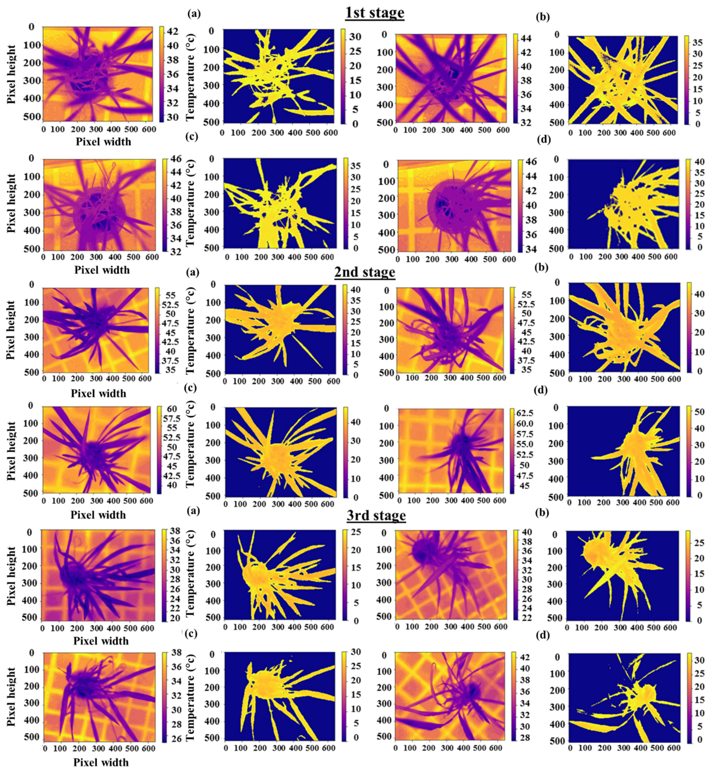
Various objects such as rice plants, soil, and pots were included in the thermal and RGB images collected at the different growth stages of the rice plants. It was necessary to separate the plants and backgrounds for the efficient computation of the canopy water content. Firstly, for the RGB images, a thresholding technique was employed, which is a process of image segmentation to convert the image to grayscale [34] and produce a binary image [34], which has two possible pixel values, namely the intensity value of the image that is more than or equal to the threshold value of 1 (white or foreground) and when it is less than the threshold value or value 0 (black or background) that can be removed. Each pixel in the binary image has a size of 1 bit. After separating the rice pixels from the background objects, a set of candidate features, including color and texture, were extracted for further analysis. Secondly, for the thermal images, python software was employed to generate a code for segmenting the rice plants. The ground temperature was higher than any parts in the image, despite the soil and pot being lower than others. Accordingly, we can separate the temperature of the objects as either higher or lower than that of rice plants. Average plant temperature was calculated for all pixels in each thermal image. Figure 3 describes thermal image segmentation and canopy temperature distribution during the different irrigation treatments in the three growth stages of the rice. At the 1st stage, the canopy temperatures were observed in the ranges of 32–33.5 °C (well-watered), 33.8–35.4 °C (mild stress), 35.75–36.5 °C (moderate stress), and 36.9–37.55 °C (severe stress). The canopy temperature ranges for such treatments at the 2nd stage were 37.5–39.1 °C, 39.22–41.72 °C, 42.39–45.8 °C, and 46.24–48 °C, respectively. Their corresponding values at the 3rd stage were 22.85–24.5 °C, 25–27.7 °C, 28–30.1 °C, and 30.5–33 °C, respectively.

2.5. Feature Extraction from RGB Images

RGB images contain large amounts of data, thereby analyzing the image requires a large volume of memory and leads to more time. Consequently, to decrease the volume of data, an image is depicted using a series of features. The purpose is to capture the image’s certain visual properties. Feature extraction has a crucial role in different image processing systems. The most common ways to extract features from RGB images are RGB color space percentage and GLCM-based texture features.

2.5.1. RGB Color Space Percentage

The RGB imagery involves three bands of red, green, and blue, where each band has a value of each pixel [35]. The rice plants modified the content of chlorophyll to balance photosynthesis and transpiration under conditions of water stress. The RGB channel values were affected, owing to different levels of canopy water content. The percentage values of the RGB color space were determined as typical features using the following formulas:
R = 1 S n u m i = 1 S n u m R i
G = 1 S n u m i = 1 S n u m G i
B = 1 S n u m i = 1 S n u m B i
where R i , G i , and B i are the pixel value for the red, green, and blue band in the digital image, respectively; i and S n u m are the first pixel and the maximum number of pixels, respectively; R, G, and B are mean values of RGB color space.
About 20 color vegetation indices for plant water status estimation were evaluated. Table 2 reveals RGB-based vegetation indices as claimed by numerous previous studies. In our study, these indices were examined to explore their feasibility for CWC modeling and compared as input to the model for adoption of the best indices.

2.5.2. Gray Level Co-Occurrence Matrix-Based Texture Features (GLCMF)

Several studies related to assessing the water status of the plant have used GLCMF: Wenting et al. [21], to predict maize leaf moisture content, and Ushada et al. [46], to estimate the moisture content and leaf water potential of moss. This is based on the fact that changes in the textural appearance of a plant canopy due to the water status reflects tonal variations over the community of plants [47]. The co-occurrence matrix is a statistical method for examining the texture of a grayscale image [48]. The GLCMF analyzes the grayscale relationship between two pixels in the image space that are separated by a certain distance and then randomly extracts the canopy texture feature information premised on probability characteristics. There were six variants of GLCMF in this study such as contrast, dissimilarity, homogeneity, angular second moment (ASM), energy, and correlation. The contrast clearly represents the depth of the image and texture. Dissimilarity measures the distance between pairs of pixels in the region of interest. Homogeneity estimates the closeness of the distribution of elements in the GLCMF. ASM discovers the roughness distribution and texture image. Energy measures textural uniformity. The correlation finds out the degree of correlation in the local grayscale image. The RGB-based GLCMF variables are explicated, as shown in Table 3.

2.6. Feature Extraction from Thermal Images

Thermal indicators (T) are features extracted from thermal images depending on the rice plant temperatures, which consist of two indices in this study: the crop water stress index (CWSI) and normalized relative canopy temperature (NRCT).

2.6.1. Canopy Temperature-Based Crop Water Stress Index (CWSI)

The CWSI deduced from canopy temperature for many crops has been widely nominated as an instrument to elucidate plant water conditions and schedule irrigation [50]. The CWSI concept is linked to the standard in which the leaf surface is cooled during the transpiration process, and as soil moisture in the root zone is also depleted, leaf temperature increases and stomatal transpiration and conductance decrease. An empirical approach was proposed to determine crop water stress as reported by Idso et al. [51]:
CWSI = [ ( T c T a ) ( T nws T a ) ] [ ( T dry T a ) ( T nws T a ) ]
where T a , T c , T nws , and T dry are air temperature ( ° C ), canopy temperature ( ° C ), non-water-stressed canopy temperature ( ° C ), and water-stressed canopy temperature ( ° C ), respectively.

2.6.2. Normalized Relative Canopy Temperature (NRCT)

To calculate the NRCT index, wet-bulb and dry-bulb temperatures were suggested by Jackson et al. [23] as the lower and upper baseline, respectively. As stated in the formula by Elsayed and Darwish [9], the NRCT was computed as follows:
NRCT = T c T min T max T min
where Tmin and Tmax are the lowest and highest temperatures measured in the experiment ( ° C ), respectively.

2.7. Canopy Water Content Computation

After scanning by the visible and thermal imaging system, the plants in each pot were picked. The roots were removed and the rest was studied to provide a reference for data analysis. Thus, the above-ground part of the plants in one pot was defined as one sample in this study. To obtain the fresh weight (FW), the samples were weighed before drying. Then, the dry weight (DW) was obtained after drying the samples for 24 h in an oven at a temperature of 70 °C. The percentage of canopy water content was estimated by the following formula:
CWC   ( % ) = FW DW FW × 100

2.8. Dataset and Data Analysis Software

A total of 120 readings were split into training, validation, and testing, where 80% (96 samples) were used for the training and validation process of the regression model, while the other 20% (24 samples) were used to verify the model’s performance by comparing the expected CWC values with the calculated CWC values. A leave-one-out cross-validation (LOOCV) approach was utilized to train and validate the model. LOOCV excludes one sample for validation and uses the rest of the samples for training in every trial. This method can decrease over-fitting and permits a more accurate assessment of model prediction strength [52]. The feature selection, model establishment, and data analysis were implemented using Python 3.7.3. The ANN module from the Scikit-learn library version 0.20.2 was used for the regression task. The software was run on a PC with Intel Core i7-3630QM, 2.4 GHz CPU, and 8 GB RAM.

2.9. Implementation of a Backpropagation Neural Network (BPNN)

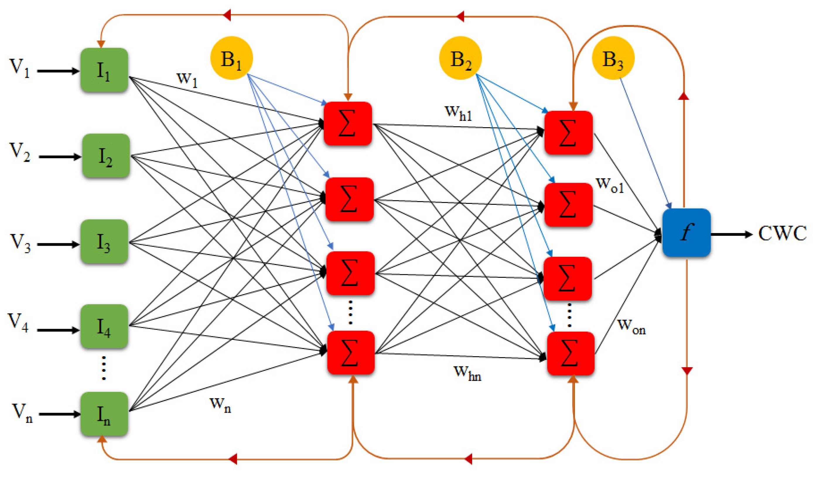
The BPNN employs the multi-layer perceptrons (MLPs) as a supervised learning algorithm that contains a flexible function to train a specific data set [53]. MLP is one of the neural network models that has the same back-propagation structure for supervised training. Typically, back-propagation is used for the training of feed-forward. The neural network is structured from 3 types of layers: (1) the input layer is the primary data for the neural network, (2) the hidden layer is an intermediate layer between the independent inputs layer and dependent output layer, and (3) the output layer produces the results of the specified inputs. Figure 4 displays the architecture of an artificial neural network, which is a class of machine learning algorithms. It uses multiple layers to gradually extract high-level features from the raw input. Five squares as input layers are noted as vector I. The network contains two hidden layers, the number of nodes determined according to regression accuracy. Four squares as hidden layers represent the “activation” nodes and usually are noted as weight; W, Wh, and Wo are with layers 1–2, 2–3, and 3–4, respectively. The final square represents the output layer that shows the predicted value of canopy water content. The bias neuron (B) is a special neuron added to each layer in the neural network, which is usually taken to be 1 [54]. The artificial neural networks are generalized mathematical models that use a series of neurons or nodes interlinked by weighted connections to simulate human cognition as it applies to pattern identification and prediction [55].
Input variants involve RGB-based features (color: 20VI and texture: 6GLCMF) and thermal properties (2T). To facilitate the model training process, a transformation was performed to rescale the features. Normalization is transformed across individual features (f) to adjust for differences in magnitude between different features. Feature normalization (fnorm) is computed by subtracting the minimum image data (fmin) and by dividing the difference between the maximum (fmax) and the minimum feature value as shown by the following formula:
f n o r m = f f m i n f m a x f m i n
The neuron is the primary component of ANN, which involves its elementary mathematical functions. The neuron output (y) can be expressed by the following equation: where Wn indicates the nth weights of the combination that produces the output, θ is the unit step function, W is the weight related with the nth input, and μ is the average.
y   ( θ ) × j = 1 n ( W n μ )
The generalized weight (W) can be realized using the equation below, where i is the index for each covariate of x, o(x) is the predicted outcome probability by covariate vector, and log-odds is a link function for the neural network.
W = l o g ( o ( x ) 1 o ( x ) ) x i
At training, the maximum number of neural network iterations was 1000 iterations. A neural network can stop at exact iterations with the highest network performance. To choose the number of neurons in the hidden layer, the cross-validation technique with the LOOV method was performed on the training dataset. The parameter of limited memory Broyden–Fletcher–Goldfarb–Shanno (lbfgs) was used as a weight optimizer to implement the algorithm efficiently [56]. Otherwise, there are several methodologies to select premium features depending on feature selection algorithms that have become an obvious requirement for prediction and modeling [57]. Glorfeld [58] concluded that an index, such as the following BPNN algorithm in this analysis, can be used to select the most important variables and improves the predictive capacity of the regression model. This index is explicated in the following formula:
M = j = 1 n H [ ( I P j / k = 1 n p   I P j , k ) O j ] i = 1 n p ( j = 1 n H [ ( I P i , j / k = 1 n p   I P i , j , k ) O j ] )
where M is the important measure for the input variable, n p is the number of input variables, n H is the number of hidden layer nodes, I P j is the absolute value of the hidden layer weight corresponding to the pth input variable and the jth hidden layer, and O j is the absolute value of the output layer weight corresponding to the jth hidden layer.

2.10. Hyperparameter Optimization and High-Level Variants Selection

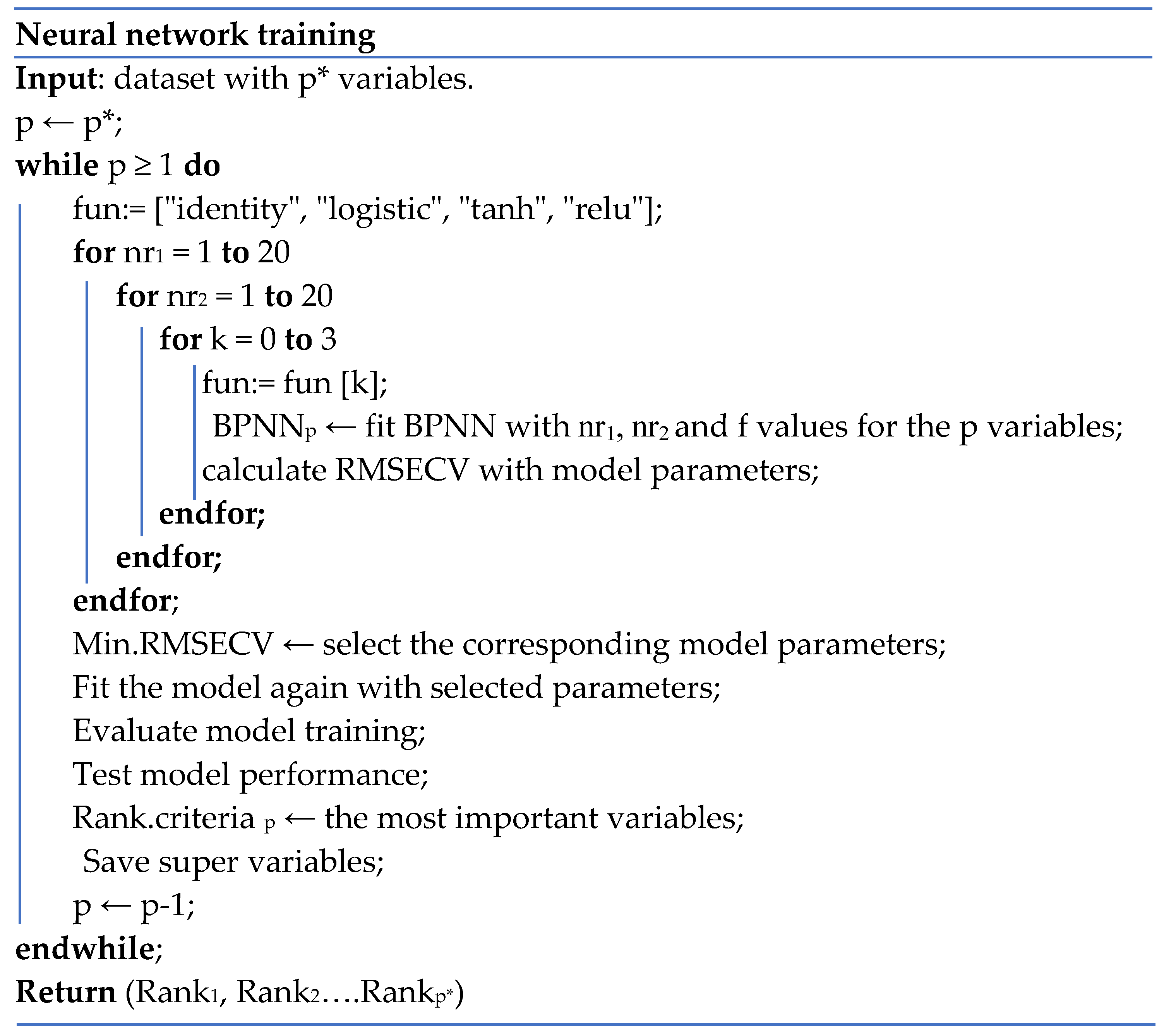
One of the purposes of this research was to compare different features during training the BPNN model. The three types of the dataset (samples×features) for analysis were 120 × 20, 120 × 6, and 120 × 2. These data were employed as input for the neural network. We optimized the model by selecting the prominent hyperparameters. The parameters were the number of neurons in two hidden layers (nr1 and nr2) and activation function (fun). The main steps of neural network training, appropriate hyperparameters estimation, and feature arrangement are described in Figure 5. This figure illustrates the pseudo-code for training a neural net with various variants. The number of features in each loop was with color indices: 20, 19, 18, etc.; texture features: 6, 5, 4, etc.; and thermal indicators: 2, 1. Generally, the variants were fed to the model randomly in the 1st loop, the low-level features were dropped during each loop, and the superb features were organized in ascending order concerning the highest contribution. Then, the ANN outputs were compared to decide high-ranking variants at minimum RMSECV.

2.11. Statistical Analysis Methods

The performance of the artificial neural network was measured through the following selected statistical indicators: mean square error (MSE), root mean square error (RMSE), mean absolute percentage error (MAPE), prediction accuracy (Acc), and coefficient of determination (R2) [59]. All parameters are explicated as follows: CWCact is the actual value that was estimated from laboratory calculations, CWCp is the predicted or simulated value, CWCave is the average value, and NP is the total number of data points.
MSE = 1 Np i = 1 Np ( CWC act CWC p ) 2
RMSE = 1 Np i = 1 Np ( CWC act CWC p ) 2
R 2 = ( CWC act CWC p ) 2 ( CWC act CWC ave ) 2
MAPE = 100 × 1 Np i = 1 Np ( CWC act CWC p ) CWC act
Acc = 1 abs   ( mean   CWC p CWC act CWC act )

3. Results

3.1. Optimization Combinations of Independent Variables Selection

Various combinations of variables were examined to predict CWC, and the top neural network architectures for hidden configurations were presented. The numbers of hidden neurons were different due to the variations in the feature values extracted from the visible and thermal images. The proposed features of color indices, texture characteristics, and thermal indicators were evaluated to adopt the best-combined variants.

3.1.1. Color Vegetation Indices (VI)

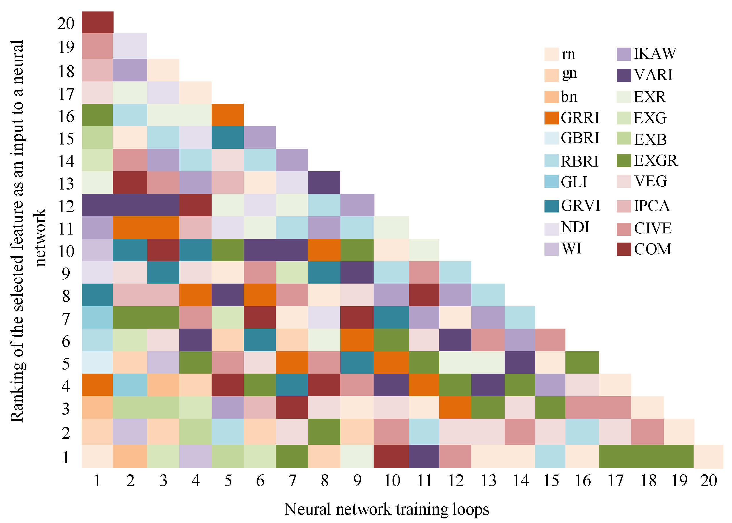
The optimal VI identified in each loop during neural network training are clarified in Figure 6. The neural network performance was estimated with different VI. As explained in Table 4, model performance metrics (MSE, RMSE, and MAPE) were evaluated through training, cross-validation, and a test set. Moreover, the prediction accuracy (Acc) was calculated. The best hyperparameters such as hidden neurons, activation function, and the maximum number of iterations of the neural network were chosen. Several architectures of the BPNN model relying on VI were collected. The best neural network results were attained by fusing data of 14VI at the 7th loop, as displayed in Figure 6. The finest hyperparameters of activation function, hidden neurons, and maximum iterations were logistic, (19,15), and 119 iterations, respectively. The RMSECV decreased to 2.291 vs. 2. 444 compared to 14VI vs. 20VI. The prediction ability of the BPNN-VI-14 model increased equivalent to the model with full VI, with prediction R2 (0.632 vs. 0.556), MAPE (2.832% vs. 3.273%), RMSE (2.788 vs. 3.065), MSE (7.776 vs. 9.394), and Acc (0.972 vs. 0.967).

3.1.2. GLCM-Based Texture Features (GLCMF)

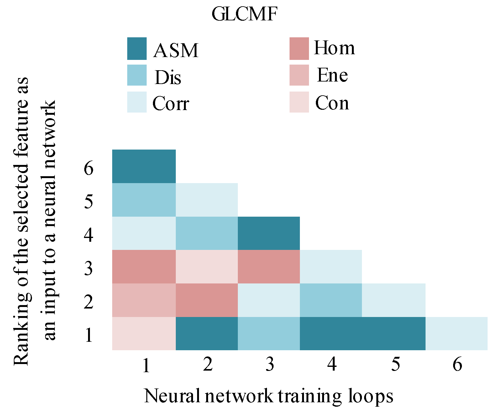
The highest variants of GLCMF selected in each loop are exposed in Figure 7. The different configurations of the GLCMF-based BPNN model and its performance output (MSE, RMSE, and MAPE) with cross-validation, training, and test set are mentioned in Table 5. The optimal neural network was polished by conjoining 5GLCMF at the 2nd loop. The best GLCMF were ASM, homogeneity, contrast, dissimilarity, and correlation, respectively. The ideal parameters of activation function, hidden neurons, and maximum iterations at the fewest value of RMSECV (2.148) were hyperbolic tan, (6,10), and 175 repetitions, respectively. The BPNN-GLCMF-5 model performed better than the BPNN-GLCMF-6 model. The high-level model enhanced the R2 from 0.641 to 0.679, MAPE from 3.151% to 2.938%, RMSE from 2.757 to 2.607, MSE from 7.599 to 6.794, and Acc from 0.968 to 0.971.

3.1.3. Thermal Indicators (T)

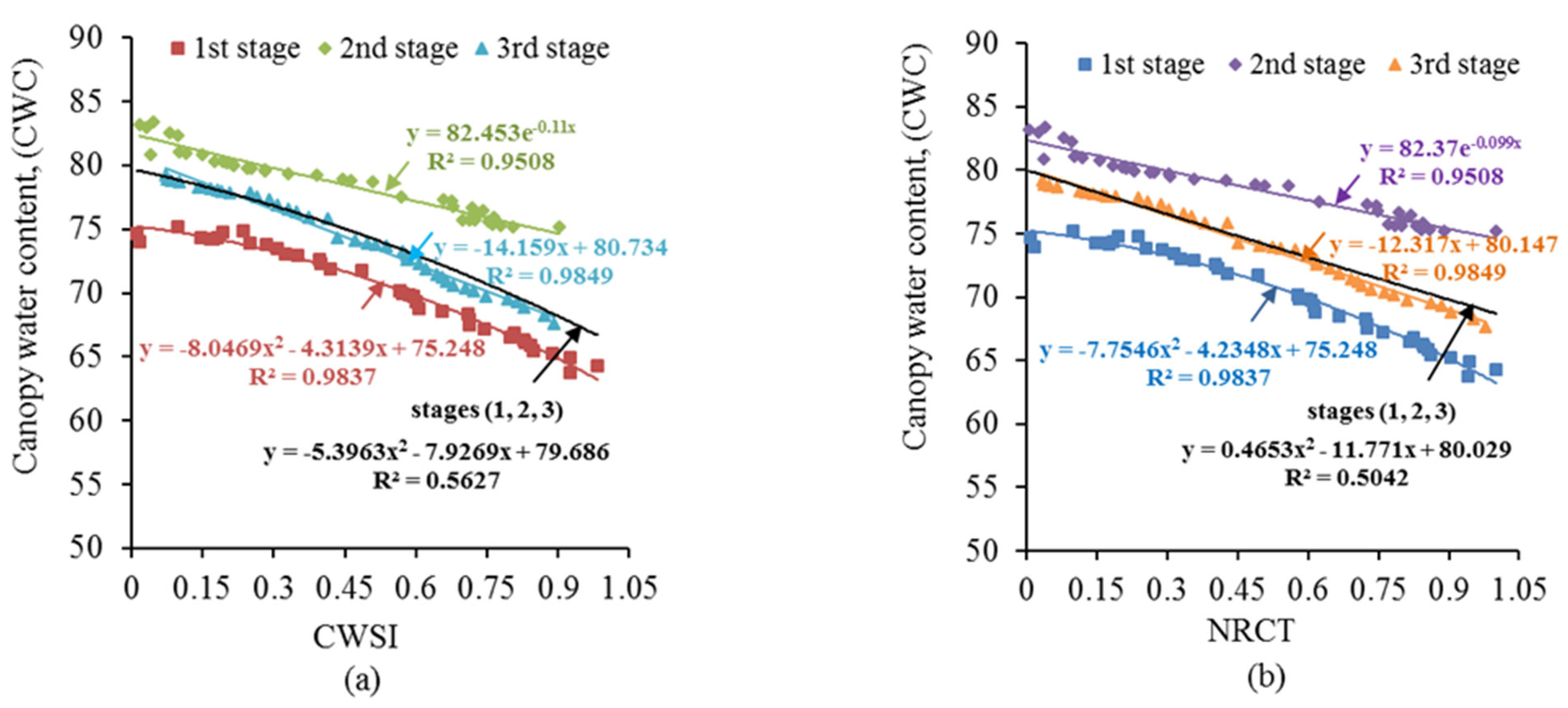
The rice plants, at three growth stages, were grown with four levels of irrigation under outdoor conditions. The temperature of the rice canopy was affected by the water stress. The temperatures of non-water stressed and water-stressed canopy were 31 °C and 38 °C at the 1st stage, 37 °C and 49.1 °C at the 2nd stage, and 22 °C and 34.07 °C at the 3rd stage, respectively. We exploited the previous temperatures for computing the two thermal indicators: CWSI and NRCT. The relationship of both CWSI and NRCT with the CWC of rice at each growth stage is designated in Figure 8. It was observed to be inversely related, and the R2 at each stage independently was higher than the R2 at three stages. By applying ANN with thermal indicators, the prediction formula to compute the CWC at any stage of rice growth was explored with high accuracy. The neural network outputs with thermal indicators at the 1st and 2nd loop are illuminated in Table 6. It depicts the optimal parameters of the T-based BPNN model and its outputs (R2, MAPE, RMSE, MSE, and Acc) through cross-validation, training, and test set. The results approved that the BPNN-CWSI-NRCT was a high-quality model for CWC computation (R2 = 0.803, MAPE = 1.989%, RMSE = 2.043, MSE = 4.172, and Acc = 0.980) as opposed to BPNN-CWSI (R2 = 0.505, MAPE = 3.782%, RMSE = 3.239, MSE = 10.473, and Acc = 0.962). The RMSECV decreased from 2.549 to 1.116 against 1 and 2T, respectively. The model of BPNN-T-2 was excellent for estimating the CWC by (19,18) neurons in two hidden layers, logistic as activation function, and 217 duplications.

3.1.4. Best-Combined Features Extracted from Visible and Thermal Imagery

The findings inferred that in comparison with the BPNN-GLCMF-5 and BPNN-VI-14 models, the BPNN-T-2 model had dependable foretelling. Further, the thermal indicators (T) were joined with VI and GLCMF to improve the forecasting performance and discover the unmatched model. The three approaches were espoused as a new expectation procedure of the rice water content, incorporating VI-T, GLCMF-T, and VI-GLCMF-T features with the BPNN model. Their outputs (MSE, RMSE, and MAPE) and notable parameters are disclosed in Table 7. The order of the models was defined by the smallest RMSECV: the performance of BPNN-VI-GLCMF-T-21>BPNN-GLCM-T-7>BPNN-VI-T-16. Their corresponding values at cross-validation R2 were 0.984 (RMSECV = 0.361), 0.982 (RMSECV = 0.447), and 0.956 (RMSECV = 0.661), respectively. Their prediction outputs with the R2, MAPE, RMSE, MSE, and Acc were 0.983, 0.564%, 0.599, 0.359, and 0.994; 0.972, 0.668%, 0.764, 0.583, and 0.993; and 0.978, 0.682%, 0.674, 0.455, and 0.993, respectively. The distinguishing parameters of the most robust model were with hidden layer neurons (8,9), activation function (logistic), and maximum iterations (422). The BPNN-VI-GLCM-T-21 model had quick predictive outcomes within 31.911 s for a single sample compared to the oven-drying method [17,60]; a test time of 24 h is required to dry the sample. The findings are in agreement with Meeradevi et al. [61] who used ANN as a fast tool with a prediction time of 9.74 s. The results elucidated that the improvement in prediction accuracy of CWC can be fulfilled if adequate neural network parameters and higher variables are assigned.

3.2. Neural Network Learning Curves with Super Features

The learning curve of the regression model was promoted in this study through the following considerations: (1) number and characteristics of nominated features, (2) picking the supreme parameters, and (3) neural network definite iterations to avoid model over-fitting. The first two points are discussed in the previous sections. The last factor refers to the neural network stopping at specific iterations that can progress the network performance, as indicated in Figure 9. These curves exhibit an evaluation of the model’s behavior with the higher variants at training, cross-validation, and testing. As the number of iterations increases, the accuracies of training, cross-validation, and testing increase gradually to reach a point where the learning curves show a good model. As publicized in Figure 9a–d, the optimal repetitions of the BPNN training process through the highest variables (14VI, 5GLCMF, 2T, and VI-GLCMF-T-21) were 119, 175, 217, and 422 steps, respectively. The learning curves of the innovative models reached a cross-validation accuracy of 0.625, 0.656, 0.851, and 0.984, respectively. The learning outcomes verified that the accuracy measure steadily increases over iterations of training. When the permissible iterations of the neural network are exceeded, the model generally takes the form of making an overly complex model. Moreover, training accuracy was usually higher than cross-validation accuracy. The three-stage model of BPNN-VI-GLCMF-T was accomplished with 21 variables and 422 steps. Its prediction accuracy was 99.4% (R2 = 0.983 with an RMSE of 0.599), and the learning curve performance was impressive (Figure 9d). The expected performance was improved as said by Thawornwong and Enke [62]; to avoid over-fitting, the network was trained by the back-propagation algorithm with early stopping.

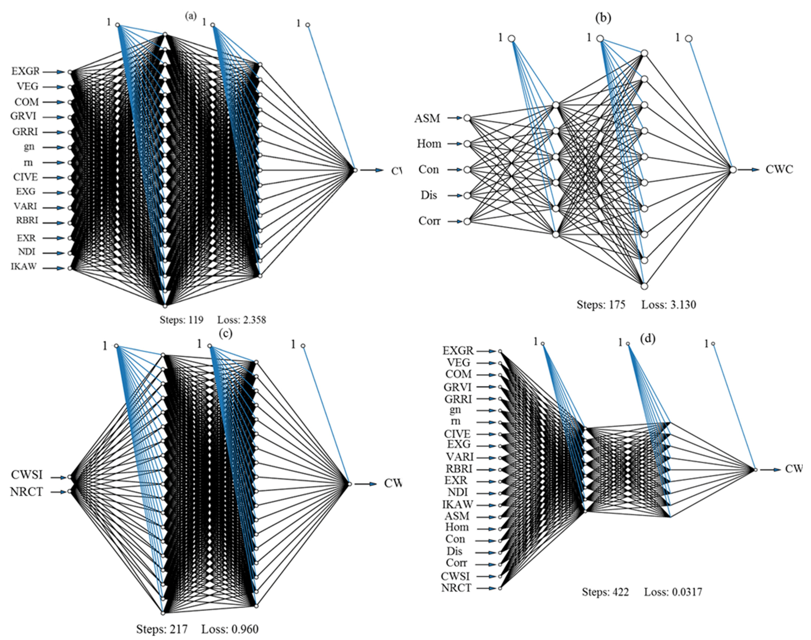
3.3. Neural Network Topology with Higher Variants

The neural network architectures after gathering senior features are introduced in Figure 10. This figure showed the best neural network structure with the variants chosen. Each network topology offers basic information such as the synaptic weights trained, a range of hidden neuron layers, steps for converging, and the overall errors. The network topology is constructed with a specific combination of input variables with a number of hidden neuron layers. For instance, the model of BPNN-VI-14 had hidden neuron layers (19,15), BPNN-GLCMF-5 needed (6,10), BPNN-T-2 required (19,18), and BPNN-VI-GLCMF-T-21 desired (8,9). The layout presented in Figure 10a depicts the BPNN-VI-14 model; the training process needed 119 steps to achieve a lower error function. The process has an overall error of roughly 2.358. The learning process of the BPNN-GLCMF-5 model (Figure 10b) demands 175 steps, containing an overall error of about 3.130. At the BPNN-T-2 model (Figure 10c), the training process obligated 217 steps with a total error of about 0.960. At the BPNN-VI-GLCMF-T-21 model (Figure 10d), the learning process requested 422 steps, and the overall error was 0.0317.

3.4. Canopy Water Content Prediction and Validation

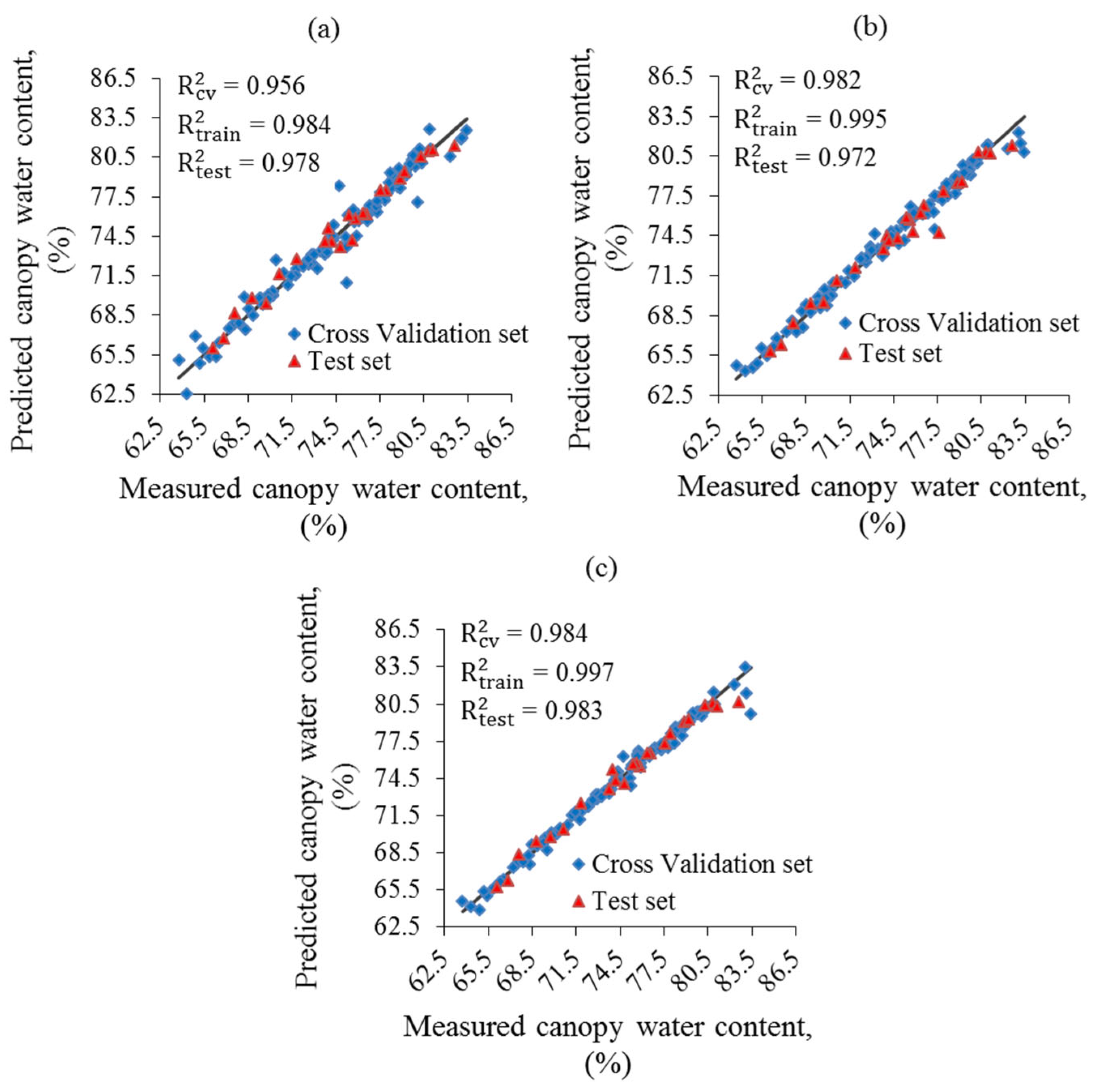
From the results, the thermal features had a high ranking for measuring the CWC of rice in contrast to VI and GLCMF. The super thermal variables were linked to acceptable-level features as follows: VI-GLCMF-T, VI-T, and GLCM-T. The VI-GLCMF-T features were the premium integration to filter the uppermost variables. The neural network was trained with the previous features (independent variables) for predicting the CWC (dependent variable). The expected CWC values were then compared with the reserved values not implemented for the neural network. Figure 11 illustrates the scatter plots of observed and predicted CWC in rice exploiting the proposed features. This study evaluated multivariate methods and compared the results clearly, so the use of multivariate methods greatly enhances predictability. Independent validation can also be considered the most robust method for evaluating the accuracy of the regression model since validation data are not involved in the model development process. The BPNN-VI-GLCMF-T-21 was the first best predictive model as evidenced by the performance and showed a stronger relationship between the superlative features and CWC. These features involved in this model are of great significance for predicting water content. Its outputs with R2 were 0.984 (cross-validation) and 0.983 (test set). The BPNN-GLCMF-T-7 model ranked second in performance. The R2 value was 0.982 and 0.972 in the cross-validation and test set, respectively. The BPNN-VI-T-16 was the third highest accurate model (R2 = 0.956 and 0.978 for cross-validation and test set, respectively). Models constructed with individual features of either VI or GLCMF had lower performance expectations, while these features combined with 2T achieved robust forecasting. Otherwise, the residual value plays a vital role to validate the obtained regression model. The difference between the actual CWC and the predicted CWC value is the residual. We calculated the residual value with the first three higher models. At BPNN-VI-GLCM-T-21, −1.223% and 1.916% were the lowest and highest residuals for the CWC prediction, respectively. At BPNN-VI-T-16, the lowest and highest residuals were −1.128% and 1.380%, while the lowest residuals of −0.583% and highest of 2.859% were calculated with BPNN-GLCMF-T-7.

4. Discussion

Color and texture are two important aspects in digital imagery. Plant temperature is also a remarkable tool in thermal imaging, which can be used as an indicator to identify a plant’s water condition. The plant color feature can be used for plant stress assessment [63]. Texture analysis is significant in many areas such as remote sensing and its common applications include image classification and pattern recognition [64]. These features of VI and GLCMF were applied with a neural network for CWC quantification in rice. The results confirmed that the neural network behavior with GLCMF was superior to VI for predicting the water status of plants. This is similar to applying classification in the following studies: Jana et al. [65], to classify eight varieties of fruits, and Dubey and Jalal [66], to recognize diseases in fruits. Texture features performed better than color features for classification via support vector machine algorithm with accuracy, 32.29% and 69.79% and 83.5% and 88.56%, respectively. Moreover, the thermal analysis results agreed with the findings of Jones [67], who identified that water content or transpiration has an inverse relationship with leaf temperature. The CWC values were highly influenced owing to the loss of water through transpiration; CWSI and NRCT reflected normalized temperature values for the crop. These results are in agreement with Blum et al. [68], who indicated that the CWC decreases with increasing canopy temperature as a result of increased water stress.
The current work has allowed a more accurate determination of the water conditions in rice, using the best-combined features extracted from RGB and thermal images. The proposed approaches use all of the sensitive features to changes in the CWC that greatly increase the model performance. Our outcomes achieved greater accuracy than those of Alchanatis et al. [69], who demonstrated that fusion of thermal and visible imaging can provide precise data on the crop water status of grapevines, and the CWSI was highly correlated with measured stomatal conductance with an R2 value of 0.97. The developed model outperformed Leinonen and Jones [70], who stated that the combination of thermal and visible imagery was a more accurate tool for estimating canopy temperature and could be used to identify water deficit stress in a plant. They investigated the relationship between the measured stomatal conductance and the calculated CWSI with an R2 of 0.867. Likewise, the first-order model of the BPNN-VI-GLCM-T-21 was very precise in contrast to that of Sun et al. [71], who referred to a reasonable model for computing CWC in wheat based on the ratio vegetation index (RVI: 1605 and 1712 nm) and the normalized difference vegetation index (NDVI: 1712 and 1605 nm), having the highest R2 and lowest RMSE in model calibration and validation (R2c = 0.74 and 0.73; RMSEC = 0.026 and 0.027; R2v = 0.72 and 0.71; RMSEV = 0.028 and 0.029). Furthermore, the proposed model is better than Ge et al. [72], who concluded that leaf water content in maize at a pot-scale is successfully predicted with the hyperspectral images using the PLSR model for two genotypes in model cross-validation (R2 = 0.81 and 0.92; RMSE = 3.7 and 2.3; MAPE = 3.6 and 2.2). The created model achieved high performance compared to Pandey et al. [73], who reported that PLSR analysis can be performed to predict the leaf water content of pot-grown maize and soybean plants with the highest accuracy (R2 = 0.93, RMSE = 1.62, and MAPE = 1.6%) for validation. In addition, this research is in agreement with the following study in that the combination of color–GLCM–thermal features are high-quality variants in regression or classification applications. Bhole et al. [74] used different features such as the color (CM: color moments and CCV: color coherence vector), texture (GLCMF), and thermal (T) with a random forest for classification of eleven categories of fruits. The results showed that the model accuracies for integrating GLCM-T, CM-T, CCV-T, and CM-CCV-GLCM-T features were 84.26%, 91.17%, 92.95%, and 93.4%, respectively.
Finally, remote and proximal sensing images acquired with high-resolution cameras, mounted at ground level or on unmanned aerial vehicles (UAV), have spatial resolutions of a few centimeters. These images can provide sufficient accurate information for both assessing plant water status in the field and implementing appropriate irrigation management strategies [75]. Thus, this work can assist in improving inexpensive, effective high-throughput phenotyping platforms for large numbers of breeding plants at different levels of irrigation. A practical sharing of research may improve site-specific rice irrigation management through designing an intelligent irrigation system based on the best-proposed model. The methodology of this study that relied on ground-based cameras can be scaled up to UAV-based applications to increase productivity [76] and monitor the water condition of crops in large-scale areas.

5. Conclusions

Estimation of canopy water content (CWC) is highly important in precision plant reproduction and agricultural development. Low-cost outdoor cameras, such as visible and thermal imaging systems, would be an applicable implement for predicting water content in the plant. Therefore, the present study explored the ability to incorporate top-level features retrieved from visible and thermal imaging with a back-propagation neural network (BPNN) to adopt a three-stage model of CWC for rice. Hand-crafted features, including 20 vegetation indices (VI), 6 GLCM texture features (GLCMF), and 2 thermal indicators (T), were identified for analysis. The experimental results showed that the proposed model of BPNN-VI-GLCMF-T provided effective recognition of CWC in the rice crop. Expectation accuracy increased to 99.4% by conjoining 21 superlative features. At hidden neuron layers (8,9), the R2 raised to 0.983 with an RMSE of 0.599. The models with separate features performed lower than the best built-in features. Their corresponding values with prediction R2 were 0.632 (RMSE = 2.788), 0.679 (RMSE = 2.607), and 0.803 (RMSE = 2.043) using 14VI, 5GLCM, and 2T, respectively. Ultimately, the superlative model has a high level of confidence and reliable outcomes. In the future, this tool may open an avenue for rapid, high-throughput assessments of the water condition of plants, as well as being equally important for procedures related to agricultural water management.

Author Contributions

O.E. implemented the experiment, data curation, software, and prepared the original draft for writing the manuscript. L.Z. collected the data and revised the manuscript. L.F. reviewed, edited the manuscript, and provided funding for the project. Z.Q. planned the overall study, supervised the research, reviewed, edited the manuscript, and supplied the funding. All authors have read and agreed to the published version of the manuscript.

Funding

This work was supported by China National Key Research and Development Program (2016YFD0700304), XPCC Science and Technology Projects of Key Areas (2020AB005), and National Natural Science Foundation of China (31871526).

Data Availability Statement

The data presented in this study are available within the article.

Conflicts of Interest

The authors declare no conflict of interest.

References

  1. Gilbert, N. Water under pressure. Nat. Cell Biol. 2012, 483, 256–257. [Google Scholar] [CrossRef] [PubMed] [Green Version]
  2. El-Hendawy, S.; Al-Suhaibani, N.; Salem, A.; Ur Rehman, S.; Schmidhalter, U. Spectral reflectance indices as a rapid nondestructive phenotyping tool forestimating different morphophysiological traits of contrasting spring wheatgermplasms under arid conditions. Turk. J. Agric. For. 2015, 39, 572–587. [Google Scholar] [CrossRef]
  3. Guerra, L.C.; Bhuiyan, S.I.; Tuong, T.P.; Barker, R. Producing More Rice with Less Water from Irrigated Systems; SWIM Paper 5; IWMI/IRRI: Colombo, Sri Lanka, 1998. [Google Scholar]
  4. Liu, Y.; Liang, Y.; Deng, S.; Li, F. Effects of irrigation method and radio of organic to inorganic nitrogen on yield ann water use of rice. Plant Nutr. Fertil. Sci. 2012, 18, 551–561. [Google Scholar]
  5. Clevers, J.G.P.W.; Kooistra, L.; Schaepman, M.E. Estimating canopy water content using hyperspectral remote sensing data. Int. J. Appl. Earth. Obs. 2010, 12, 119–125. [Google Scholar] [CrossRef]
  6. Penuelas, J.; Filella, I.; Serrano, L.; Save, R. Cell wall elasticity and water index (r970nm/r900nm) in wheat under different nitrogen availabilities. Int. J. Remote Sens. 1996, 17, 373–382. [Google Scholar] [CrossRef]
  7. Hank, T.B.; Berger, K.; Bach, H.; Clevers, J.G.P.W.; Gitelson, A.; Zarco-Tejada, P.; Mauser, W. Spaceborne imaging spectroscopy for sustainable agriculture: Contributions and challenges. Surv. Geophys. 2019, 40, 515–551. [Google Scholar] [CrossRef] [Green Version]
  8. Peñuelas, J.; Pinol, J.; Ogaya, R.; Filella, I. Estimation of plant water concentration by the reflectance water index wi (r900/r970). Int. J. Remote Sens. 1997, 18, 2869–2875. [Google Scholar] [CrossRef]
  9. Elsayed, S.; Darwish, W. Hyperspectral remote sensing to assess the water status, biomass, and yield of maize cultivars under salinity and water stress. Bragantia. 2017, 76, 62–72. [Google Scholar] [CrossRef] [Green Version]
  10. Scholander, P.F.; Bradstreet, E.D.; Hemmingsen, E.A.; Hammel, H.T. Sap Pressure in Vascular Plants: Negative hydrostatic pressure can be measured in plants. Science. 1965, 148, 339–346. [Google Scholar] [CrossRef]
  11. Agam, N.; Cohen, Y.; Berni, J.; Alchanatis, V.; Kool, D.; Dag, A.; Yermiyahu, U.; Ben-Gal, A. An insight to the performance of crop water stress index for olive trees. Agric. Water Manag. 2013, 118, 79–86. [Google Scholar] [CrossRef]
  12. Singh, A.K.; Madramootoo, C.A.; Smith, D.L. Water Balance and Corn Yield under Different Water Table Management Scenarios in Southern Quebec. In Proceedings of the 9th International Drainage Symposium Held Jointly with CIGR and CSBE/SCGAB, Quebec City, QC, Canada, 13–16 June 2010. [Google Scholar]
  13. Rud, R.; Cohen, Y.; Alchanatis, V.; Levi, A.; Brikman, R.; Shenderey, C.; Heuer, B.; Markovitch, T.; Dar, Z.; Rosen, C.; et al. Crop water stress index derived from multi-year ground and aerial thermal images as an indicator of potato water status. Precis. Agric. 2014, 15, 273–289. [Google Scholar] [CrossRef]
  14. Dhillon, R.S.; Upadhaya, S.K.; Rojo, F.; Roach, J.; Coates, R.W.; Delwiche, M.J. Development of a continuous leaf monitoring system to predict plant water status. T. ASABE. 2017, 60, 1445–1455. [Google Scholar] [CrossRef]
  15. Prey, L.; von Bloh, M.; Schmidhalter, U. Evaluating RGB imaging and multispectral active and hyperspectral passive sensing for assessing early plant vigor in winter wheat. Sensors 2018, 18, 2931. [Google Scholar] [CrossRef] [Green Version]
  16. Li, L.; Zhang, Q.; Huang, D. A review of imaging techniques for plant phenotyping. Sensors 2014, 14, 20078–20111. [Google Scholar] [CrossRef]
  17. Elsherbiny, O.; Fan, Y.; Zhou, L.; Qiu, Z. Fusion of feature selection methods and regression algorithms for predicting the canopy water content of rice based on hyperspectral data. Agriculture 2021, 11, 51. [Google Scholar] [CrossRef]
  18. Woebbecke, D.M.; Meyer, G.E.; Von Bargen, K.; Mortensen, D. Color indices for weed identification under various soil, residue, and lighting conditions. Trans. ASAE. 1995, 38, 259–269. [Google Scholar] [CrossRef]
  19. Wang, F.Y.; Wang, K.R.; Wang, C.T.; Li, S.K.; Zhu, Y.; Chen, B. Diagnosis of cotton water status based on image recognition. J. Shihezi Univ. Nat. Sci. 2007, 25, 404–408. [Google Scholar]
  20. Zakaluk, R.; Sri, R.R. Predicting the leaf water potential of potato plants using RGB reflectance. Can. Biosyst. Eng. 2008, 50. [Google Scholar]
  21. Wenting, H.; Yu, S.; Tengfei, X.; Xiangwei, C.; Ooi, S.K. Detecting maize leaf water status by using digital RGB images. Int. J. Agric. Biol. Eng. 2014, 7, 45–53. [Google Scholar]
  22. Shao, Y.; Zhou, H.; Jiang, L.; Bao, Y.; He, Y. Using reflectance and gray-level texture for water content prediction in grape vines. T. ASABE. 2017, 60, 207–213. [Google Scholar]
  23. Jackson, R.D.; Idso, S.; Reginato, R.; Pinter, P. Canopy temperature as a crop water stress indicator. Water Resour. Res. 1981, 17, 1133–1138. [Google Scholar] [CrossRef]
  24. Moller, M.; Alchanatis, V.; Cohen, Y.; Meron, M.; Tsipris, J.; Naor, A.; Ostrovsky, V.; Sprintsin, , M.; Cohen , S. Use of thermal and visible imagery for estimating crop water status of irrigated grapevine. J. Exp. Bot. 2006, 58, 827–838. [Google Scholar] [CrossRef] [Green Version]
  25. Ballester, C.; Jiménez-Bello, M.A.; Castel, J.R.; Intrigliolo, D.S. Usefulness of thermography for plant water stress detection in citrus and persimmon trees. Agric. Forest Meteorol. 2013, 168, 120–129. [Google Scholar] [CrossRef]
  26. Melis, G.; Dyer, C.; Blunsom, P. On the state of the art of evaluation in neural language models. arXiv 2017, arXiv:1707.05589. [Google Scholar]
  27. Bergstra, J.; Yamins, D.; Cox, D. Making a Science of Model Search: Hyperparameter Optimization in Hundreds of Dimensions for Vision Architectures. In Proceedings of the 30th International Conference on Machine Learning (ICML 2013), Atlanta, GA, USA, 16–21 June 2013; pp. 115–123. [Google Scholar]
  28. Wu, J.; Chen, X.-Y.; Zhang, H.; Xiong, L.-D.; Lei, H.; Deng, S.-H. Hyperparameter optimization for machine learning models based on Bayesian optimization. JEST 2019, 17, 26–40. [Google Scholar]
  29. Dawson, T.P.; Curran, P.J.; Plummer, S.E. LIBERTY—Modelling the effects of leaf biochemical concentration on reflectance spectra. Remote Sens. Environ. 1998, 65, 50–60. [Google Scholar] [CrossRef]
  30. Marti, P.; Gasque, M.; Gonzalez-Altozano, P. An artificial neural network approach to the estimation of stem water potential from frequency domain reflectometry soil moisture measurements and meteorological data. Comput. Electron. Agric. 2013, 91, 75–86. [Google Scholar] [CrossRef]
  31. Abtew, W.; Melesse, A. Evaporation and evapotranspiration: Measurements and estimations. Springer Sci. 2013, 53, 62. [Google Scholar]
  32. Costa, J.M.; Grant, O.M.; Chaves, M.M. Thermography to explore plant-environment interactions. J. Exp. Bot. 2013, 64, 3937–3949. [Google Scholar] [CrossRef]
  33. Li, H.; Malik, M.H.; Gao, Y.; Qiu, R.; Miao, Y.; Zhang, M. Proceedings of the Maize Plant Water Stress Detection Based on RGB Image and Thermal Infrared Image, Detroit, MI, USA, 29 July–1 August 2018.
  34. Yossya, E.H.; Pranata, J.; Wijaya, T.; Hermawan, H.; Budiharto, W. Mango fruit sortation system using neural network and computer vision. Procedia Comput. Sci. 2017, 116, 569–603. [Google Scholar] [CrossRef]
  35. Kumaseh, M.R.; Latumakulita, L.; Nainggolan, N. Segmentasi citra digital ikan menggunakan metode thresholding. J. Ilmiah Sains. 2013, 13, 74–79. [Google Scholar] [CrossRef] [Green Version]
  36. Kawashima, S.; Nakatani, M. An algorithm for estimating chlorophyll content in leaves using a video camera. Ann. Bot. 1998, 81, 49–54. [Google Scholar] [CrossRef] [Green Version]
  37. Verrelst, J.; Schaepman, M.E.; Koetz, B.; Kneubuhler, M. Angular sensitivity analysis of vegetation indices derived from CHRIS/PROBA data. Remote Sens. Environ. 2008, 112, 2341–2353. [Google Scholar] [CrossRef]
  38. Sellaro, R.; Crepy, M.; Trupkin, S.A.; Karayekov, E.; Buchovsky, A.S.; Rossi, C.; Casal, J.J. Cryptochrome as a sensor of the blue/green ratio of natural radiation in Arabidopsis. Plant Physiol. 2010, 154, 401–409. [Google Scholar] [CrossRef] [PubMed] [Green Version]
  39. Woebbecke, D.; Meyer, G.; Von Bargen, K.; Mortensen, D. Plant Species Identification, Size, and Enumeration using Machine Vision Techniques on Near-Binary Images. In Proceedings of the Optics in Agriculture and Forestry, Boston, MA, USA, 16–17 November 1992; Volume 1836, pp. 208–219. [Google Scholar]
  40. Tucker, C.J. Red and photographic infrared linear combinations for monitoring vegetation. Remote Sens. Environ. 1979, 8, 127–150. [Google Scholar] [CrossRef] [Green Version]
  41. Louhaichi, M.; Borman, M.M.; Johnson, D.E. Spatially located platform and aerial photography for documentation of grazing impacts on wheat. Geocarto Int. 2001, 16, 65–70. [Google Scholar] [CrossRef]
  42. Gitelson, A.A.; Kaufman, Y.J.; Stark, R.; Rundquist, D. Novel algorithms for remote estimation of vegetation fraction. Remote Sens. Environ. 2002, 80, 76–87. [Google Scholar] [CrossRef] [Green Version]
  43. Mao, W.; Wang, Y.; Wang, Y. Real-Time Detection of between-Row Weeds using Machine Vision. In Proceedings of the 2003 ASAE Annual Meeting, Las Vegas, NV, USA, 27–30 July 2003; p. 1. [Google Scholar]
  44. Saberioon, M.M.; Amin, M.S.M.; Anuar, A.R.; Gholizadeh, A.; Wayayok, A.; Khairunniza- Bejo, S. Assessment of rice leaf chlorophyll content using visible bands at different growth stages at both the leaf and canopy scale. Int. J. Appl. Earth Obs. Geoinf. 2014, 32, 35–45. [Google Scholar] [CrossRef]
  45. Guijarro, M.; Pajares, G.; Riomoros, I.; Herrera, P.J.; Burgos-Artizzu, X.P.; Ribeiro, A. Automatic segmentation of relevant textures in agricultural images. Comput. Electron. Agric. 2011, 75, 75–83. [Google Scholar] [CrossRef] [Green Version]
  46. Ushada, M.; Murase, H.; Fukuda, H. Non-destructive sensing and its inverse model for canopy parameters using texture analysis and artificial neural network. Comput. Electron. Agric. 2007, 57, 149–165. [Google Scholar] [CrossRef]
  47. Murase, H.; Tani, A.; Nishiura, Y.; Kiyota, M. Growth Monitoring of Green Vegetables Cultured in a Centrifuge Phytotron. In Plant Production in Closed Ecosystems; Goto, E., Kurata, K., Hayashi, M., Sase, S., Eds.; Kluwer Academic Publishers: Amsterdam, The Netherlands, 1997; pp. 305–319. [Google Scholar]
  48. Athanasiou, L.S.; Fotiadis, D.I.; Michalis, L.K. Plaque Characterization Methods using Intravascular Ultrasound Imaging. In Atherosclerotic Plaque Characterization Methods Based on Coronary Imaging, 1st ed.; Elsevier: Amsterdam, The Netherlands, 2017; pp. 71–94. [Google Scholar]
  49. Hall-Beyer, M. GLCM Texture: A Tutorial v. 1.0 through 2.7. Available online: http://hdl.handle.net/1880/51900 (accessed on 4 April 2017).
  50. Bellvert, J.; Marsal, J.; Girona, J.; Gonzalez-Dugo, V.; Fereres, E.; Ustin, S.L.; Zarco-Tejada, P.J. Airborne thermal imagery to detect the seasonal evolution of crop water status in peach, nectarine and Saturn peach orchards. Remote Sens. 2016, 8, 39. [Google Scholar] [CrossRef] [Green Version]
  51. Idso, S.B.; Jackson, R.D.; Pinter, P.J.; Reginato, R.J.; Hatfield, J.L. Normalizing the stress degree-day parameter for environmental variability. Agric. Meteorol. 1981, 24, 45–55. [Google Scholar] [CrossRef]
  52. Zhu, J.; Huang, Z.H.; Sun, H.; Wang, G.X. Mapping forest ecosystem biomass density for Xiangjiang river basin by combining plot and remote sensing data and comparing spatial extrapolation methods. Remote Sens. 2017, 9, 241. [Google Scholar] [CrossRef] [Green Version]
  53. Kisi, O.; Demir, V. Evapotranspiration estimation using six different multi-layer perceptron algorithms. Irrig. Drain. Syst. Eng. 2016, 5, 991–1000. [Google Scholar] [CrossRef]
  54. Barndorff-Nielsen, O.E.; Jensen, J.L.; Kendall, W.S. Networks and Chaos: Statistical and Probabilistic Aspects; Chapman and Hall: London, UK, 1993; Volume 50, p. 48. [Google Scholar]
  55. Li, J.; Yoder, R.; Odhiambo, L.O.; Zhang, J. Simulation of nitrate distribution under drip irrigation using artificial neural networks. Irrigation Sci. 2004, 23, 29–37. [Google Scholar] [CrossRef]
  56. Byrd, R.H.; Lu, P.; Nocedal, J.; Zhu, C. A limited memory algorithm for bound constrained optimization. Siam J. Sci. Comput. 1995, 16, 1190–1208. [Google Scholar] [CrossRef]
  57. Schuize, F.H.; Wolf, H.; Jansen, H.W.; Vander, V.P. Applications of artificial neural networks in integrated water management: Fiction or future? Water Sci. Technol. 2005, 52, 21–31. [Google Scholar] [CrossRef]
  58. Glorfeld, L.W. A methodology for simplification and interpretation of backpropagation-based neural network models. Expert Syst. Appl. 1996, 10, 37–54. [Google Scholar] [CrossRef]
  59. Saggi, M.K.; Jain, S. Reference evapotranspiration estimation and modeling of the Punjab Northern India using deep learning. Comput. Electron. Agric. 2019, 156, 387–398. [Google Scholar] [CrossRef]
  60. Panigrahi, N.; Das, B.S. Evaluation of regression algorithms for estimating leaf area index and canopy water content from water stressed rice canopy reflectance. Inf. Process. Agric. 2020. [Google Scholar] [CrossRef]
  61. Meeradevi; Sindhu, N.; Mundada, M.R. Machine learning in agriculture application: Algorithms and techniques. IJITEE 2020, 9, 2278–3075. [Google Scholar]
  62. Thawornwong, S.; Enke, D. The adaptive selection of financial and economic variables for use with artificial neural networks. Neurocomputing 2004, 56, 205–232. [Google Scholar] [CrossRef]
  63. Bai, G.; Jenkins, S.; Yuan, W.; Graef, G.L.; Ge, Y. Field-based scoring of soybean iron deficiency chlorosis using RGB imaging and statistical learning. Front. Plant Sci. 2018, 9, 1002. [Google Scholar] [CrossRef] [Green Version]
  64. Bharati; Manish, H.; Liu, J.J.; MacGregor, J.F. Image texture analysis: Methods and comparisons. Chemometr. Intell. Lab. 2004, 72, 57–71. [Google Scholar] [CrossRef]
  65. Jana, S.; Basak, S.; Parekh, R. Automatic fruit recognition from natural images using color and texture features. In Proceedings of the 2017 Devices for Integrated Circuit (DevIC), Kalyani, India, 23–24 March 2017; pp. 620–624. [Google Scholar]
  66. Dubey, S.R.; Jalal, A.S. Fusing color and texture cues to identify the fruit diseases using images. Int. J. Comput. Vis. Image Process. 2014, 4, 52–67. [Google Scholar] [CrossRef]
  67. Jones, H.G. Plants and Microclimate, 2nd ed.; Cambridge University Press: Cambridge, UK, 1992. [Google Scholar]
  68. Blum, A.; Mayer, J.; Gozlan, G. Infrared thermal sensing of plant canopies as a screening technique for dehydration avoidance in wheat. Field Crop. Res. 1982, 5, 137–146. [Google Scholar] [CrossRef]
  69. Alchanatis, V.; Cohen, Y.; Cohen, S.; Moller, M.; Meron, M.; Tsipris, J.; Orlov, V.; Naor, A.; Charit, Z. Fusion of IR and multispectral images in the visible range for empirical and model based mapping of crop water status. In Proceedings of the 2006 ASAE Annual Meeting, Portland, OR, USA, 9–12 July 2006; p. 1. [Google Scholar]
  70. Leinonen, I.; Jones, H.G. Combining thermal and visible imagery for estimating canopy temperature and identifying plant stress. J. Exp. Bot. 2004, 55, 1423–1431. [Google Scholar] [CrossRef] [Green Version]
  71. Sun, H.; Feng, M.; Xiao, L.; Yang, W.; Wang, C.; Jia, X.; Zhao, Y.; Zhao, C.; Muhammad, S.K.; Li, D. Assessment of plant water status in winter wheat (Triticum aestivum L.) based on canopy spectral indices. PLoS ONE 2019, 14, e0216890. [Google Scholar] [CrossRef]
  72. Ge, Y.; Bai, G.; Stoerger, V.; Schnable, J.C. Temporal dynamics of maize plant growth, water use, and leaf water content using automated high throughput RGB and hyperspectral imaging. Comput. Electron. Agric. 2016, 127, 625–632. [Google Scholar] [CrossRef] [Green Version]
  73. Pandey, P.; Ge, Y.; Stoerger, V.; Schnable, J.C. High throughput in vivo analysis of plant leaf chemical properties using hyperspectral imaging. Front. Plant Sci. 2017, 8, 1348. [Google Scholar] [CrossRef] [Green Version]
  74. Bhole, V.; Kumar, A.; Bhatnagar, D. Fusion of color-texture features based classification of fruits using digital and thermal images: A step towards improvement. Grenze Int. J. Eng. Technol. 2020, 6, 133–141. [Google Scholar]
  75. Zarco-Tejada, P.J.; Gonzalez-Dugo, V.; Berni, J.A.J. Fluorescence, temperature and narrow-band indices acquired from a UAV platform for water stress detection using a micro-hyperspectral imager and a thermal camera. Remote Sens. Environ. 2012, 117, 322–337. [Google Scholar] [CrossRef]
  76. Rasmussen, J.; Ntakos, G.; Nielsen, J.; Svensgaard, J.; Poulsen, R.N.; Christensen, S. Are vegetation indices derived from consumer-grade cameras mounted on UAVs sufficiently reliable for assessing experimental plots? Eur. J. Agron. 2016, 74, 75–92. [Google Scholar] [CrossRef]
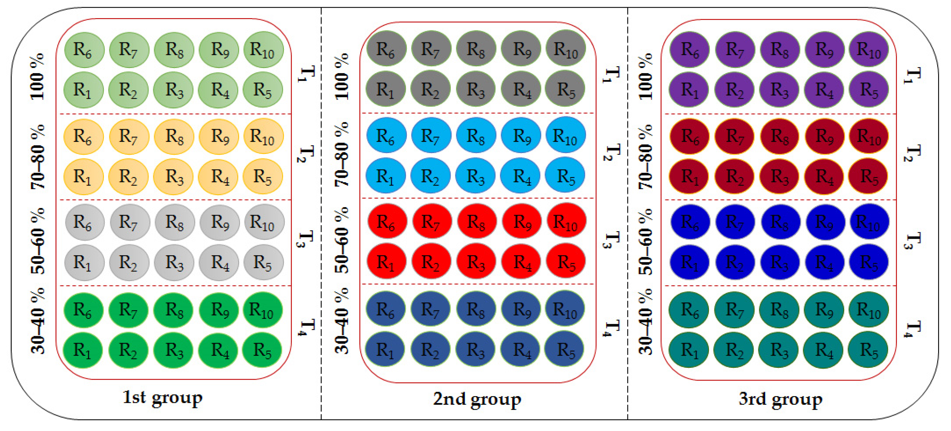
Figure 1. An experimental design layout.
Remotesensing 13 01785 g001
Figure 2. Experimental rice samples and three sections for each potted rice plant obtained by RGB camera: (a) elevation view, (b) side view, and (c) plan view.
Remotesensing 13 01785 g002
Figure 3. Raw thermal images of the rice and image segmentation with temperature distribution during four irrigation treatments: (a) 100%, (b) 80–70%, (c) 60–50%, and (d) 40–30% of field capacity at the three growth stages: tillering (1st stage), stem elongation (2nd stage), and panicle initiation (3rd stage).
Remotesensing 13 01785 g003
Figure 4. The architecture of an artificial neural network.
Remotesensing 13 01785 g004
Figure 5. Pseudo-code to train a neural network and select the top variables.
Remotesensing 13 01785 g005
Figure 6. RGB-based color features identified during neural network training loops.
Remotesensing 13 01785 g006
Figure 7. The texture features selected during neural network training loops.
Remotesensing 13 01785 g007
Figure 8. Relationship between two thermal indicators and water content of rice during the three growth stages; tillering (1st stage), stem elongation (2nd stage), and panicle initiation (3rd stage): (a) CWSI-based CWC, and (b) NRCT-based CWC.
Remotesensing 13 01785 g008
Figure 9. Learning curves of the neural network based on the best-combined variables through training, cross-validation, and testing using a different number of iterations: (a) 14VI, (b) 5GLCMF, (c) 2T, (d) VI-GLCM-T-21.
Remotesensing 13 01785 g009
Figure 10. Neural network topology with the best-combined variables: (a) 14VI, (b) 5GLCMF, (c) 2T, and (d) VI-GLCMF-T-21.
Remotesensing 13 01785 g010
Figure 11. The relationship between expected and actual CWC values employing the best-combined features: (a) VI-T-16, (b) GLCMF-T-7, and (c) VI-GLCMF-T-21.
Remotesensing 13 01785 g011
Table 1. Brief measurements of climate factors.
DateTemperature (°C)Relative Humidity (%)VPD
(Kpa)
Min.Max.Avg.Std.Min.Max.Avg.Std.
July 10 to August 122438315.2941956820.101.44
August 13 to August 30233428.54.10449770.516.971.15
August 31 to September 21183526.55.14419668.517.791.09
Where min, max, avg, and std are the values of minimum, maximum, average, and standard deviation of the measured climate factors, respectively.
Table 2. Description of different RGB imagery indices tested in this study.
RGB IndicesFormulaReferences
Normalized red index (rn)R/(R + G + B)[36]
Normalized green index (gn)G/(R + G + B)[36]
Normalized blue index (bn)B/(R + G + B)[36]
Green red ratio index (GRRI)G/R[37]
Red blue ratio index (RBRI)R/B[38]
Green blue ratio index (GBRI)G/B[38]
Normalized difference index (NDI)(rn − gn)/(rn + gn + 0.01)[39]
Green-red vegetation index (GRVI)(G − R)/(G + R)[40]
Kawashima index (IKAW)(R − B)/(R + B)[36]
Woebbecke index (WI)(G − B)/(R − G)[18]
Green leaf index (GLI)(2 × G − R − B)/(2 × G + R + B)[41]
Visible atmospherically index (VARI)(G − R)/(G + R − B)[42]
Excess red vegetation index (EXR)1.4 × rn − gn[43]
Excess blue vegetation index (EXB)1.4 × bn − gn[43]
Excess green vegetation index (EXG)2 × gn − rn − bn[43]
Excess green minus excess red index (EXGR)EXG − EXR[43]
Principal component analysis index (IPCA)0.994 × |R − B| + 0.961 × |G − B| + 0.914 × |G − R|[44]
Color index of vegetation index (CIVE)0.441 × R − 0.881 × G + 0.385 × B + 18.78745[45]
Vegetative index (VEG)G/(Ra × B(1−a)), a = 0.667[45]
Combination index (COM)0.25 × EXG + 0.3 × EXGR + 0.33 × CIVE + 0.12 × VEG[45]
Table 3. Description of the GLCMF derived from digital images.
Variable TypeFormulaReference
ContrastCon = i , j = 0 N 1 P i , j ( i j ) 2 [49]
DissimilarityDis = i , j = 0 N 1 P i , j i j
HomogeneityHom = i , j = 0 N 1 P i , j 1 + ( i j ) 2
Angular second momentASM = i , j = 0 N 1 P i , j 2
EnergyEne = ASM
CorrelationCorr = i , j = 0 N 1 P i , j   [ ( i μ i ) ( ( j μ j ) σ i σ j ]
Where Pi,j are probabilities calculated for values in GLCMF when i and j are row and column references, respectively. μ i and μ j are the mean values. σ i and σ j are the standard deviation of values. N is the number of rows or columns.
Table 4. Various architectures of the BPNN model based on VI calculated from RGB images: with MSE, RMSE, MAPE (%), Acc, and R2 in training, cross-validation, and test set.
nf(nr1,nr2)funIterMSERMSEMAPE (%)R2Acc
TrainCVTestTrainCVTestTrainCVTestTrainCVTest
20(14,10)logistic476.895.9719.3942.6252.4443.0652.8533.3043.2730.6930.6130.5560.967
19(11,13)logistic457.0176.1508.4862.6492.4802.9132.8683.3532.9480.6870.5770.5990.971
18(18,18)logistic547.5057.0467.2532.7392.6542.6933.0783.5932.8590.6650.5190.6570.971
17(2,5)logistic1409.8465.8429.7673.1382.4173.1253.6313.2773.6390.5610.6200.5380.964
16(19,5)logistic657.6896.9698.7582.7732.6392.9593.1043.5582.9790.6570.5250.5860.970
15(19,16)tanh1077.1797.0198.5122.6792.6492.9183.0023.5492.9280.6790.5580.5930.971
14 *(19,15)logistic1194.5215.2477.7762.1262.2912.7882.2443.1052.8320.7980.6250.6320.972
13(13,15)logistic706.9546.5248.7762.6372.5542.9632.8743.4563.0240.6890.5720.5850.969
12(3,3)logistic17411.2015.60911.4993.3472.3693.3913.6573.2353.5030.5000.5980.4560.964
11(11,6)logistic697.3816.8548.3972.7172.6182.8983.0143.5342.8670.6710.5510.6030.971
10(6,14)logistic637.2867.3478.4522.6992.7112.9072.9833.6633.0830.6750.5330.6000.969
9(8,15)logistic1046.7296.7228.3932.5942.5932.8972.8583.4962.8610.6990.5310.6030.971
8(14,14)logistic1096.9976.8399.5112.6452.6153.0842.9213.5493.0790.6880.5530.5500.969
7(17,14)tanh2706.7746.0689.9182.6032.4633.1492.8113.3573.2130.6980.5800.5310.968
6(7,10)logistic867.4846.3648.9832.7362.5232.9973.0693.4033.0590.6660.5650.5750.969
5(3,11)logistic2247.1496.2377.5292.6742.4972.7442.9833.3782.6300.6810.5850.6440.974
4(10,17)logistic977.6807.1568.0292.7712.6752.8343.1293.6192.7370.6570.5140.6200.973
3(6,20)tanh1507.6855.9618.2972.7722.4422.8813.0653.3112.9220.6570.6020.6070.971
2(5,15)logistic2157.3585.8199.0042.7132.4123.0012.9833.2612.8920.6720.6130.5740.971
1(8,17)logistic5119.8948.19912.3153.1452.8633.5093.4093.8793.9650.5590.4480.4170.960
Where nf is number of features, Iter is the maximum iteration of the neural network, CV is a cross-validation dataset, and * denotes best-combined VI with the lowest RMSECV.
Table 5. Various architectures of BPNN model based on GLCMF extracted from digital images with MSE, RMSE, MAPE (%), Acc, and R2 in training, cross-validation, and test set.
nf.(nr1,nr2) funIterMSERMSEMAPE (%)R2Acc
TrainCVTestTrainCVTestTrainCVTestTrainCVTest
6(16,10)relu2975.8375.5377.5992.4162.3532.7572.5823.2023.1510.7390.6120.6410.968
5 *(6,10)tanh1756.0564.6146.7942.4612.1482.6072.6072.9172.9380.7290.6560.6790.971
4(19,6)relu1416.3655.2426.3672.5232.2892.5232.7133.1242.9170.7160.6400.6990.971
3(7,13)relu1856.3395.3356.1272.5182.3092.4752.6713.1332.9490.7170.6150.7100.971
2(15,3)tanh1927.1695.03410.2492.6772.2443.2013.0263.0483.6890.6800.6440.5150.963
1(19,8)logistic6310.4427.77710.3373.2312.7893.2154.1773.9074.0670.5340.4430.5110.959
Where * refers to best-combined GLCMF at the smallest value of RMSCV.
Table 6. Various architectures of BPNN model based on thermal features with MSE, RMSE, MAPE (%), Acc, and R2 in training, cross-validation, and test set.
nf(nr1,nr2) funIterMSERMSEMAPE (%)R2Acc
TrainCVTestTrainCVTestTrainCVTestTrainCVTest
2 a(19,18)logistic2172.0081.2454.1721.4171.1162.0431.3021.4721.9890.9100.8510.8030.980
1 b(3,5)logistic2979.5296.49710.4733.0872.5493.2393.4243.4593.7820.5750.5660.5050.962
Where a is the best-combined variables of CWSI-NRCT, and b is the indicator of CWSI.
Table 7. Various architectures of BPNN model depending on the best-combined features extracted from visible and thermal imagery, with MSE, RMSE, MAPE (%), Acc, and R2 in training, cross-validation, and test set.
nf(nr1,nr2) fun.IterMSERMSEMAPE (%)R2AccC.T.
TrainCVTestTrainCVTestTrainCVTestTrainCVTest
7 a(18,9)logistic2750.1190.1990.5830.3460.4470.7640.3660.5990.6680.9950.9820.9720.99328.158
16 b(7,12)logistic1300.3550.4370.4550.5960.6610.6740.6040.8910.6820.9840.9560.9780.99329.977
21 c(8,9)logistic4220.0630.1300.3590.2510.3610.5990.2510.4800.5640.9970.9840.9830.99431.911
Where a is 5 GLCMF and 2 T, b is 14 VI and 2 T, c is 14 VI and 5 GLCMF and 2 T, and C.T. is the consumption time required to analyze the data across a single sample to predict the CWC (sec).
Publisher’s Note: MDPI stays neutral with regard to jurisdictional claims in published maps and institutional affiliations.