
Single Image Super-Resolution Restoration of TGO CaSSIS Colour Images: Demonstration with Perseverance Rover Landing Site and Mars Science Targets

 ,
, 
 , ,
, ,
Abstract
1. Introduction
1.1. Study Sites
1.2. Previous Work
2. Materials and Methods
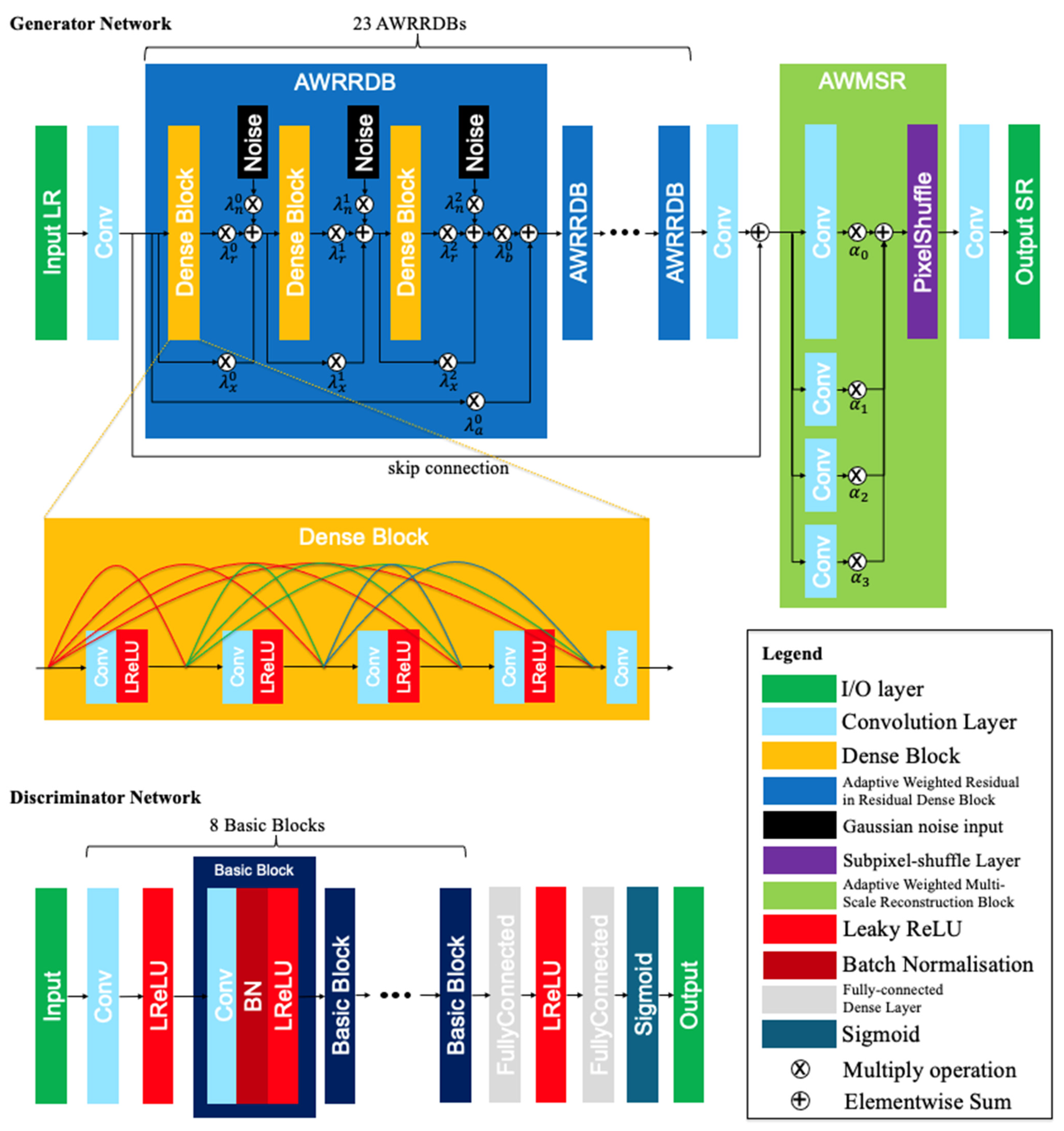
2.1. MARSGAN Architecture
2.2. Loss Functions
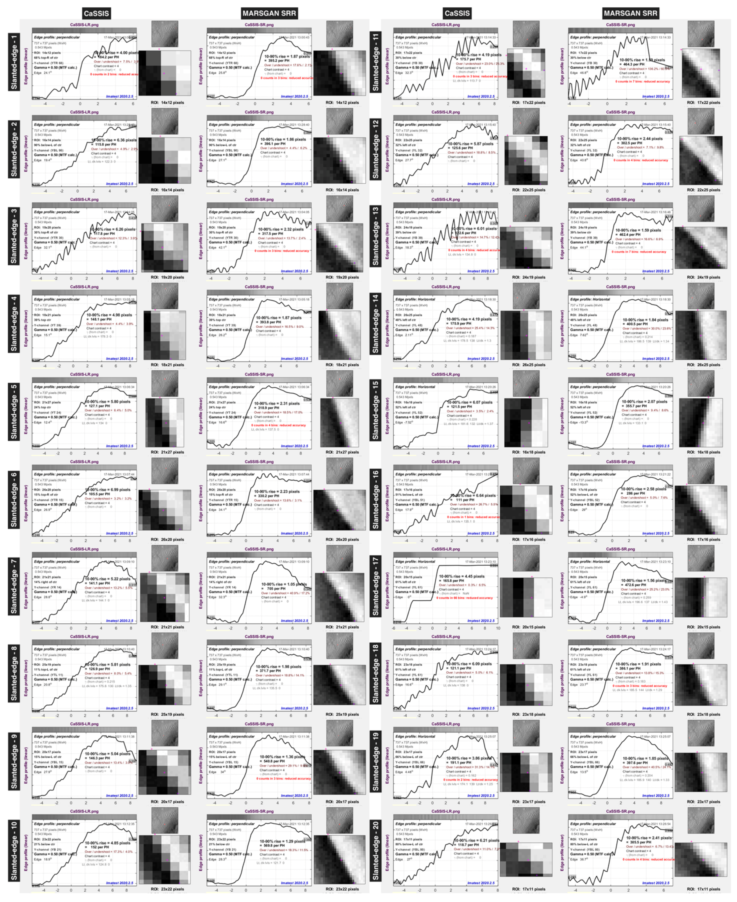
2.3. Assessment Methods
- (1)
- PSNR: PSNR is derived from the MSE and indicates the ratio of the maximum pixel intensity to the power of the distortion. A mathematical expression of PSNR can formulated aswhere denotes the target image (the CaSSIS SRR image in our case), denotes the reference image (the down-sampled HiRISE image in our case), and PeakVal is the maximum value of the reference image (normalised to 255 for 8-bit image in our case).
- (2)
- MSSIM [97]. MSSIM is the mean of locally computed structural similarity. The structural similarity index is derived using patterns of pixel intensities among neighbouring pixels with normalised brightness and contrast. MSSIM can be formulated aswhere E represents the operation of mean, , , , , and are the local means, standard deviations, and cross-covariance of the target image and reference image respectively. and are constants based on the dynamic range of pixel values.
- (3)
- BRISQUE [98]. The BRISQUE model provides subjective quality scores based on a pre-trained model using images with known distortions. The score range is [0,100] and lower values reflect better perceptual quality.
- (4)
- PIQE [99]. PIQE measures the quality of images using block-wise calculation against arbitrary distortions. The score range is [0,100] and lower values reflect better perceptual quality.
2.4. Training and Testing
3. Results
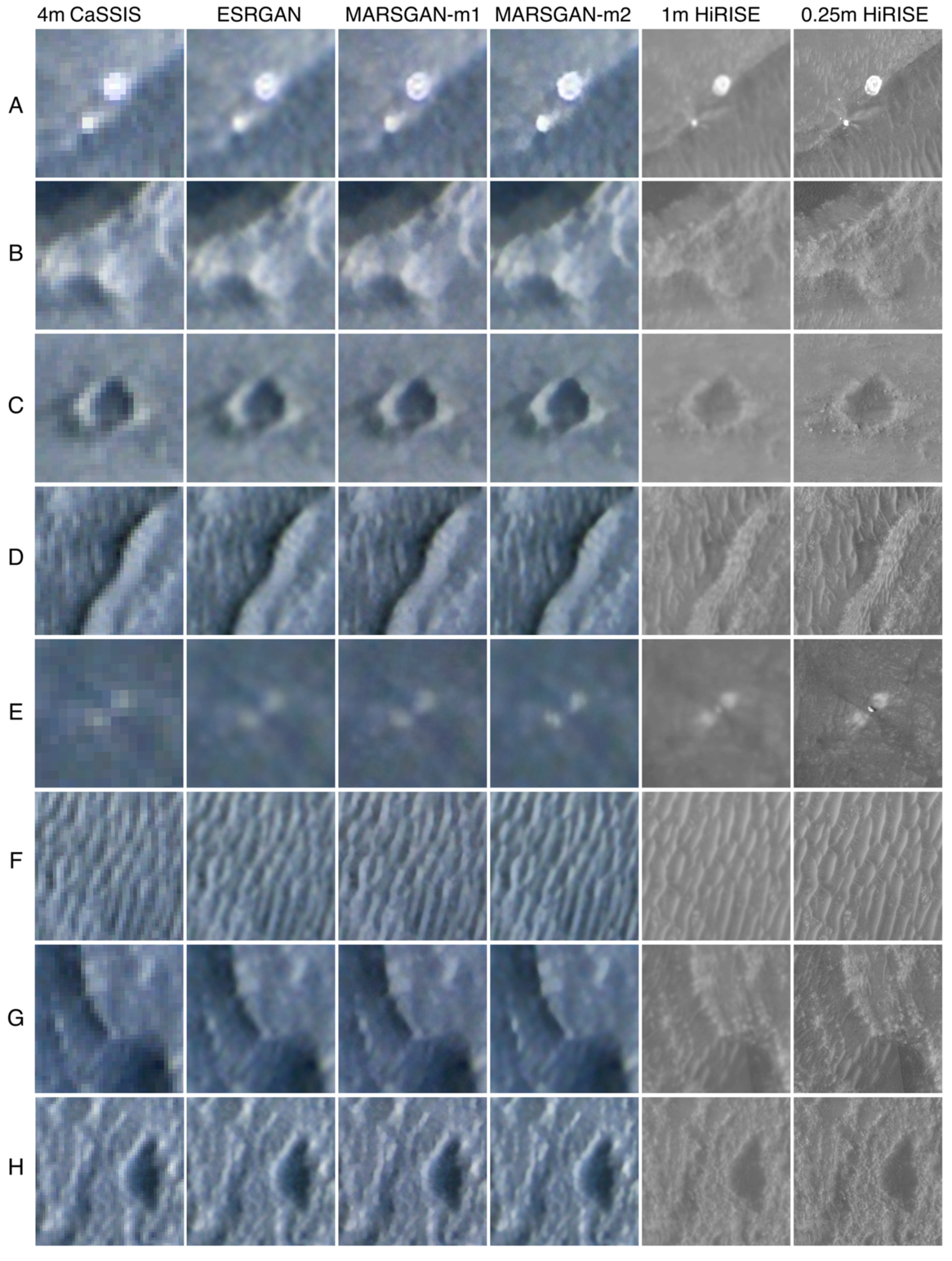
3.1. Results and Assessment for Jezero Crater
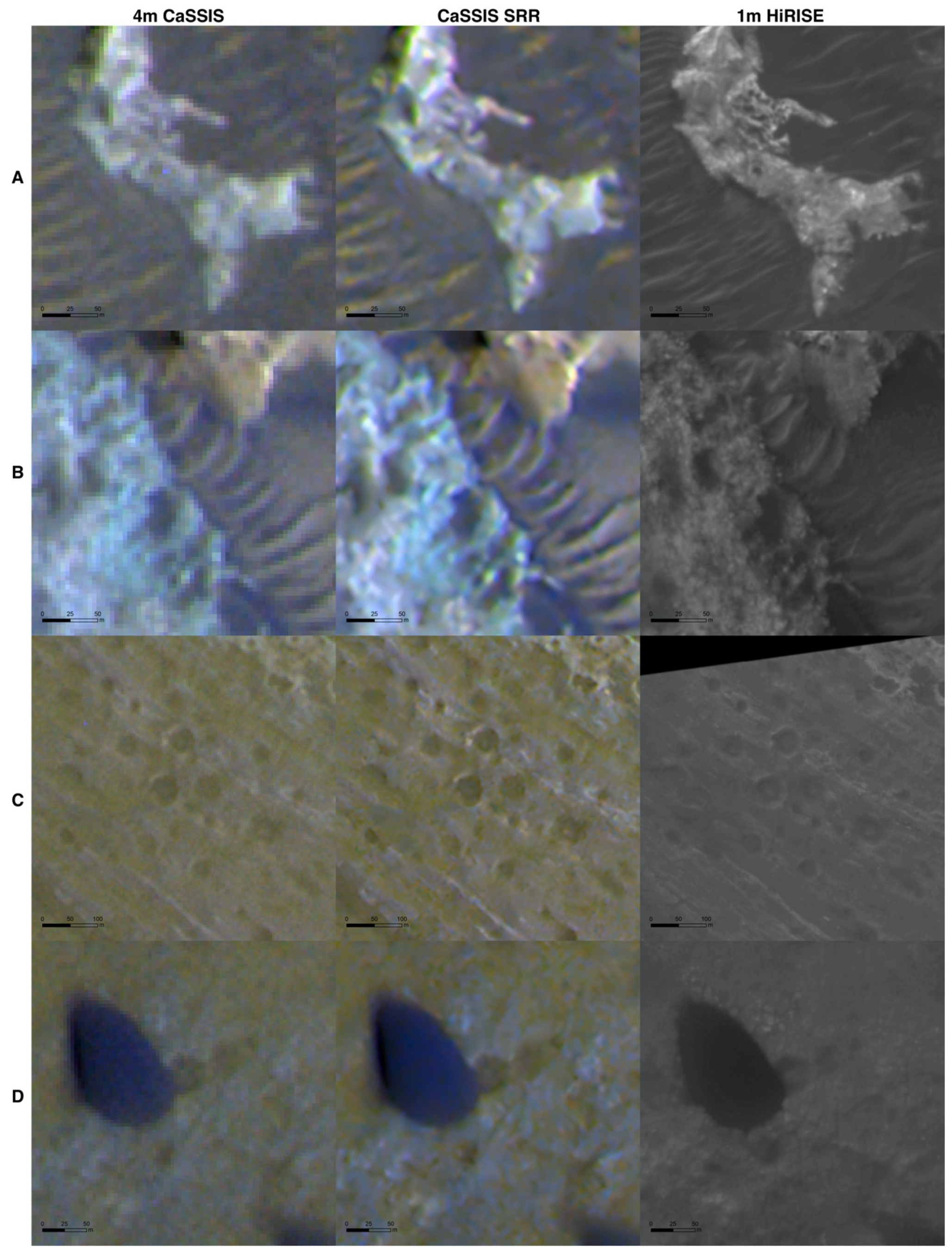
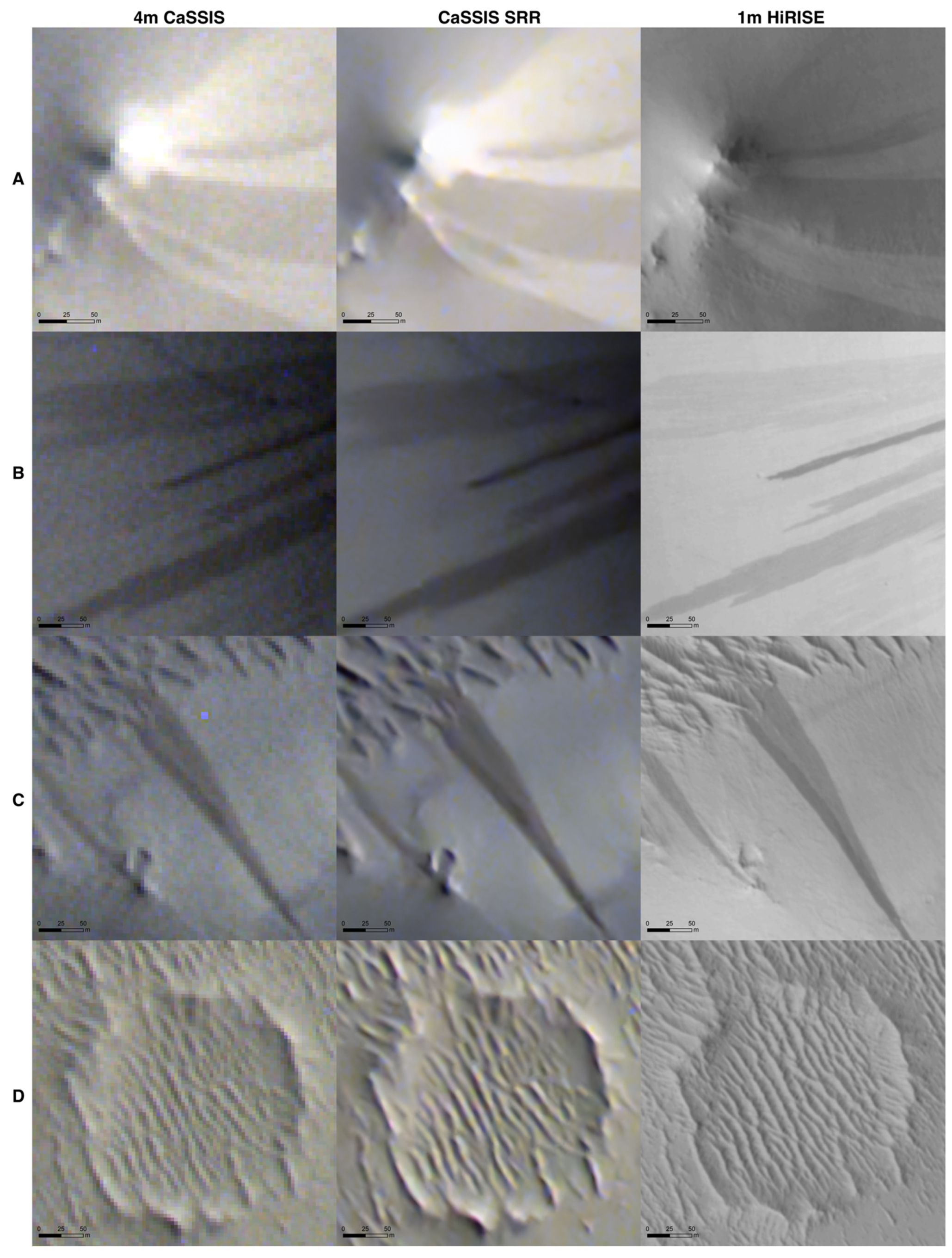
3.2. Results and Visual Demonstration of Science Targets/Sites
4. Discussion
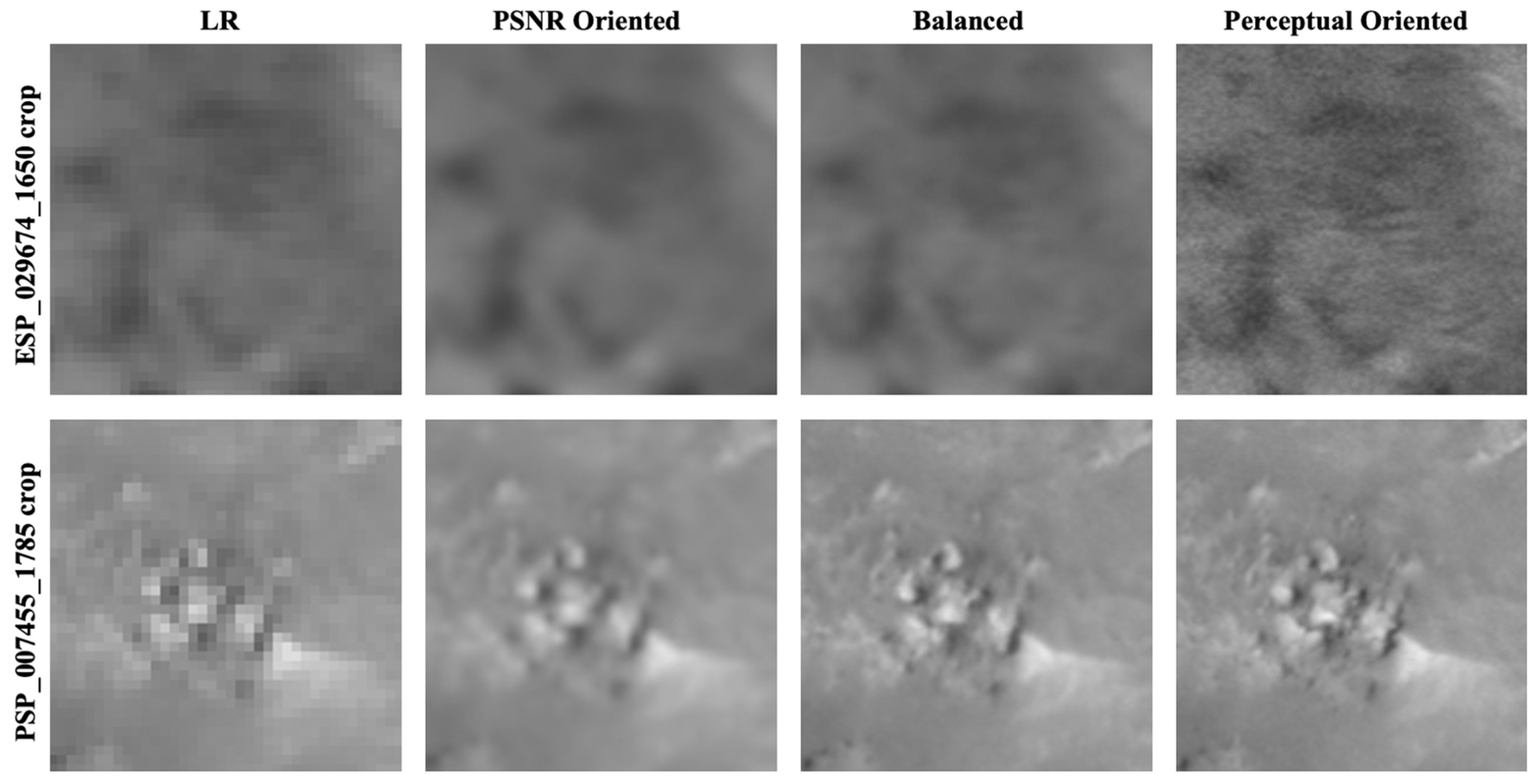
4.1. Perceptual-Driven Solution or PSNR-Driven Solution
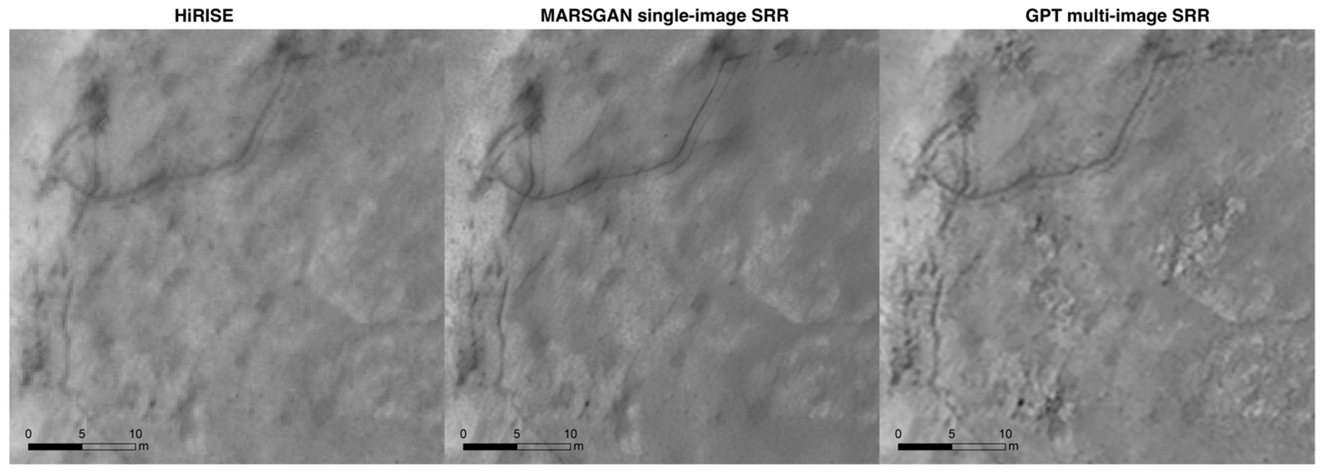
4.2. Single Image SRR or Multi-Image SRR
4.3. Extendability with Other Datasets
5. Conclusions
Supplementary Materials
Author Contributions
Funding
Institutional Review Board Statement
Informed Consent Statement
Data Availability Statement
Acknowledgments
Conflicts of Interest
References
- Thomas, N.; Cremonese, G.; Ziethe, R.; Gerber, M.; Brändli, M.; Bruno, G.; Erismann, M.; Gambicorti, L.; Gerber, T.; Ghose, K.; et al. The colour and stereo surface imaging system (CaSSIS) for the ExoMars trace gas orbiter. Space Sci. Rev. 2017, 212, 1897–1944. [Google Scholar] [CrossRef]
- Malin, M.C.; Bell, J.F.; Cantor, B.A.; Caplinger, M.A.; Calvin, W.M.; Clancy, R.T.; Edgett, K.S.; Edwards, L.; Haberle, R.M.; James, P.B.; et al. Context camera investigation on board the Mars Reconnaissance Orbiter. J. Geophys. Res. Space Phys. 2007, 112, 112. [Google Scholar] [CrossRef]
- McEwen, A.S.; Eliason, E.M.; Bergstrom, J.W.; Bridges, N.T.; Hansen, C.J.; Delamere, W.A.; Grant, J.A.; Gulick, V.C.; Herkenhoff, K.E.; Keszthelyi, L.; et al. Mars reconnaissance orbiter’s high resolution imaging science experiment (HiRISE). J. Geophys. Res. Space Phys. 2007, 112. [Google Scholar] [CrossRef]
- Tao, Y.; Muller, J.-P. A novel method for surface exploration: Super-resolution restoration of Mars repeat-pass orbital imagery. Planet. Space Sci. 2016, 121, 103–114. [Google Scholar] [CrossRef]
- Bridges, J.C.; Clemmet, J.; Croon, M.; Sims, M.R.; Pullan, D.; Muller, J.P.; Tao, Y.; Xiong, S.; Putri, A.R.; Parker, T.; et al. Identification of the Beagle 2 lander on Mars. R. Soc. Open Sci. 2017, 4, 170785. [Google Scholar] [CrossRef]
- Grant, J.A.; Golombek, M.P.; Wilson, S.A.; Farley, K.A.; Williford, K.H.; Chen, A. The science process for selecting the landing site for the 2020 Mars rover. Planet. Space Sci. 2018, 164, 106–126. [Google Scholar] [CrossRef]
- Stack, K.M.; Williams, N.R.; Calef, F.; Sun, V.Z.; Williford, K.H.; Farley, K.A.; Eide, S.; Flannery, D.; Hughes, C.; Jacob, S.R.; et al. Photogeologic map of the perseverance rover field site in Jezero Crater constructed by the Mars 2020 Science Team. Space Sci. Rev. 2020, 216, 1–47. [Google Scholar] [CrossRef]
- Ehlmann, B.L.; Mustard, J.F.; Fassett, C.I.; Schon, S.C.; Head, J.W., III; Des Marais, D.J.; Grant, J.A.; Murchie, S.L. Clay minerals in delta deposits and organic preservation potential on Mars. Nat. Geosci. 2008, 1, 355–358. [Google Scholar] [CrossRef]
- Wray, J.J.; Murchie, S.L.; Squyres, S.W.; Seelos, F.P.; Tornabene, L.L. Diverse aqueous environments on ancient Mars revealed in the southern highlands. Geology 2009, 37, 1043–1046. [Google Scholar] [CrossRef]
- Breed, C.S.; Grolier, M.J.; McCauley, J.F. Morphology and distribution of common ‘sand’ dunes on Mars: Comparison with the Earth. J. Geophys. Res. Solid Earth 1979, 84, 8183–8204. [Google Scholar] [CrossRef]
- Bishop, M.A. Dark dunes of Mars: An orbit-to-ground multidisciplinary perspective of aeolian science. In Dynamic Mars; Elsevier: Amsterdam, The Netherlands, 2018; pp. 317–360. [Google Scholar]
- Hayward, R.K.; Mullins, K.F.; Fenton, L.K.; Hare, T.M.; Titus, T.N.; Bourke, M.C.; Colaprete, A.; Christensen, P.R. Mars global digital dune database and initial science results. J. Geophys. Res. Space Phys. 2007, 112. [Google Scholar] [CrossRef]
- Balme, M.; Berman, D.C.; Bourke, M.C.; Zimbelman, J.R. Transverse aeolian ridges (TARs) on Mars. Geomorphology 2008, 101, 703–720. [Google Scholar] [CrossRef]
- Zimbelman, J.R. Transverse aeolian ridges on Mars: First results from HiRISE images. Geomorphology 2010, 121, 22–29. [Google Scholar] [CrossRef]
- Baker, M.M.; Lapotre, M.G.; Minitti, M.E.; Newman, C.E.; Sullivan, R.; Weitz, C.M.; Rubin, D.M.; Vasavada, A.R.; Bridges, N.T.; Lewis, K.W. The Bagnold Dunes in southern summer: Active sediment transport on Mars observed by the Curiosity rover. Geophys. Res. Lett. 2018, 45, 8853–8863. [Google Scholar] [CrossRef]
- Silvestro, S.; Fenton, L.K.; Vaz, D.A.; Bridges, N.T.; Ori, G.G. Ripple migration and dune activity on Mars: Evidence for dynamic wind processes. Geophys. Res. Lett. 2010, 37. [Google Scholar] [CrossRef]
- Hansen, C.J.; Bourke, M.; Bridges, N.T.; Byrne, S.; Colon, C.; Diniega, S.; Dundas, C.; Herkenhoff, K.; McEwen, A.; Mellon, M.; et al. Seasonal erosion and restoration of Mars’ northern polar dunes. Science 2011, 331, 575–578. [Google Scholar] [CrossRef] [PubMed]
- Chojnacki, M.; Burr, D.M.; Moersch, J.E.; Michaels, T.I. Orbital observations of contemporary dune activity in Endeavor crater, Meridiani Planum, Mars. J. Geophys. Res. Space Phys. 2011, 116. [Google Scholar] [CrossRef]
- Berman, D.C.; Balme, M.R.; Michalski, J.R.; Clark, S.C.; Joseph, E.C. High-resolution investigations of transverse aeolian ridges on Mars. Icarus 2018, 312, 247–266. [Google Scholar] [CrossRef]
- Geissler, P.E. The birth and death of transverse aeolian ridges on Mars. J. Geophys. Res. Planets 2014, 119, 2583–2599. [Google Scholar] [CrossRef]
- Schorghofer, N.; Aharonson, O.; Gerstell, M.F.; Tatsumi, L. Three decades of slope streak activity on Mars. Icarus 2007, 191, 132–140. [Google Scholar] [CrossRef]
- Sullivan, R.; Thomas, P.; Veverka, J.; Malin, M.; Edgett, K.S. Mass movement slope streaks imaged by the Mars Orbiter Camera. J. Geophys. Res. Space Phys. 2001, 106, 23607–23633. [Google Scholar] [CrossRef]
- Aharonson, O.; Schorghofer, N.; Gerstell, M.F. Slope streak formation and dust deposition rates on Mars. J. Geophys. Res. Space Phys. 2003, 108. [Google Scholar] [CrossRef]
- Schorghofer, N.; King, C.M. Sporadic formation of slope streaks on Mars. Icarus 2011, 216, 159–168. [Google Scholar] [CrossRef]
- Heyer, T.; Kreslavsky, M.; Hiesinger, H.; Reiss, D.; Bernhardt, H.; Jaumann, R. Seasonal formation rates of martian slope streaks. Icarus 2019, 323, 76–86. [Google Scholar] [CrossRef]
- Bhardwaj, A.; Sam, L.; Martín-Torres, F.J.; Zorzano, M.P. Are Slope Streaks Indicative of Global-Scale Aqueous Processes on Contemporary Mars? Rev. Geophys. 2019, 57, 48–77. [Google Scholar] [CrossRef]
- Heyer, T.; Raack, J.; Hiesinger, H.; Jaumann, R. Dust devil triggering of slope streaks on Mars. Icarus 2020, 351, 113951. [Google Scholar] [CrossRef]
- Ferris, J.C.; Dohm, J.M.; Baker, V.R.; Maddock III, T. Dark slope streaks on Mars: Are aqueous processes involved? Geophys. Res. Lett. 2002, 29, 128-1–128-4. [Google Scholar] [CrossRef]
- Diniega, S.; Byrne, S.; Bridges, N.T.; Dundas, C.M.; McEwen, A.S. Seasonality of present-day Martian dune-gully activity. Geology 2010, 38, 1047–1050. [Google Scholar] [CrossRef]
- Pasquon, K.; Gargani, J.; Nachon, M.; Conway, S.J.; Massé, M.; Jouannic, G.; Balme, M.R.; Costard, F.; Vincendon, M. Are different Martian gully morphologies due to different processes on the Kaiser dune field? Geol. Soc. Lond. Spec. Publ. 2019, 467, 145–164. [Google Scholar] [CrossRef]
- Pasquon, K.; Gargani, J.; Massé, M.; Vincendon, M.; Conway, S.J.; Séjourné, A.; Jomelli, V.; Balme, M.R.; Lopez, S.; Guimpier, A. Present-day development of gully-channel sinuosity by carbon dioxide gas supported flows on Mars. Icarus 2019, 329, 296–313. [Google Scholar] [CrossRef]
- Gardin, E.; Allemand, P.; Quantin, C.; Thollot, P. Defrosting, dark flow features, and dune activity on Mars: Example in Russell crater. J. Geophys. Res. Space Phys. 2010, 115. [Google Scholar] [CrossRef]
- Kossacki, K.J.; Leliwa-Kopystyński, J. Non-uniform seasonal defrosting of subpolar dune field on Mars. Icarus 2004, 168, 201–204. [Google Scholar] [CrossRef]
- Hansen, C.J.; Byrne, S.; Portyankina, G.; Bourke, M.; Dundas, C.; McEwen, A.; Mellon, M.; Pommerol, A.; Thomas, N. Observations of the northern seasonal polar cap on Mars: I. Spring sublimation activity and processes. Icarus 2013, 225, 881–897. [Google Scholar] [CrossRef]
- Kieffer, H.H.; Christensen, P.R.; Titus, T.N. CO 2 jets formed by sublimation beneath translucent slab ice in Mars’ seasonal south polar ice cap. Nature 2006, 442, 793–796. [Google Scholar] [CrossRef] [PubMed]
- Dundas, C.M.; McEwen, A.S.; Diniega, S.; Hansen, C.J.; Byrne, S.; McElwaine, J.N. The formation of gullies on Mars today. Geol. Soc. Lond. Spec. Publ. 2019, 467, 67–94. [Google Scholar] [CrossRef]
- Dundas, C.M.; Diniega, S.; Hansen, C.J.; Byrne, S.; McEwen, A.S. Seasonal activity and morphological changes in Martian gullies. Icarus 2012, 220, 124–143. [Google Scholar] [CrossRef]
- Dundas, C.M.; McEwen, A.S.; Diniega, S.; Byrne, S.; Martinez-Alonso, S. New and recent gully activity on Mars as seen by HiRISE. Geophys. Res. Lett. 2010, 37, 37. [Google Scholar] [CrossRef]
- Dundas, C.M.; Diniega, S.; McEwen, A.S. Long-term monitoring of Martian gully formation and evolution with MRO/HiRISE. Icarus 2015, 251, 244–263. [Google Scholar] [CrossRef]
- Tornabene, L.L.; Osinski, G.R.; McEwen, A.S.; Boyce, J.M.; Bray, V.J.; Caudill, C.M.; Grant, J.A.; Hamilton, C.W.; Mattson, S.S.; Mouginis-Mark, P.J. Widespread crater-related pitted materials on Mars: Further evidence for the role of target volatiles during the impact process. Icarus 2012, 220, 348–368. [Google Scholar] [CrossRef]
- Boyce, J.M.; Wilson, L.; Mouginis-Mark, P.J.; Hamilton, C.W.; Tornabene, L.L. Origin of small pits in martian impact craters. Icarus 2012, 221, 262–275. [Google Scholar] [CrossRef]
- McEwen, A.S.; Ojha, L.; Dundas, C.M.; Mattson, S.S.; Byrne, S.; Wray, J.J.; Cull, S.C.; Murchie, S.L.; Thomas, N.; Gulick, V.C. Seasonal flows on warm Martian slopes. Science 2011, 333, 740–743. [Google Scholar] [CrossRef]
- Ojha, L.; McEwen, A.; Dundas, C.; Byrne, S.; Mattson, S.; Wray, J.; Masse, M.; Schaefer, E. HiRISE observations of recurring slope lineae (RSL) during southern summer on Mars. Icarus 2014, 231, 365–376. [Google Scholar] [CrossRef]
- Munaretto, G.; Pajola, M.; Cremonese, G.; Re, C.; Lucchetti, A.; Simioni, E.; McEwen, A.; Pommerol, A.; Becerra, P.; Conway, S.; et al. Implications for the origin and evolution of Martian Recurring Slope Lineae at Hale crater from CaSSIS observations. Planet. Space Sci. 2020, 187, 104947. [Google Scholar] [CrossRef]
- Stillman, D.E.; Michaels, T.I.; Grimm, R.E.; Harrison, K.P. New observations of martian southern mid-latitude recurring slope lineae (RSL) imply formation by freshwater subsurface flows. Icarus 2014, 233, 328–341. [Google Scholar] [CrossRef]
- Stillman, D.E.; Grimm, R.E. Two pulses of seasonal activity in martian southern mid-latitude recurring slope lineae (RSL). Icarus 2018, 302, 126–133. [Google Scholar] [CrossRef]
- McEwen, A.S.; Schaefer, E.I.; Dundas, C.M.; Sutton, S.S.; Tamppari, L.K.; Chojnacki, M. Mars: Abundant Recurring Slope Lineae (RSL) Following the Planet-Encircling Dust Event (PEDE) of 2018. J. Geophys. Res. Planets 2020. [Google Scholar] [CrossRef]
- Gough, R.V.; Nuding, D.L.; Archer Jr, P.D.; Fernanders, M.S.; Guzewich, S.D.; Tolbert, M.A.; Toigo, A.D. Changes in Soil Cohesion Due to Water Vapor Exchange: A Proposed Dry-Flow Trigger Mechanism for Recurring Slope Lineae on Mars. Geophy. Res. Lett. 2020, 47. [Google Scholar] [CrossRef]
- Vincendon, M.; Pilorget, C.; Carter, J.; Stcherbinine, A. Observational evidence for a dry dust-wind origin of Mars seasonal dark flows. Icarus 2019, 325, 115–127. [Google Scholar] [CrossRef]
- Ojha, L.; Wilhelm, M.B.; Murchie, S.L.; McEwen, A.S.; Wray, J.J.; Hanley, J.; Massé, M.; Chojnacki, M. Spectral evidence for hydrated salts in recurring slope lineae on Mars. Nat. Geosci. 2015, 8, 829–832. [Google Scholar] [CrossRef]
- Jones, A.P.; McEwen, A.S.; Tornabene, L.L.; Baker, V.R.; Melosh, H.J.; Berman, D.C. A geomorphic analysis of Hale crater, Mars: The effects of impact into ice-rich crust. Icarus 2011, 211, 259–272. [Google Scholar] [CrossRef]
- El-Maarry, M.R.; Dohm, J.M.; Michael, G.; Thomas, N.; Maruyama, S. Morphology and evolution of the ejecta of Hale crater in Argyre basin, Mars: Results from high resolution mapping. Icarus 2013, 226, 905–922. [Google Scholar] [CrossRef]
- Collins-May, J.L.; Carr, J.R.; Balme, M.R.; Ross, N.; Russell, A.J.; Brough, S.; Gallagher, C. Postimpact Evolution of the Southern Hale Crater Ejecta, Mars. J. Geophys. Res. Planets 2020, 125, 6302. [Google Scholar] [CrossRef]
- Séjourné, A.; Costard, F.; Gargani, J.; Soare, R.J.; Fedorov, A.; Marmo, C. Scalloped depressions and small-sized polygons in western Utopia Planitia, Mars: A new formation hypothesis. Planet. Space Sci. 2011, 59, 412–422. [Google Scholar] [CrossRef]
- Lefort, A.; Russell, P.S.; Thomas, N. Scalloped terrains in the Peneus and Amphitrites Paterae region of Mars as observed by HiRISE. Icarus 2010, 205, 259–268. [Google Scholar] [CrossRef]
- Zanetti, M.; Hiesinger, H.; Reiss, D.; Hauber, E.; Neukum, G. Distribution and evolution of scalloped terrain in the southern hemisphere, Mars. Icarus 2010, 206, 691–706. [Google Scholar] [CrossRef]
- Dundas, C.M. Effects of varying obliquity on Martian sublimation thermokarst landforms. Icarus 2017, 281, 115–120. [Google Scholar] [CrossRef]
- Soare, R.J.; Conway, S.J.; Gallagher, C.; Dohm, J.M. Ice-rich (periglacial) vs icy (glacial) depressions in the Argyre region, Mars: A proposed cold-climate dichotomy of landforms. Icarus 2017, 282, 70–83. [Google Scholar] [CrossRef]
- Thomas, P.; Gierasch, P.J. Dust devils on Mars. Science 1985, 230, 175–177. [Google Scholar] [CrossRef]
- Balme, M.; Greeley, R. Dust devils on Earth and Mars. Rev. Geophys. 2006, 44. [Google Scholar] [CrossRef]
- Whelley, P.L.; Greeley, R. The distribution of dust devil activity on Mars. J. Geophys. Res. Space Phys. 2008, 113. [Google Scholar] [CrossRef]
- Reiss, D.; Fenton, L.; Neakrase, L.; Zimmerman, M.; Statella, T.; Whelley, P.; Rossi, A.P.; Balme, M. Dust devil tracks. Space Sci. Rev. 2016, 203, 143–181. [Google Scholar] [CrossRef]
- Forsberg-Taylor, N.K.; Howard, A.D.; Craddock, R.A. Crater degradation in the Martian highlands: Morphometric analysis of the Sinus Sabaeus region and simulation modeling suggest fluvial processes. J. Geophys. Res. Space Phys. 2004, 109. [Google Scholar] [CrossRef]
- Craddock, R.A.; Maxwell, T.A. Geomorphic evolution of the Martian highlands through ancient fluvial processes. J. Geophys. Res. Space Phys. 1993, 98, 3453–3468. [Google Scholar] [CrossRef]
- Piqueux, S.; Byrne, S.; Richardson, M.I. Sublimation of Mars’s southern seasonal CO2 ice cap and the formation of spiders. J. Geophys. Res. Phys. Planets 2003, 108. [Google Scholar] [CrossRef]
- Hao, J.; Michael, G.G.; Adeli, S.; Jaumann, R. Araneiform terrain formation in Angustus Labyrinthus, Mars. Icarus 2019, 317, 479–490. [Google Scholar] [CrossRef]
- Thomas, N.; Portyankina, G.; Hansen, C.J.; Pommerol, A. HiRISE observations of gas sublimation-driven activity in Mars’ southern polar regions: IV. Fluid dynamics models of CO2 jets. Icarus 2011, 212, 66–85. [Google Scholar] [CrossRef]
- Hansen, C.J.; Thomas, N.; Portyankina, G.; McEwen, A.; Becker, T.; Byrne, S.; Herkenhoff, K.; Kieffer, H.; Mellon, M. HiRISE observations of gas sublimation-driven activity in Mars’ southern polar regions: I. Erosion of the surface. Icarus 2010, 205, 283–295. [Google Scholar] [CrossRef]
- Portyankina, G.; Markiewicz, W.J.; Thomas, N.; Hansen, C.J.; Milazzo, M. HiRISE observations of gas sublimation-driven activity in Mars’ southern polar regions: III. Models of processes involving translucent ice. Icarus 2010, 205, 311–320. [Google Scholar] [CrossRef]
- Tsai, R.Y.; Huang, T.S. Multipleframe Image Restoration and Registration. In Advances in Computer Vision and Image Processing; JAI Press Inc.: New York, NY, USA, 1984; pp. 317–339. [Google Scholar]
- Keren, D.; Peleg, S.; Brada, R. Image sequence enhancement using subpixel displacements. In Proceedings of the IEEE Conference on Computer Vision and Pattern Recognition, Ann Arbor, MI, USA, 5–9 June 1988; pp. 742–746. [Google Scholar]
- Hardie, R.C.; Barnard, K.J.; Armstrong, E.E. Joint MAP registration and high resolution image estimation using a sequence of undersampled images. IEEE Trans. Image Process. 1997, 6, 1621–1633. [Google Scholar] [CrossRef]
- Farsiu, S.; Robinson, D.; Elad, M.; Milanfar, P. Fast and robust multi-frame super-resolution. IEEE Trans. Image Process. 2004, 13, 1327–1344. [Google Scholar] [CrossRef]
- Yuan, Q.; Zhang, L.; Shen, H. Multiframe super-resolution employing a spatially weighted total variation model. IEEE Trans. Circuits Syst. Video Technol. 2012, 22, 379–392. [Google Scholar] [CrossRef]
- Tao, Y.; Muller, J.-P. Super-resolution restoration of MISR images using the UCL MAGiGAN system. Remote Sens. 2019, 11, 52. [Google Scholar] [CrossRef]
- Dong, C.; Loy, C.C.; He, K.; Tang, X. Learning a deep convolutional network for image super-resolution. In Proceedings of the ECCV 2014, Zurich, Switzerland, 6–12 September 2014; pp. 184–199. [Google Scholar]
- Kim, J.; Kwon Lee, J.; Mu Lee, K. Accurate image super-resolution using very deep convolutional networks. In Proceedings of the IEEE conference on computer vision and pattern recognition, Las Vegas, NV, USA, 27–30 June 2016; pp. 1646–1654. [Google Scholar]
- Simonyan, K.; Zisserman, A. Very deep convolutional networks for large-scale image recognition. In International Conference on Learning Representations (ICLR). arXiv 2014, arXiv:1409.1556. [Google Scholar]
- Dong, C.; Loy, C.C.; Tang, X. Accelerating the super-resolution convolutional neural network. In Transactions on Petri Nets and Other Models of Concurrency XV; Springer: Cham, Switzerland, 2016; pp. 391–407. [Google Scholar]
- Shi, W.; Caballero, J.; Huszár, F.; Totz, J.; Aitken, A.P.; Bishop, R.; Rueckert, D.; Wang, Z. Real-time single image and video super-resolution using an efficient sub-pixel convolutional neural network. In Proceedings of the IEEE conference on computer vision and pattern recognition, Las Vegas, NV, USA, 27–30 June 2016; pp. 1874–1883. [Google Scholar]
- Lim, B.; Son, S.; Kim, H.; Nah, S.; Lee, K.M. Enhanced deep residual networks for single image super-resolution. In Proceedings of the IEEE conference on computer vision and pattern recognition workshops, Honolulu, HI, USA, 21–26 July 2017; pp. 136–144. [Google Scholar]
- Yu, J.; Fan, Y.; Yang, J.; Xu, N.; Wang, Z.; Wang, X.; Huang, T. Wide activation for efficient and accurate image super-resolution. arXiv 2018, arXiv:1808.08718. [Google Scholar]
- Ahn, N.; Kang, B.; Sohn, K.A. Fast, accurate, and lightweight super-resolution with cascading residual network. In Proceedings of the European Conference on Computer Vision (ECCV), Munich, Germany, 8–14 September 2018; pp. 252–268. [Google Scholar]
- He, K.; Zhang, X.; Ren, S.; Sun, J. Deep residual learning for image recognition. In Proceedings of the IEEE conference on computer vision and pattern recognition, Amsterdam, The Netherlands, 11–14 October 2016; pp. 770–778. [Google Scholar]
- Ledig, C.; Theis, L.; Huszár, F.; Caballero, J.; Cunningham, A.; Acosta, A.; Aitken, A.; Tejani, A.; Totz, J.; Wang, Z.; et al. Photo-realistic single image super-resolution using a generative adversarial network. In Proceedings of the IEEE conference on computer vision and pattern recognition, Honolulu, HI, USA, 21–26 July 2017; pp. 4681–4690. [Google Scholar]
- Kim, J.; Lee, J.K.; Lee, K.M. Deeply-recursive convolutional network for image super-resolution. In Proceedings of the IEEE conference on computer vision and pattern recognition, Amsterdam, The Netherlands, 11–14 October 2016; pp. 1637–1645. [Google Scholar]
- Tai, Y.; Yang, J.; Liu, X. Image super-resolution via deep recursive residual network. In Proceedings of the IEEE conference on computer vision and pattern recognition, Honolulu, HI, USA, 21–26 July 2017; pp. 3147–3155. [Google Scholar]
- Wang, C.; Li, Z.; Shi, J. Lightweight image super-resolution with adaptive weighted learning network. arXiv 2019, arXiv:1904.02358. [Google Scholar]
- Zhang, Y.; Li, K.; Li, K.; Wang, L.; Zhong, B.; Fu, Y. Image super-resolution using very deep residual channel attention networks. In Proceedings of the European conference on computer vision (ECCV), Munich, Germany, 8–14 September 2018; pp. 286–301. [Google Scholar]
- Goodfellow, I.J.; Pouget-Abadie, J.; Mirza, M.; Xu, B.; Warde-Farley, D.; Ozair, S.; Courville, A.; Bengio, Y. Generative adversarial networks. arXiv 2014, arXiv:1406.2661. [Google Scholar] [CrossRef]
- Sajjadi, M.S.; Scholkopf, B.; Hirsch, M. EnhanceNet: Single image super-resolution through automated texture synthesis. In Proceedings of the IEEE International Conference on Computer Vision, Venice, Italy, 22–29 October 2017; pp. 4491–4500. [Google Scholar]
- Wang, X.; Yu, K.; Wu, S.; Gu, J.; Liu, Y.; Dong, C.; Qiao, Y.; Loy, C.C. ESRGAN: Enhanced super-resolution generative adversarial networks. In Proceedings of the European Conference on Computer Vision (ECCV) Workshops, Munich, Germany, 8–14 September 2018. [Google Scholar]
- Rakotonirina, N.C.; Rasoanaivo, A. ESRGAN+: Further improving enhanced super-resolution generative adversarial network. In Proceedings of the ICASSP 2020-2020 IEEE International Conference on Acoustics, Speech and Signal Processing (ICASSP), Barcelona, Spain, 4–8 May 2020; pp. 3637–3641. [Google Scholar]
- Zhang, W.; Liu, Y.; Dong, C.; Qiao, Y. RankSRGAN: Generative adversarial networks with ranker for image super-resolution. In Proceedings of the IEEE/CVF International Conference on Computer Vision, Seoul, Korea, 27–28 October 2019; pp. 3096–3105. [Google Scholar]
- Jolicoeur-Martineau, A. The relativistic discriminator: A key element missing from standard GAN. arXiv 2018, arXiv:1807.00734. [Google Scholar]
- Tao, Y.; Muller, J.-P.; Poole, W. Automated localisation of Mars rovers using co-registered HiRISE-CTX-HRSC orthorectified images and wide baseline Navcam orthorectified mosaics. Icarus 2016, 280, 139–157. [Google Scholar] [CrossRef]
- Zhou, W.; Bovik, A.C.; Sheikh, H.R.; Simoncelli, E.P. Image Qualifty Assessment: From Error Visibility to Structural Similarity. IEEE Trans. Image Process. 2004, 13, 600–612. [Google Scholar]
- Mittal, A.; Moorthy, A.K.; Bovik, A.C. No-Reference Image Quality Assessment in the Spatial Domain. IEEE Trans. Image Process. 2012, 21, 4695–4708. [Google Scholar] [CrossRef]
- Venkatanath, N.; Praneeth, D.; Chandrasekhar, B.M.; Channappayya, S.S.; Medasani, S.S. Blind Image Quality Evaluation Using Perception Based Features. In Proceedings of the 21st National Conference on Communications (NCC) 2015, Mumbai, India, 27 February–1 March 2015. [Google Scholar]
- Kingma, D.P.; Ba, J. Adam: A method for stochastic optimization. arXiv 2014, arXiv:1412.6980. [Google Scholar]
- Tornabene, L.L.; Seelos, F.P.; Pommerol, A.; Thomas, N.; Caudill, C.M.; Becerra, P.; Bridges, J.C.; Byrne, S.; Cardinale, M.; Chojnacki, M.; et al. Image Simulation and Assessment of the Colour and Spatial Capabilities of the Colour and Stereo Surface Imaging System (CaSSIS) on the ExoMars Trace Gas Orbiter. Space Sci. Rev. 2018, 214, 18. [Google Scholar] [CrossRef]
- Salvetti, F.; Mazzia, V.; Khaliq, A.; Chiaberge, M. Multi-image Super Resolution of Remotely Sensed Images using Residual Feature Attention Deep Neural Networks. arXiv 2020, arXiv:2007.03107. [Google Scholar]
- Chu, M.; Xie, Y.; Leal-Taixé, L.; Thuerey, N. Temporally coherent gans for video super-resolution (tecogan). arXiv 2018, arXiv:1811.09393. [Google Scholar]


| Site ID /Name | Science Targets /location | CaSSIS | HiRISE | ||||||
|---|---|---|---|---|---|---|---|---|---|
| ID | Imaging Date | Local Time | Ls | ID | Imaging Date | Local Time | Ls | ||
| 1.Argyre Basin | Bedrock Layers (−30.455, 313.292) | MY35_012491_213_0 | 2020-09-10 | 8:27 | 275.2° | ESP_022619_1495 | 2011-05-24 | 14:31 | 298.7° |
| 2.Arabia Terra | Bright & Dark Slope Streaks (10.409, 41.696) | MY35_007017_173_0 | 2019-06-20 | 9:00 | 41.8° | ESP_012383_1905 | 2009-03-18 | 15:32 | 229.5° |
| 3.Noachis Terra | Defrosting dunes & Dune gullies (-58.618, 8.79) | MY35_010749_247_0 | 2020-04-20 | 17:38 | 187.0° | ESP_059289_1210 | 2019-03-21 | 14:30 | 358.9° |
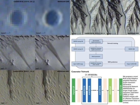
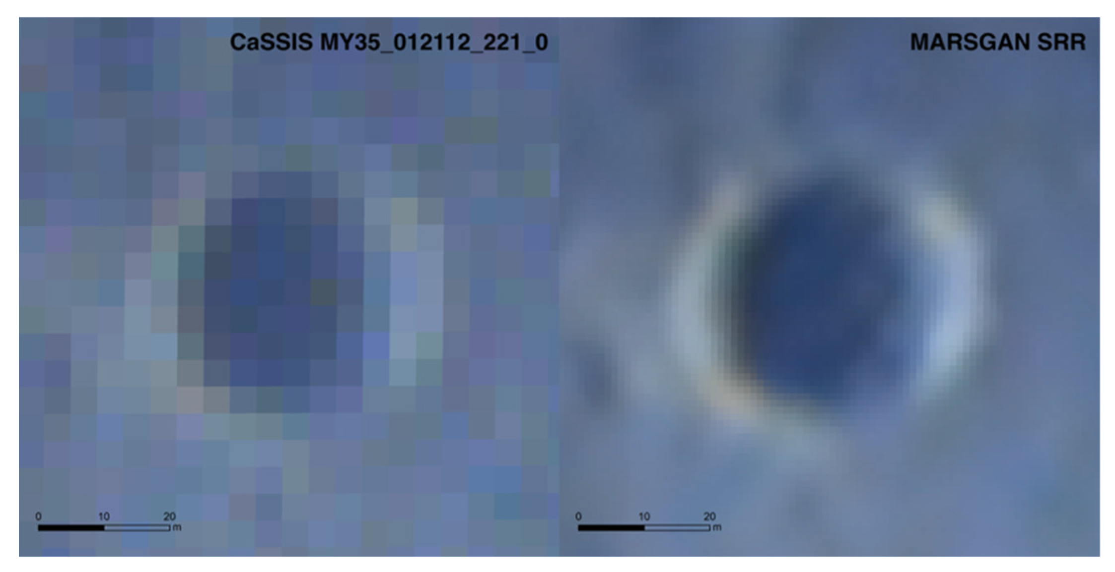
| 4.Gasa Crater | Gullies (-35.731, 129.436) | MY35_012112_221_0 | 2020-08-10 | 15:43 | 255.6° | ESP_065469_1440 | 2020-07-14 | 15:50 | 238.7° |
| 5.Hale Crater | Recurring Slope Lineae (-35.504, 323.454) | MY34_005640_218_1 | 2019-02-27 | 11:09 | 347.9° | ESP_058618_1445 | 2019-01-27 | 14:06 | 331.5° |
| 6.Peneus Patera | Scalloped depressions & Dust Devils (−57.062, 54.544) | MY35_012488_241_0 | 2020-09-10 | 9:36 | 275.1° | ESP_013952_1225 | 2009-07-18 | 14:36 | 305.6° |
| 7.Selevac Crater | Crater & Gullies (-37.386, 228.946) | MY35_012121_222_0 | 2020-08-11 | 15:34 | 256.1° | ESP_065307_1425 | 2020-07-02 | 15:46 | 230.7° |
| 8. South pole | Defrosting Spiders (-74.020, 168.675) | MY35_011777_268_0 | 2020-07-14 | 2:02 | 238.2° | PSP_002081_1055 | 2007-01-05 | 16:15 | 161.8° |
| Area ID | Image | PSNR | MSSIM | BRISQUE % | PIQE % |
|---|---|---|---|---|---|
| A | CaSSIS 4m (upscaled to 1 m) | 26.0443 | 0.4259 | 52.4714 | 89.5445 |
| ESRGAN SRR | 27.4360 | 0.6447 | 45.2599 | 58.2798 | |
| MARSGAN-m1 SRR | 28.3800 | 0.6628 | 44.3843 | 48.1842 | |
| MARSGAN-m2 SRR | 28.8617 | 0.7348 | 40.8888 | 37.9551 | |
| HiRISE 1 m | - | 1.0 | 37.3207 | 17.8052 | |
| B | CaSSIS 4m (upscaled to 1 m) | 25.2536 | 0.5010 | 55.2349 | 89.4813 |
| ESRGAN SRR 1 m | 27.1629 | 0.6266 | 44.8523 | 62.1144 | |
| MARSGAN-m1 SRR 1 m | 27.5165 | 0.7527 | 43.4409 | 58.2852 | |
| MARSGAN-m2 SRR | 27.5788 | 0.7121 | 43.3642 | 57.8908 | |
| HiRISE 1 m | - | 1.0 | 40.0622 | 39.2406 | |
| C | CaSSIS 4m (upscaled to 1 m) | 26.6270 | 0.5890 | 62.2095 | 89.4329 |
| ESRGAN SRR | 27.5628 | 0.6099 | 51.2506 | 53.4608 | |
| MARSGAN-m1 SRR | 28.2237 | 0.7378 | 49.2374 | 52.4337 | |
| MARSGAN-m2 SRR | 28.7730 | 0.7970 | 40.2497 | 37.9989 | |
| HiRISE 1 m | - | 1.0 | 42.8763 | 39.1884 | |
| D | CaSSIS 4m (upscaled to 1 m) | 24.8450 | 0.4129 | 55.6545 | 89.3675 |
| ESRGAN SRR | 26.9355 | 0.5282 | 44.2364 | 69.3333 | |
| MARSGAN-m1 SRR | 27.6077 | 0.5479 | 34.3705 | 54.2366 | |
| MARSGAN-m2 SRR | 28.6258 | 0.6231 | 29.2820 | 45.4305 | |
| HiRISE 1 m | - | 1.0 | 29.5525 | 39.2207 | |
| E | CaSSIS 4m (upscaled to 1 m) | 23.4176 | 0.5025 | 46.6789 | 91.6742 |
| ESRGAN SRR | 24.4753 | 0.7128 | 40.5757 | 89.0071 | |
| MARSGAN-m1 SRR | 24.9328 | 0.7348 | 40.7020 | 75.0569 | |
| MARSGAN-m2 SRR | 25.9999 | 0.7434 | 40.3389 | 54.8428 | |
| HiRISE 1 m | - | 1.0 | 41.9687 | 69.8425 | |
| F | CaSSIS 4m (upscaled to 1 m) | 23.0258 | 0.7153 | 66.6770 | 89.5689 |
| ESRGAN SRR | 25.1195 | 0.8354 | 54.0616 | 55.4445 | |
| MARSGAN-m1 SRR | 24.5218 | 0.8545 | 41.8365 | 47.2499 | |
| MARSGAN-m2 SRR | 25.2674 | 0.8667 | 44.0096 | 48.2412 | |
| HiRISE 1 m | - | 1.0 | 43.4908 | 47.9397 | |
| G | CaSSIS 4m (upscaled to 1 m) | 25.0528 | 0.4539 | 54.5540 | 89.6983 |
| ESRGAN SRR | 26.1769 | 0.6643 | 45.1263 | 69.5151 | |
| MARSGAN-m1 SRR | 26.8709 | 0.7590 | 43.9563 | 57.2191 | |
| MARSGAN-m2 SRR | 27.0346 | 0.7659 | 41.5752 | 58.0473 | |
| HiRISE 1 m | - | 1.0 | 42.4498 | 48.9388 | |
| H | CaSSIS 4m (upscaled to 1 m) | 26.6873 | 0.5973 | 53.3890 | 89.5466 |
| ESRGAN SRR | 27.0394 | 0.7170 | 44.7894 | 69.0773 | |
| MARSGAN-m1 SRR | 27.9313 | 0.7945 | 43.4202 | 63.0145 | |
| MARSGAN-m2 SRR | 28.1564 | 0.8121 | 41.7960 | 58.9527 | |
| HiRISE 1 m | - | 1.0 | 36.9841 | 51.9500 |
| Slanted-Edge ID | CaSSIS Image (Total Number of Pixels for 10–90% Profile Rise) | MARSGAN SRR (Total Number Of Pixels For 10–90% Profile Rise) | ROI Size (Pixels) | Enhancement Factor |
|---|---|---|---|---|
| 1 | 4 | 1.87 | 14 × 12 | 2.14 |
| 2 | 6.36 | 1.86 | 16 × 14 | 3.42 |
| 3 | 6.26 | 2.32 | 19 × 20 | 2.70 |
| 4 | 4.98 | 1.87 | 18 × 21 | 2.66 |
| 5 | 5.80 | 2.31 | 21 × 27 | 2.51 |
| 6 | 6.99 | 2.23 | 26 × 20 | 3.13 |
| 7 | 5.22 | 1.05 | 21 × 21 | 4.97 |
| 8 | 5.81 | 1.98 | 25 × 19 | 2.93 |
| 9 | 5.04 | 1.36 | 20 × 17 | 3.71 |
| 10 | 4.85 | 1.29 | 23 × 22 | 3.76 |
| 11 | 4.19 | 1.59 | 17 × 22 | 2.64 |
| 12 | 5.87 | 2.44 | 22 × 25 | 2.41 |
| 13 | 6.01 | 1.59 | 24 × 19 | 3.78 |
| 14 | 4.19 | 1.84 | 26 × 25 | 2.28 |
| 15 | 6.07 | 2.07 | 16 × 18 | 2.93 |
| 16 | 6.64 | 2.58 | 17 × 16 | 2.57 |
| 17 | 4.45 | 1.56 | 20 × 15 | 2.85 |
| 18 | 6.09 | 1.91 | 23 × 18 | 3.19 |
| 19 | 3.86 | 1.85 | 23 × 17 | 2.09 |
| 20 | 6.21 | 2.41 | 17 × 11 | 2.58 |
| Average | - | - | - | 2.9625 ± 0.7 |
Publisher’s Note: MDPI stays neutral with regard to jurisdictional claims in published maps and institutional affiliations. |
© 2021 by the authors. Licensee MDPI, Basel, Switzerland. This article is an open access article distributed under the terms and conditions of the Creative Commons Attribution (CC BY) license (https://creativecommons.org/licenses/by/4.0/).
Share and Cite
Tao, Y.; Conway, S.J.; Muller, J.-P.; Putri, A.R.D.; Thomas, N.; Cremonese, G. Single Image Super-Resolution Restoration of TGO CaSSIS Colour Images: Demonstration with Perseverance Rover Landing Site and Mars Science Targets. Remote Sens. 2021, 13, 1777. https://doi.org/10.3390/rs13091777
Tao Y, Conway SJ, Muller J-P, Putri ARD, Thomas N, Cremonese G. Single Image Super-Resolution Restoration of TGO CaSSIS Colour Images: Demonstration with Perseverance Rover Landing Site and Mars Science Targets. Remote Sensing. 2021; 13(9):1777. https://doi.org/10.3390/rs13091777
Chicago/Turabian StyleTao, Yu, Susan J. Conway, Jan-Peter Muller, Alfiah R. D. Putri, Nicolas Thomas, and Gabriele Cremonese. 2021. "Single Image Super-Resolution Restoration of TGO CaSSIS Colour Images: Demonstration with Perseverance Rover Landing Site and Mars Science Targets" Remote Sensing 13, no. 9: 1777. https://doi.org/10.3390/rs13091777
APA StyleTao, Y., Conway, S. J., Muller, J.-P., Putri, A. R. D., Thomas, N., & Cremonese, G. (2021). Single Image Super-Resolution Restoration of TGO CaSSIS Colour Images: Demonstration with Perseverance Rover Landing Site and Mars Science Targets. Remote Sensing, 13(9), 1777. https://doi.org/10.3390/rs13091777