
Voxel Grid-Based Fast Registration of Terrestrial Point Cloud

Abstract
1. Introduction
1.1. Background
1.2. Reviews
1.2.1. Keypoints and Feature Points
1.2.2. Four-Point Congruent Sets and Related Methods
1.3. Our Works
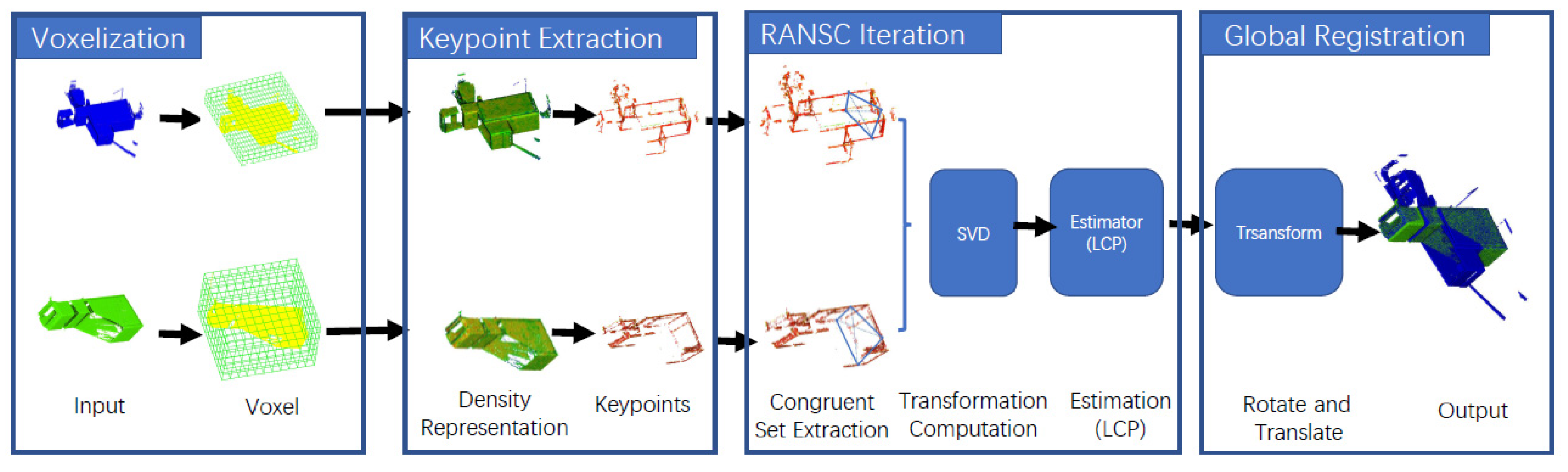
2. Materials and Methods
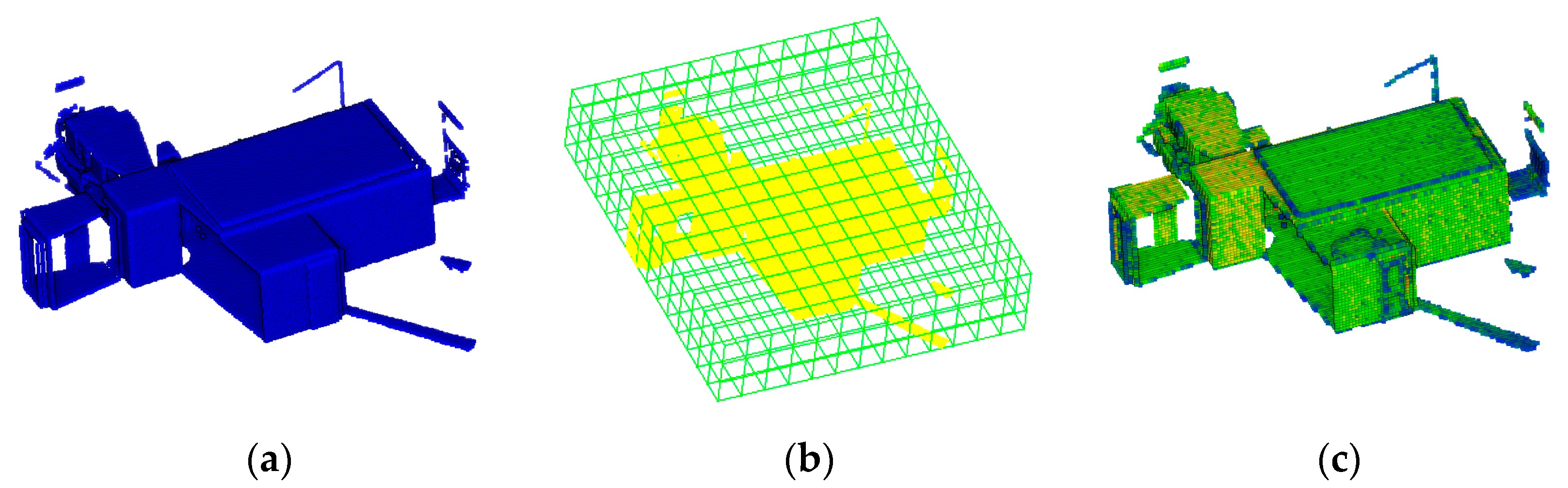
2.1. Voxelization and Indexing Structure Generation
2.2. Keypoint Extraction
2.2.1. Assign Voxel Grid Density Value by Point Distribution
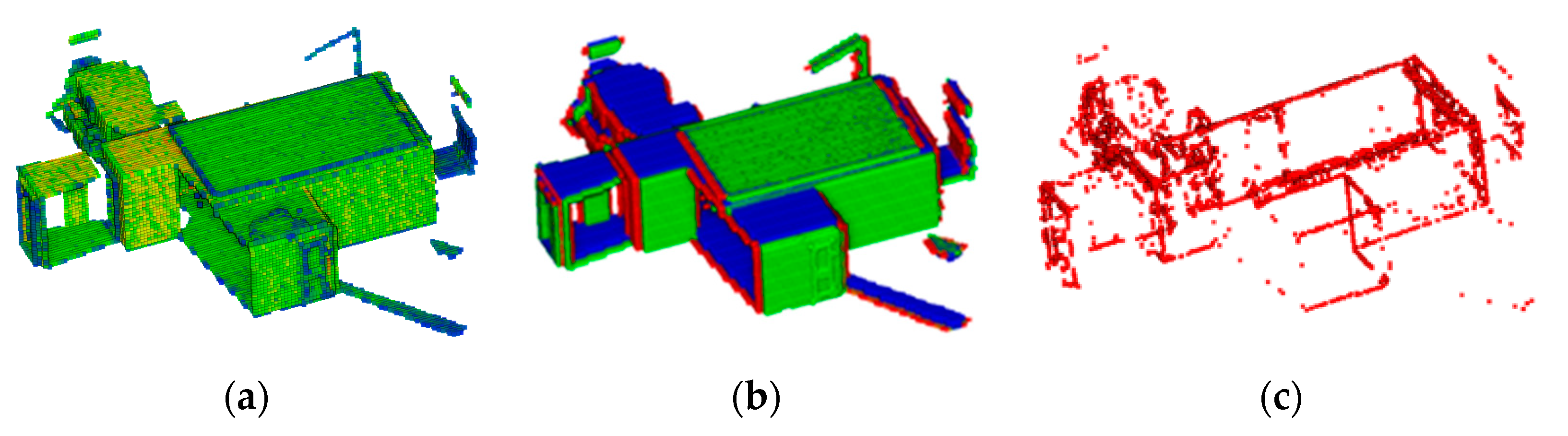
2.2.2. Keypoints Detection by Density Gradient
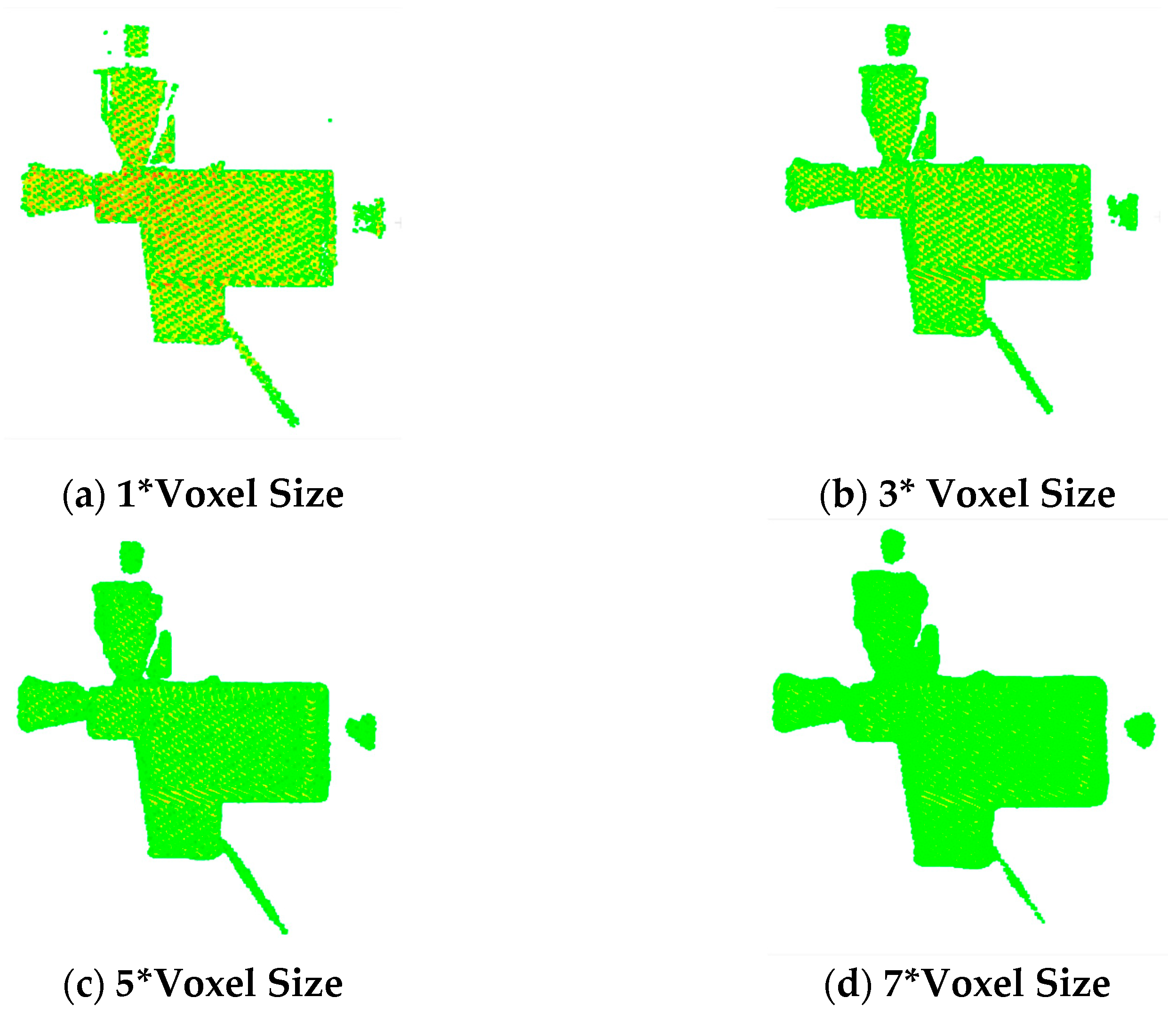
2.2.3. Keypoints Location Optimization
2.3. Voxel-Based 4-Point Congruent Sets
2.3.1. Base for Voxel Grid Filter
2.3.2. Voxel Grid Improved LCP Search
3. Results
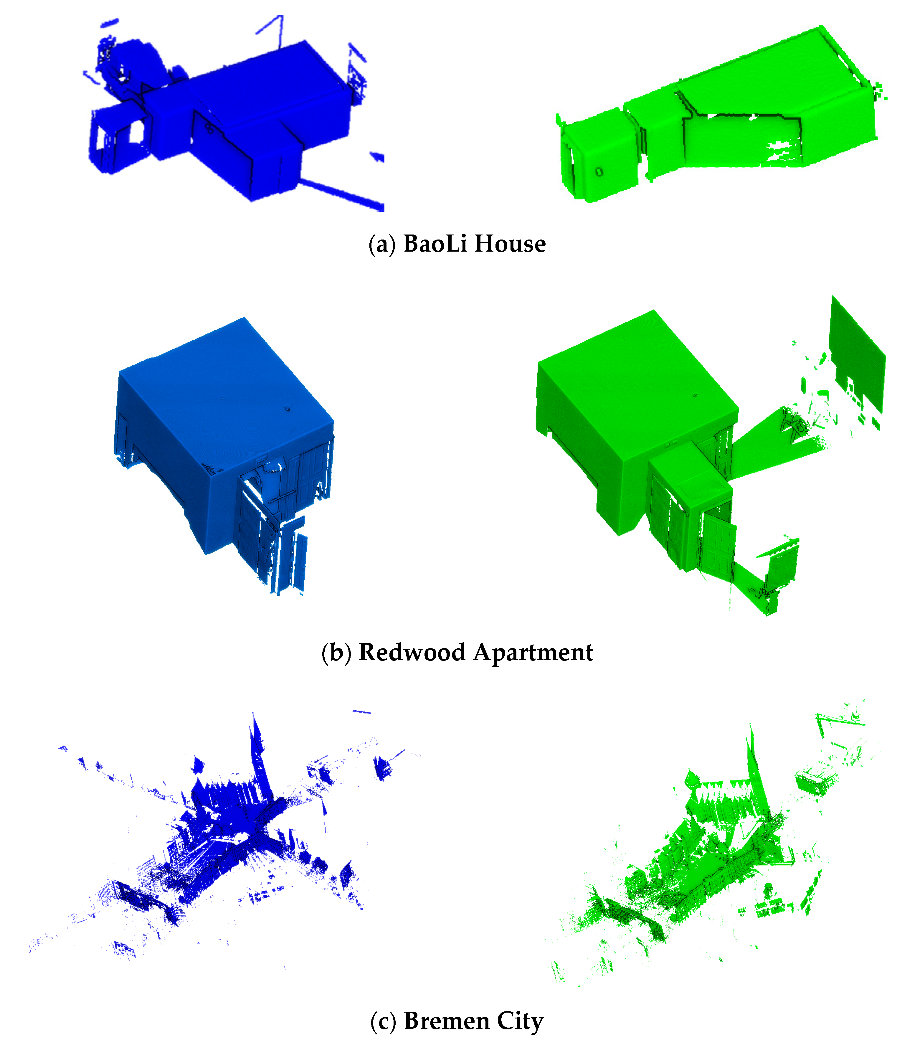
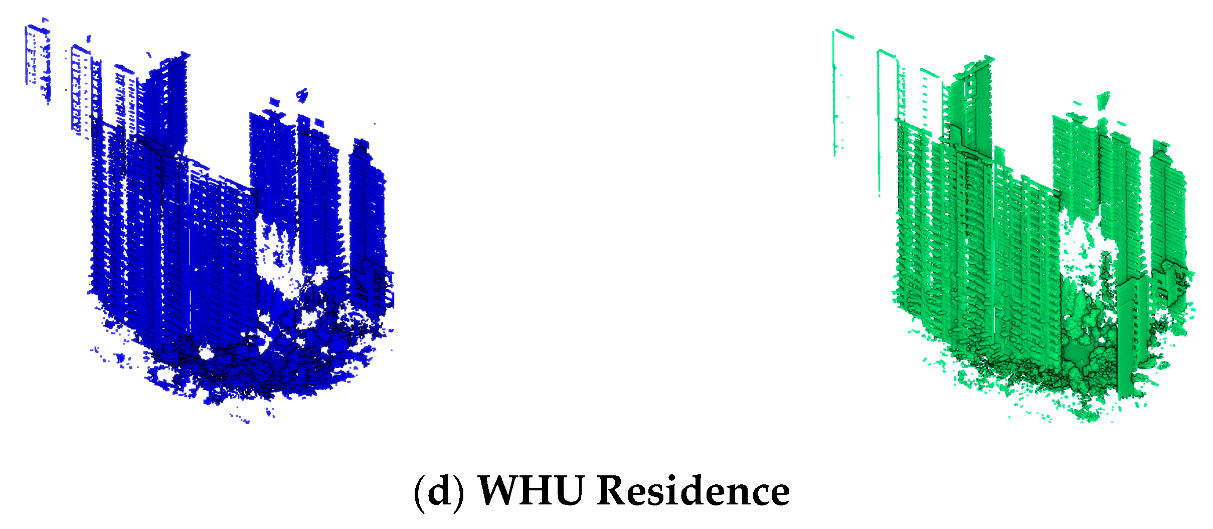
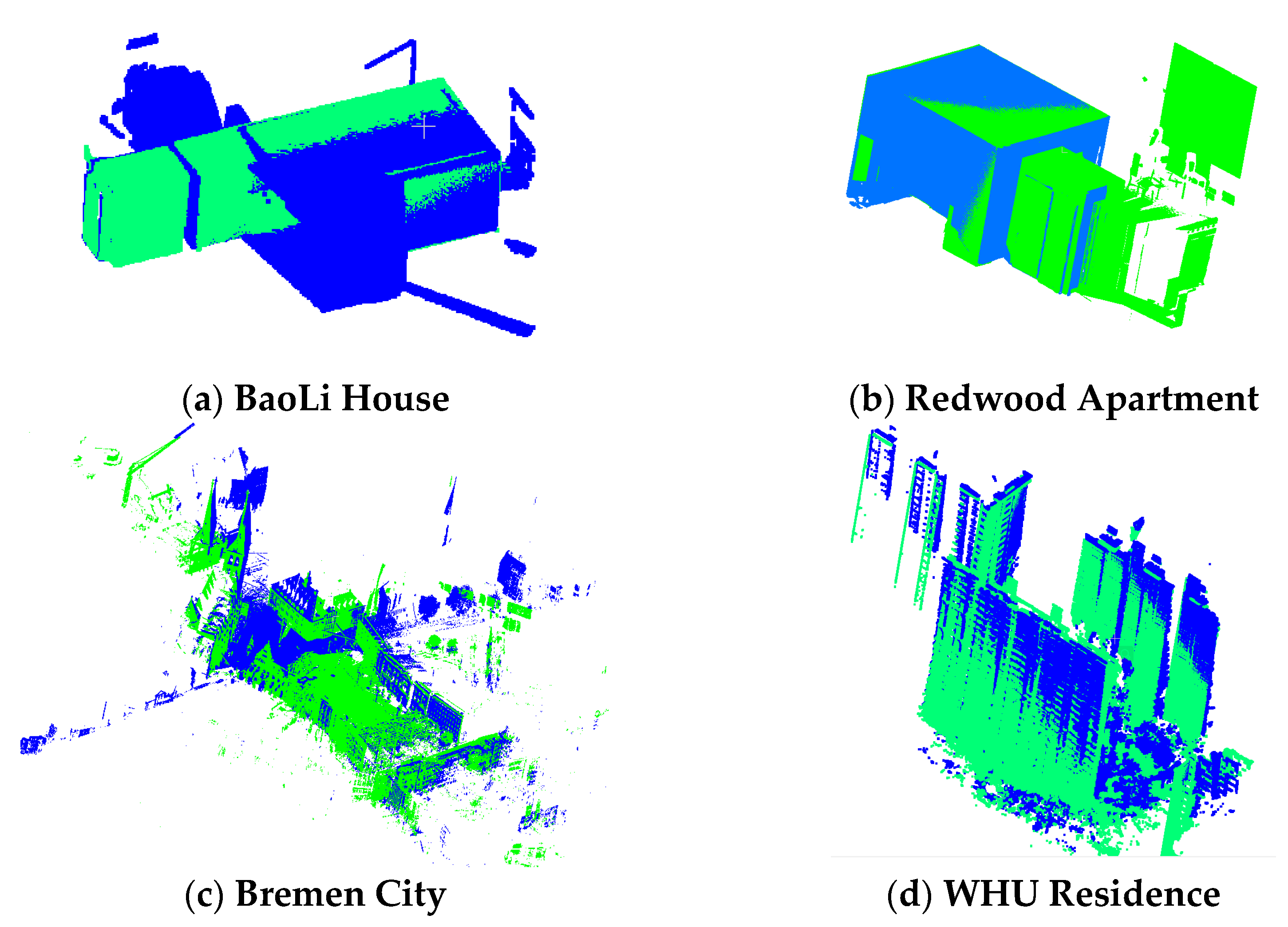
3.1. Experimental Data Sets
3.2. Evaluation Metric
3.2.1. Evaluation Metric of Keypoints Extraction
- (1)
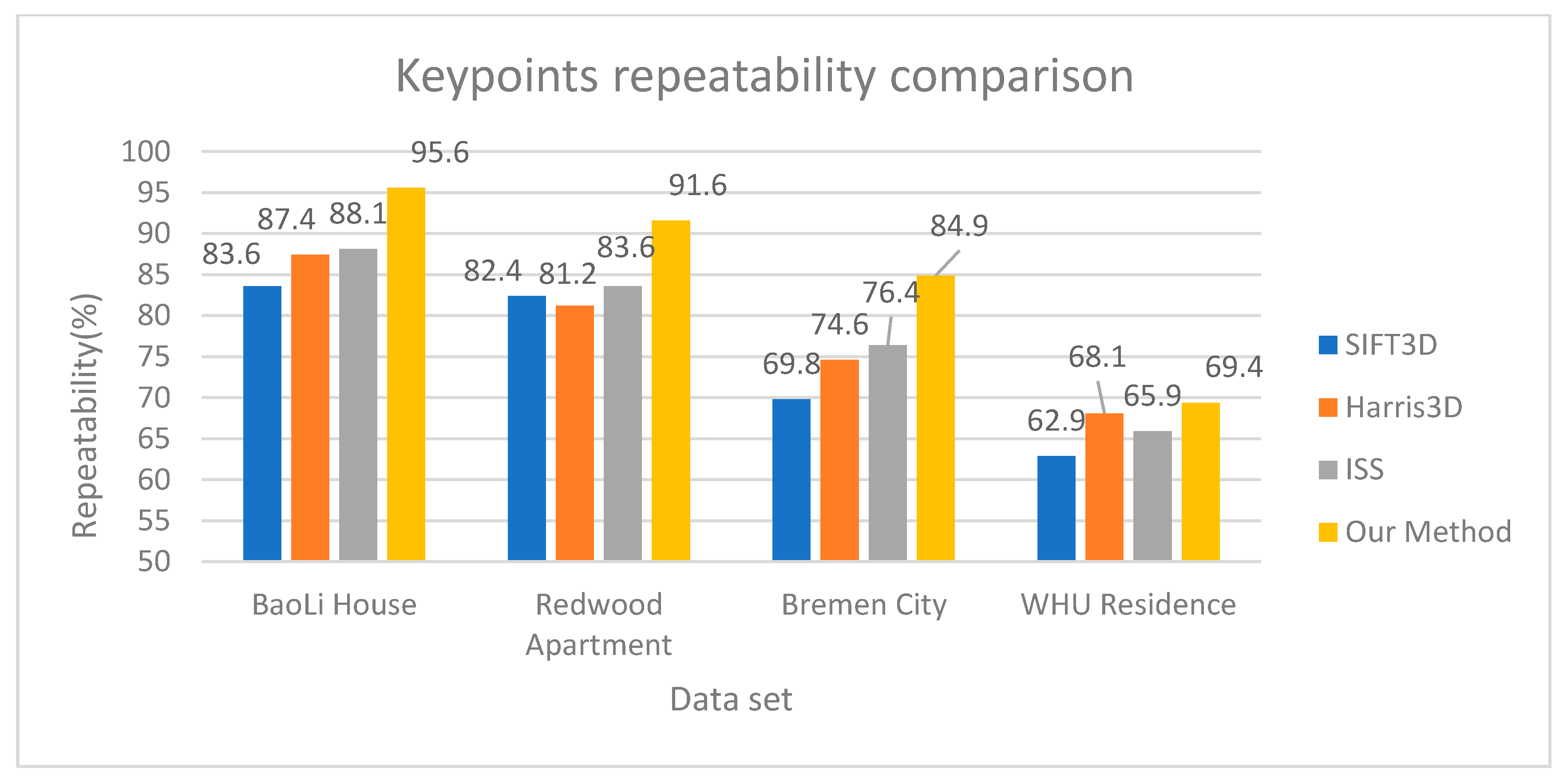
- Repeatability:Given point clouds of the same scene with a different viewpoint, there is a known transformation matrix between the data of the two point clouds. A keypoint detector detects a set of keypoints and from , respectively. A keypoint is repeatable if the distance between and its nearest neighbor is less than the threshold . For the value of in the experiment, we use 0.1 m for indoor data (BaoLi House and Redwood Apartment) and 0.2 m for outdoor data (Bremen City and WHU Residence). The formula for repeatable judgment of keypoint is:The formula for calculating the Repeatability is:where is the number of keypoints in point cloud .
- (2)
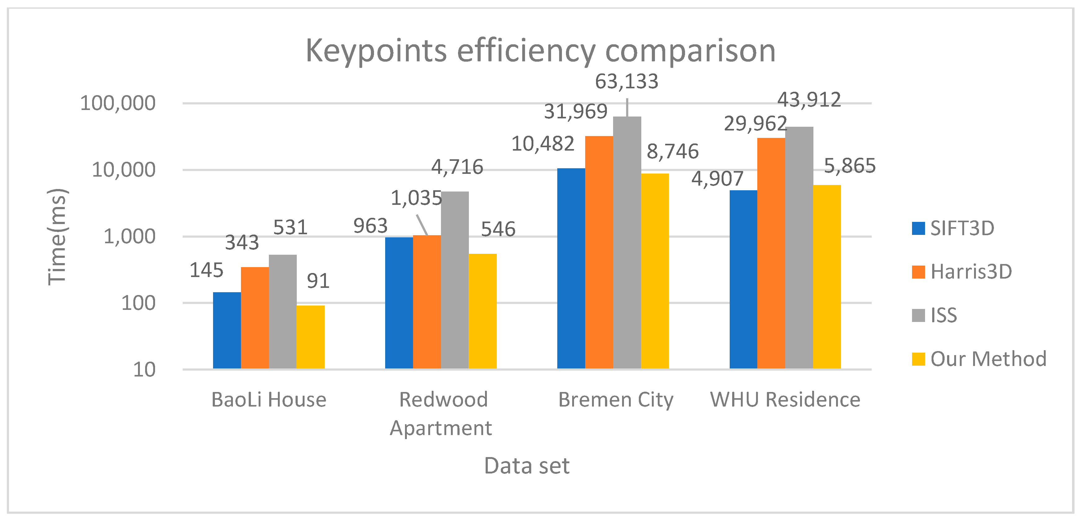
- Efficiency:After defining some parameters, we averaged 50 experimental running times of keypoints detection.
3.2.2. Evaluation Metric of Registration
- (1)
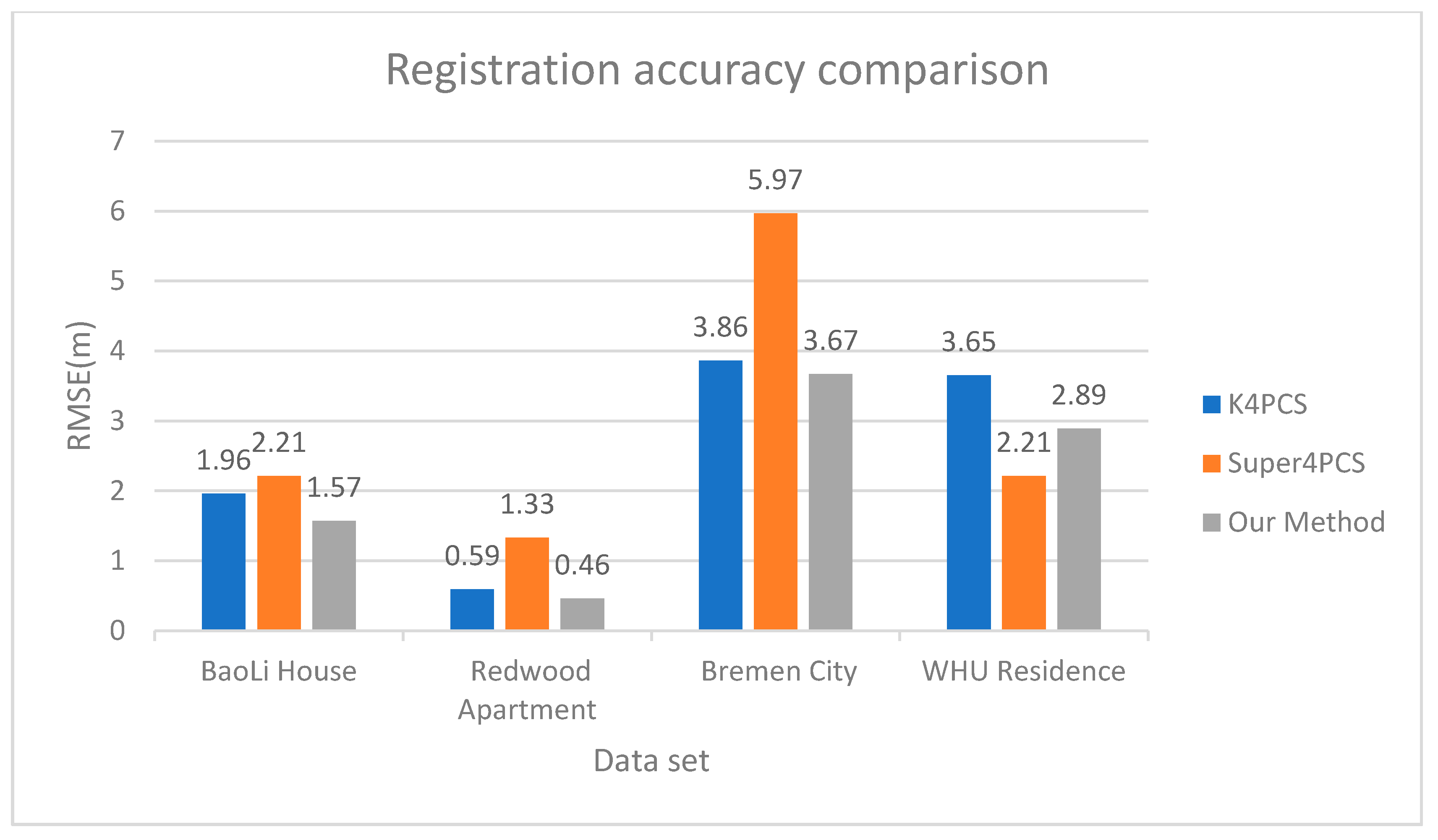
- Registration Accuracy:The root mean square error (RMSE) between the reference registration results of the converted input set was used in evaluating the registration accuracy:where n is the number of points in the point cloud; the i-th point coordinate in the source point cloud S after transformation; and is the i-th point coordinate in the reference registration point cloud.
- (2)
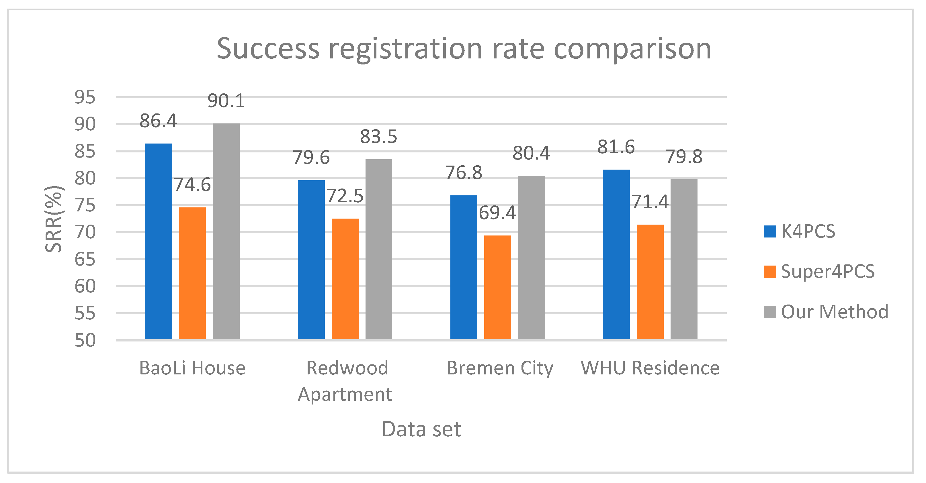
- Success rate:Based on the root mean error, the registration success rate (RS) can be directly calculated using the formula:The RMSE threshold can be set according to the application requirements. The formula for calculating the successful registration rate (SRR) is:where is the number of successful registrations, and N is the number of experiments. Since our method involves the RANSAC process, SRR is evaluated in a series of 50 trials.
- (3)
- Computational Efficiency:The calculation efficiency is evaluated using the average total running time Tt of the entire process. Take the average of 500 experimental data for the overall coarse registration.
3.3. Keypoints Extraction
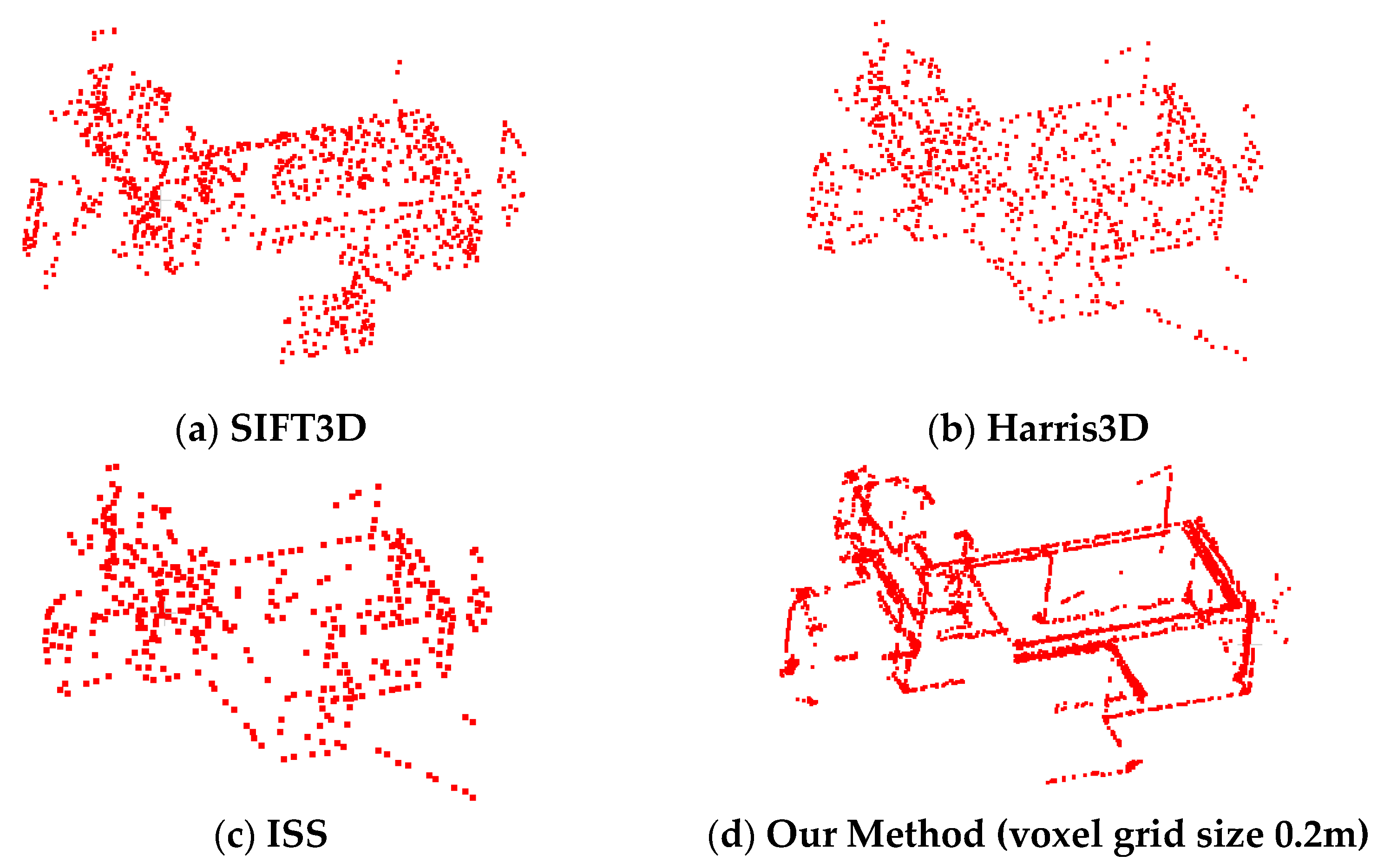
3.4. Keypoints Comparison
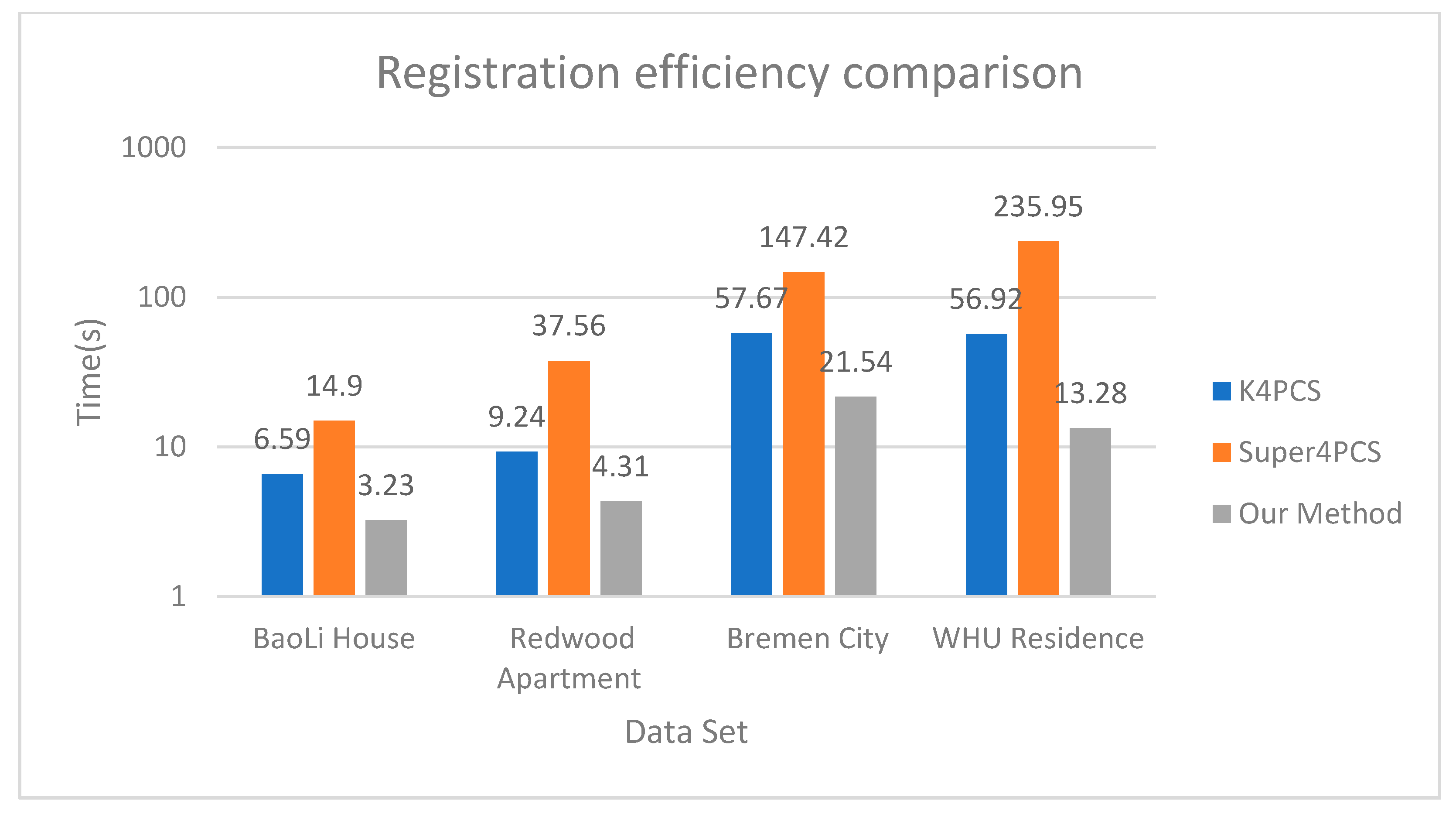
3.5. Registraion Time Performance
3.6. Registration Accuracy
3.7. Registration Comparison and Analysis
4. Discussion
5. Conclusions
Author Contributions
Funding
Informed Consent Statement
Data Availability Statement
Acknowledgments
Conflicts of Interest
References
- Dos Santos, D.R.; Basso, M.A.; Khoshelham, K.; de Oliveira, E.; Pavan, N.L.; Vosselman, G. Mapping indoor spaces by adaptive coarse-to-fine registration of RGB-D data. IEEE Geosci. Remote Sens. Lett. 2016, 13, 262–266. [Google Scholar] [CrossRef]
- Ma, W.; Wu, Y.; Zheng, Y.; Wen, Z.; Liu, L. Remote sensing image registration based on multifeature and region division. IEEE Geosci. Remote Sens. Lett. 2017, 14, 1680–1684. [Google Scholar] [CrossRef]
- Wang, Y.; Xiao, J.; Liu, L.; Wang, Y. Efficient rock mass point cloud registration based on local invariants. Remote Sens. 2021, 13, 1540. [Google Scholar]
- Besl, P.J.; McKay, N.D. A method for registration of 3-D shapes. IEEE Trans. Pattern Anal. Mach. Intell. 1992, 14, 239–256. [Google Scholar] [CrossRef]
- Gelfand, N.; Ikemoto, L.; Rusinkiewicz, S.; Levoy, M. Geometrically stable sampling for the ICP algorithm. In Proceedings of the 4th International Conference on 3-D Digital Imaging and Modeling, Banff, AB, Canada, 6–10 October 2003; pp. 260–267. [Google Scholar]
- Yang, J.; Li, H.; Jia, Y. Go-icp: Solving 3d registration efficiently and globally optimally. In Proceedings of the IEEE International Conference on Computer Vision, Sydney, Australia, 1–8 December 2013; pp. 1457–1464. [Google Scholar]
- Rusinkiewicz, S. A symmetric objective function for ICP. ACM Trans. Graph. 2019, 38, 1–7. [Google Scholar] [CrossRef]
- Cai, Z.; Chin, T.J.; Bustos, A.P.; Schindler, K. Practical optimal registration of terrestrial LiDAR scan pairs. ISPRS J. Photogramm. Remote Sens. 2019, 147, 118–131. [Google Scholar] [CrossRef]
- Harris, C.; Stephens, M. A combined corner and edge detection. In Proceedings of the 4th Alvey Vision Conference, Manchester, UK, 31 August–2 September 1988; pp. 147–151. [Google Scholar]
- Ambühl, C.; Chakraborty, S.; Gärtner, B. Computing largest common point sets under approximate congruence. In Proceedings of the 8th Annual European Symposium, Saarbrücken, Germany, 5–8 September 2000; Springer: Berlin/Heidelberg, Germany, 2000; pp. 52–64. [Google Scholar]
- Lowe, D.G. Object recognition from local scale-invariant features. In Proceedings of the 7th IEEE International Conference on Computer Vision, Kerkyra, Greece, 20–27 September 1999; pp. 1150–1157. [Google Scholar]
- Lowe, D.G. Distinctive image features from scale-invariant keypoints. Int. J. Comput. Vis. 2004, 60, 91–110. [Google Scholar] [CrossRef]
- Lindeberg, T. Scale Invariant Feature Transform. 2012. Available online: http://www.scholarpedia.org/article/Scale_Invariant_Feature_Transform (accessed on 11 May 2021).
- Sipiran, I.; Bustos, B. Harris 3D: A robust extension of the Harris operator for interest point detection on 3D meshes. Vis. Comput. 2011, 27, 963–976. [Google Scholar] [CrossRef]
- Zhong, Y. Intrinsic shape signatures: A shape descriptor for 3d object recognition. In Proceedings of the 2009 IEEE 12th International Conference on Computer Vision Workshops, Kyoto, Japan, 26 September–4 October 2009; pp. 689–696. [Google Scholar]
- Zai, D.; Li, J.; Guo, Y.; Cheng, M.; Huang, P.; Cao, X.; Wang, C. Pairwise registration of TLS point clouds using covariance descriptors and a non-cooperative game. ISPRS J. Photogramm. Remote Sens. 2017, 134, 15–29. [Google Scholar] [CrossRef]
- Handte, M.; Iqbal, U.; Apolinarski, W.; Wagner, S.; Marrón, P.J. The narf architecture for generic personal context recognition. In Proceedings of the 2010 IEEE International Conference on Sensor Networks, Ubiquitous, and Trustworthy Computing, Newport Beach, CA, USA, 7–9 June 2010; pp. 123–130. [Google Scholar]
- Rusu, R.B.; Blodow, N.; Marton, Z.C.; Beetz, M. Aligning point cloud views using persistent feature histograms. In Proceedings of the 2008 IEEE/RSJ International Conference on Intelligent Robots and Systems, Nice, France, 22–26 September 2008; pp. 3384–3391. [Google Scholar]
- Rusu, R.B.; Blodow, N.; Beetz, M. Fast point feature histograms (FPFH) for 3D registration. In Proceedings of the 2009 IEEE International Conference on Robotics and Automation, Kobe, Japan, 12–17 May 2009; pp. 3212–3217. [Google Scholar]
- Frome, A.; Huber, D.; Kolluri, R.; Bülow, T.; Malik, J. Recognizing objects in range data using regional point descriptors. In Proceedings of the 8th European Conference on Computer Vision, Prague, Czech Republic, 11–14 May 2004; Springer: Berlin/Heidelberg, Germany, 2004; pp. 224–237. [Google Scholar]
- Dong, Z.; Yang, B.; Liang, F.; Huang, R.; Scherer, S. Hierarchical registration of unordered TLS point clouds based on binary shape context descriptor. ISPRS J. Photogramm. Remote Sens. 2018, 144, 61–79. [Google Scholar] [CrossRef]
- Qi, C.R.; Su, H.; Mo, K.; Guibas, L.J. Pointnet: Deep learning on point sets for 3d classification and segmentation. In Proceedings of the IEEE Conference on Computer Vision and Pattern Recognition, Honolulu, HI, USA, 21–26 July 2017; pp. 652–660. [Google Scholar]
- Qi, C.R.; Yi, L.; Su, H.; Guibas, L.J. PointNet++ deep hierarchical feature learning on point sets in a metric space. In Proceedings of the 31st International Conference on Neural Information Processing Systems, Long Beach, CA, USA, 4–9 December 2017; pp. 5105–5114. [Google Scholar]
- Wu, W.; Zhang, Y.; Wang, D.; Lei, Y. SK-Net: Deep learning on point cloud via end-to-end discovery of spatial keypoints. In Proceedings of the AAAI Conference on Artificial Intelligence, New York, NY, USA, 7–12 February 2020; pp. 6422–6429. [Google Scholar]
- Yew, Z.J.; Lee, G.H. 3dfeat-net: Weakly supervised local 3d features for point cloud registration. In Proceedings of the European Conference on Computer Vision (ECCV), Munich, Germany, 8–14 September 2018; pp. 607–623. [Google Scholar]
- Li, J.; Lee, G.H. Usip: Unsupervised stable interest point detection from 3d point clouds. In Proceedings of the IEEE/CVF International Conference on Computer Vision, Seoul, Korea, 27–28 October 2019; pp. 361–370. [Google Scholar]
- Fischler, M.A.; Bolles, R.C. Random sample consensus: A paradigm for model fitting with applications to image analysis and automated cartography. In Readings in Computer Vision; Elsevier: Amsterdam, The Netherlands, 1987; pp. 726–740. [Google Scholar]
- Aiger, D.; Mitra, N.J.; Cohen-Or, D. 4-points congruent sets for robust pairwise surface registration. ACM Trans. Graph. 2008, 1–10. [Google Scholar] [CrossRef]
- Mellado, N.; Aiger, D.; Mitra, N.J. Super 4pcs fast global pointcloud registration via smart indexing. Comput. Graph. Forum 2014, 205–215. [Google Scholar] [CrossRef]
- Mohamad, M.; Rappaport, D.; Greenspan, M. Generalized 4-points congruent sets for 3d registration. In Proceedings of the 2014 2nd International Conference on 3D Vision, Tokyo, Japan, 8–11 December 2014; pp. 83–90. [Google Scholar]
- Mohamad, M.; Ahmed, M.T.; Rappaport, D.; Greenspan, M. Super generalized 4pcs for 3d registration. In Proceedings of the 2015 International Conference on 3D Vision, Lyon, France, 19–22 October 2015; pp. 598–606. [Google Scholar]
- Huang, J.; Kwok, T.-H.; Zhou, C. V4PCS: Volumetric 4PCS algorithm for global registration. J. Mech. Des. 2017, 139, 111403. [Google Scholar] [CrossRef]
- Zhang, R.; Li, H.; Liu, L.; Wu, M. A G-super4PCS registration method for photogrammetric and TLS data in geology. ISPRS Int. J. GeoInf. 2017, 6, 129. [Google Scholar] [CrossRef]
- Theiler, P.W.; Wegner, J.D.; Schindler, K.; Sciences, S.I. Markerless point cloud registration with keypoint-based 4-points congruent sets. ISPRS Ann. Photogramm. Remote Sens. Spat. Inf. Sci. 2013, 1, 283–288. [Google Scholar] [CrossRef]
- Theiler, P.W.; Wegner, J.D.; Schindler, K. Keypoint-based 4-points congruent sets–automated marker-less registration of laser scans. ISPRS J. Photogramm. Remote Sens. 2014, 96, 149–163. [Google Scholar] [CrossRef]
- Theiler, P.W.; Wegner, J.D.; Schindler, K. Fast registration of laser scans with 4-points congruent sets-what works and what doesn’t. ISPRS Ann. Photogramm. Remote Sens. Spat. Inf. Sci. 2014, 2, 149–156. [Google Scholar] [CrossRef]
- Ge, X.; Sensing, R. Automatic markerless registration of point clouds with semantic-keypoint-based 4-points congruent sets. ISPRS J. Photogramm. Remote Sens. 2017, 130, 344–357. [Google Scholar] [CrossRef]
- Xu, Z.; Xu, E.; Zhang, Z.; Wu, L. Multiscale sparse features embedded 4-points congruent sets for global registration of TLS point clouds. IEEE Geosci. Remote Sens. Lett. 2018, 16, 286–290. [Google Scholar] [CrossRef]
- Sun, J.; Zhang, R.; Du, S.; Zhang, L.; Liu, Y. Global adaptive 4-points congruent sets registration for 3D indoor scenes with robust estimation. IEEE Access 2020, 8, 7539–7548. [Google Scholar] [CrossRef]
- Yang, B.; Dong, Z.; Liang, F.; Liu, Y. Automatic registration of large-scale urban scene point clouds based on semantic feature points. ISPRS J. Photogramm. Remote Sens. 2016, 113, 43–58. [Google Scholar] [CrossRef]
- Xu, Y.; Boerner, R.; Yao, W.; Hoegner, L.; Stilla, U. Pairwise coarse registration of point clouds in urban scenes using voxel-based 4-planes congruent sets. ISPRS J. Photogramm. Remote Sens. 2019, 151, 106–123. [Google Scholar] [CrossRef]
- Park, J.; Zhou, Q.Y.; Koltun, V. Colored point cloud registration revisited. In Proceedings of the International Conference on Computer Vision, Venice, Italy, 23–29 October 2017. [Google Scholar]
- Borrmann, D.; Elseberg, J.; Lingemann, K.; Nüchter, A.; Hertzberg, J.J.R. Globally consistent 3D mapping with scan matching. Robot. Auton. Syst. 2008, 56, 130–142. [Google Scholar] [CrossRef]
- Dong, Z.; Liang, F.; Yang, B.; Xu, Y.; Zang, Y.; Li, J.; Wang, Y.; Dai, W.; Fan, H.; Hyyppä, J.; et al. Registration of large-scale terrestrial laser scanner point clouds: A review and benchmark. ISPRS J. Photogramm. Remote Sens. 2020, 163, 327–342. [Google Scholar] [CrossRef]


| Parameters | BaoLi House | Redwood Apartment | Bremen City | WHU Residence | |||||
|---|---|---|---|---|---|---|---|---|---|
| Source | Target | Source | Target | Source | Target | Source | Target | ||
| Dimension of bounding box(m) | X | 12.79 | 10.51 | 3.96 | 7.51 | 526.63 | 336.67 | 239.77 | 271.61 |
| Y | 14.30 | 6.78 | 6.01 | 8.08 | 651.84 | 684.12 | 117.32 | 150.59 | |
| Z | 2.77 | 9.47 | 2.86 | 2.75 | 120.51 | 96.05 | 92.99 | 96.77 | |
| Number of Points (thousand) | 9250 | 10749 | 1492 | 2174 | 7484 | 6885 | 5820 | 6145 | |
| RMSE (m) | 0.95 | 0.09 | 3.59 | 1.64 | |||||
| Data Set | Voxel | Source Scan | Target Scan | ||||
|---|---|---|---|---|---|---|---|
| Size (m) | Key Points | Repeat-Ability | Time (ms) | Key Points | Repeat-Ability | Time (ms) | |
| BaoLi House | 0.1 | 5487 | 96.1 | 36 | 5334 | 97.2 | 24 |
| 0.2 | 2248 | 95.6 | 91 | 2443 | 95.9 | 54 | |
| 0.5 | 515 | 92.3 | 307 | 780 | 92.8 | 185 | |
| Redwood Apartment | 0.1 | 1864 | 92.7 | 267 | 2643 | 89.4 | 374 |
| 0.2 | 897 | 91.6 | 546 | 1022 | 87.5 | 851 | |
| 0.5 | 184 | 87.6 | 1344 | 342 | 84.3 | 1546 | |
| Bremen City | 0.1 | 152,416 | 91.2 | 1896 | 186,421 | 90.6 | 2173 |
| 0.2 | 64,185 | 88.6 | 3859 | 81,638 | 87.4 | 4681 | |
| 0.5 | 21,067 | 84.9 | 8746 | 24,025 | 84.1 | 9857 | |
| WHT Residence | 0.1 | 196,492 | 77.6 | 1154 | 172,649 | 76.5 | 1274 |
| 0.2 | 72,991 | 74.2 | 1978 | 63,594 | 73.6 | 2027 | |
| 0.5 | 40,050 | 69.4 | 5865 | 10,370 | 70.1 | 5304 | |
| Data Set | Voxel Size(m) | Candidate Set Number | Keypoints Detection Time (s) | Time (s) |
|---|---|---|---|---|
| BaoLi House | 0.1 | 2221 | 0.06 | 3.28 |
| 0.2 | 1872 | 0.14 | 3.23 | |
| 0.5 | 118 | 0.49 | 1.49 | |
| Redwood Apartment | 0.1 | 5016 | 0.64 | 6.58 |
| 0.2 | 2036 | 1.39 | 4.31 | |
| 0.5 | 849 | 2.89 | 4.65 | |
| Bremen City | 0.1 | 24,311 | 4.07 | 41.78 |
| 0.2 | 8604 | 8.54 | 22.46 | |
| 0.5 | 2673 | 18.6 | 21.54 | |
| WHU Residence | 0.1 | 8643 | 2.43 | 15.46 |
| 0.2 | 4269 | 4.01 | 7.74 | |
| 0.5 | 1563 | 11.16 | 13.28 |
| Data Set | Voxel Size (m) | Pairs Number | Candidate Set Number | RMSE (M) | SRR (%) | Time (s) |
|---|---|---|---|---|---|---|
| BaoLi House | 0.1 | 1839 | 2221 | 2.42 | 95.0 | 3.28 |
| 0.2 | 1680 | 1872 | 1.57 | 90.1 | 3.23 | |
| 0.5 | 1257 | 118 | 1.26 | 84.6 | 1.49 | |
| Redwood Apartment | 0.1 | 2844 | 5016 | 0.39 | 89.2 | 6.58 |
| 0.2 | 1484 | 2036 | 0.46 | 83.5 | 4.31 | |
| 0.5 | 536 | 849 | 0.84 | 77.4 | 4.65 | |
| Bremen City | 0.1 | 8469 | 24,311 | 2.86 | 86.7 | 41.78 |
| 0.2 | 3024 | 8604 | 2.28 | 83.4 | 22.46 | |
| 0.5 | 1541 | 2673 | 3.67 | 80.4 | 21.54 | |
| WHU Residence | 0.1 | 3416 | 8643 | 2.54 | 85.5 | 15.46 |
| 0.2 | 2218 | 4269 | 3.38 | 82.4 | 7.74 | |
| 0.5 | 1280 | 1563 | 2.89 | 79.8 | 13.28 |
| Data Set | Method | Pairs Number | Candidate Set Number | RMSE (m) | SRR (%) | Time (s) | Efficiency Improve (%) |
|---|---|---|---|---|---|---|---|
| BaoLi House | K4PCS | 7114 | 2762 | 1.96 | 86.4 | 6.59 | 50 |
| Super4PCS | 8874 | 54,721 | 2.21 | 74.6 | 14.9 | 78 | |
| Our Method | 1680 | 1872 | 1.57 | 90.1 | 3.23 | ||
| Redwood Apartment | K4PCS | 1493 | 3749 | 0.59 | 79.6 | 9.24 | 53 |
| Super4PCS | 3747 | 11,389 | 1.33 | 72.5 | 37.56 | 88 | |
| Our Method | 1484 | 2036 | 0.46 | 83.5 | 4.31 | ||
| Bremen City | K4PCS | 2186 | 5462 | 3.86 | 76.8 | 57.67 | 62 |
| Super4PCS | 4419 | 35,449 | 5.97 | 69.4 | 147.42 | 85 | |
| Our Method | 1541 | 2673 | 3.67 | 80.4 | 21.54 | ||
| WHU Residence | K4PCS | 5734 | 6190 | 3.65 | 81.6 | 56.92 | 76 |
| Super4PCS | 12,588 | 33,403 | 2.21 | 71.4 | 235.95 | 94 | |
| Our Method | 1280 | 1563 | 2.89 | 79.8 | 13.28 |
| Method | Number of Points | |||
|---|---|---|---|---|
| 10,000 Random Points Data | 100,000 Random Points Data | 1,000,000 Random Points Data | ||
| 1,000,000 query time (ms) | KD-Tree | 83 | 106 | 131 |
| Our Method | 60 | 59 | 63 | |
| 100,000,000 query time (ms) | KD-Tree | 8264 | 9838 | 12,406 |
| Our Method | 5881 | 5948 | 6057 | |
Publisher’s Note: MDPI stays neutral with regard to jurisdictional claims in published maps and institutional affiliations. |
© 2021 by the authors. Licensee MDPI, Basel, Switzerland. This article is an open access article distributed under the terms and conditions of the Creative Commons Attribution (CC BY) license (https://creativecommons.org/licenses/by/4.0/).
Share and Cite
Xiong, B.; Jiang, W.; Li, D.; Qi, M. Voxel Grid-Based Fast Registration of Terrestrial Point Cloud. Remote Sens. 2021, 13, 1905. https://doi.org/10.3390/rs13101905
Xiong B, Jiang W, Li D, Qi M. Voxel Grid-Based Fast Registration of Terrestrial Point Cloud. Remote Sensing. 2021; 13(10):1905. https://doi.org/10.3390/rs13101905
Chicago/Turabian StyleXiong, Biao, Weize Jiang, Dengke Li, and Man Qi. 2021. "Voxel Grid-Based Fast Registration of Terrestrial Point Cloud" Remote Sensing 13, no. 10: 1905. https://doi.org/10.3390/rs13101905
APA StyleXiong, B., Jiang, W., Li, D., & Qi, M. (2021). Voxel Grid-Based Fast Registration of Terrestrial Point Cloud. Remote Sensing, 13(10), 1905. https://doi.org/10.3390/rs13101905