Article

A Scalable Machine Learning Pipeline for Paddy Rice Classification Using Multi-Temporal Sentinel Data

by
Vasileios Sitokonstantinou
1,2,*,
Alkiviadis Koukos
1,
Thanassis Drivas
1,
Charalampos Kontoes
1,
Ioannis Papoutsis
1 and
Vassilia Karathanassi
2
1
Institute for Space Applications and Remote Sensing, National Observatory of Athens, I. Metaxa and Vas. Pavlou St, Penteli, 15236 Athens, Greece
2
Laboratory of Remote Sensing, National Technical University of Athens, 9 Heroon Polytechniou Str., Zographos, 15790 Athens, Greece
*
Author to whom correspondence should be addressed.
Remote Sens. 2021, 13(9), 1769; https://doi.org/10.3390/rs13091769
Submission received: 31 March 2021 / Revised: 23 April 2021 / Accepted: 28 April 2021 / Published: 1 May 2021
(This article belongs to the Section AI Remote Sensing)

Abstract

:
The demand for rice production in Asia is expected to increase by 70% in the next 30 years, which makes evident the need for a balanced productivity and effective food security management at a national and continental level. Consequently, the timely and accurate mapping of paddy rice extent and its productivity assessment is of utmost significance. In turn, this requires continuous area monitoring and large scale mapping, at the parcel level, through the processing of big satellite data of high spatial resolution. This work designs and implements a paddy rice mapping pipeline in South Korea that is based on a time-series of Sentinel-1 and Sentinel-2 data for the year of 2018. There are two challenges that we address; the first one is the ability of our model to manage big satellite data and scale for a nationwide application. The second one is the algorithm’s capacity to cope with scarce labeled data to train supervised machine learning algorithms. Specifically, we implement an approach that combines unsupervised and supervised learning. First, we generate pseudo-labels for rice classification from a single site (Seosan-Dangjin) by using a dynamic k-means clustering approach. The pseudo-labels are then used to train a Random Forest (RF) classifier that is fine-tuned to generalize in two other sites (Haenam and Cheorwon). The optimized model was then tested against 40 labeled plots, evenly distributed across the country. The paddy rice mapping pipeline is scalable as it has been deployed in a High Performance Data Analytics (HPDA) environment using distributed implementations for both k-means and RF classifiers. When tested across the country, our model provided an overall accuracy of 96.69% and a kappa coefficient 0.87. Even more, the accurate paddy rice area mapping was returned early in the year (late July), which is key for timely decision-making. Finally, the performance of the generalized paddy rice classification model, when applied in the sites of Haenam and Cheorwon, was compared to the performance of two equivalent models that were trained with locally sampled labels. The results were comparable and highlighted the success of the model’s generalization and its applicability to other regions.

Graphical Abstract

1. Introduction

Over the last decades, the continuous increase in global population and need for nutrition, in combination with the impact of climate change on food production, is expected to affect the food sector significantly [1]. The agricultural productivity needs to be strengthened in order to accommodate the needs of the growing population, while preserving environmentally-friendly and sustainable agricultural practices. In this context, there is a need for the timely, large-scale and accurate monitoring of agricultural production and the provision of the necessary knowledge for evidence-based decision making on food security matters [1,2].
Rice is a widely planted crop in the world and the most important food staple in Asia. Merely fifteen Asian countries, including South Korea that is the study area of this work, account for 90% of the global rice production and the demand is expected to increase by 70% in the next 30 years [3]. These figures indicate that there is pressing need for timely and accurate knowledge for rice’s spatial distribution and its expected yield at national and continental scales [4].
According to the Korean Statistical Information Service (KOSIS), South Korea cultivates approximately 730 thousand hectares and produces more than 3.5 million tonnes of rice annually, which amounts to 0.5% of the global rice production. Furthermore, the global food security index by the Economist Intelligence Unit ranks South Korea’s performance at the top 30 (29/113), with a score 72.1. However, there is systematic overproduction of rice that results in large storage costs and shortage in other major grains. This is due to the governmental direct payment scheme that focuses on rice and gives limited incentives for the cultivation of other crops [5]. Even more, South Korea scores a negative 85%, referring to the percentage difference from the mean global score, in the crop storage facility indicator of the global food security index. This indicator is based on the assessment on the governmental investments to improve crop storage.
To address the required large-scale monitoring of agricultural production, Earth Observation (EO) data are widely used and constitute a unique basis for deriving the necessary information. For the purposes of food security monitoring, the Food and Agriculture Organization of the United Nations (FAO), the European Union (EU), but also global and regional initiatives such as the Group on Earth Observations Global Agricultural Monitoring (GEOGLAM) and Asian Rice Crop Estimation and Monitoring (Asia-RiCE), have invested greatly in the exploitation of EO to monitor the extent, health, growth and productivity of the agricultural land over very large areas [6,7,8,9].
The monitoring and mapping of paddy rice extent in South Korea and the estimation of its productivity is currently performed by the Korea Rural Economic Institute (KREI). The current approach is based on costly and time-consuming field visits and the collection of field data at sampled points. This point information is then spatially interpolated through statistical techniques in order to extract the required nationwide rice production assessments. In this regard, EO derived information through the implementation of Artificial Intelligence (AI) techniques is a key enabler for facilitating detailed assessments over large areas. This is achieved by providing spatial exhaustiveness, timeliness and high thematic precision.
However, AI algorithms require a significant amount of ground truth data to train the prediction models, which in most of the cases are scarce and of poor quality. The issue of getting access to reliable ground truth data becomes even more challenging when dealing with large scale applications that cover vast areas at national or continental level. Another issue linked to the detailed, precise and exhaustive mapping of paddy rice extent relates to the spatial resolution of the EO data used.
Over the past decades, several studies have been conducted for paddy rice mapping, using MODIS sensor data as the main source for crop monitoring. The high revisit frequency of the MODIS missions offers significant capabilities for continuous monitoring, and therefore it has been utilized in relevant studies both at global or continental scale [10,11,12] and at national scale [13,14,15]. However, due to the low spatial resolution of MODIS images, detailed thematic information is not feasible. This limitation has been resolved by employing higher spatial resolution satellite images, such as the Landsat TM data [16,17,18]. However, the Landsat TM data are characterized by longer revisit times and hence suboptimal temporal resolution for this kind of applications. Additionally, Synthetic Aperture Radar (SAR) data have been used in a plethora of studies for paddy rice mapping. The SAR signal gets mirrored at the surface of calm and open water bodies, being particularly useful to detect paddy rice that is inundated during the first stages of its cultivation [4,19,20,21].
In recent years, new satellite missions that offer imagery of improved spatial and temporal resolution have introduced a paradigm shift in the potential for new applications, but also in the ways in which data is processed and knowledge is extracted. An example of such missions are the Sentinels, which freely and systematically supply images of high spatial and temporal resolution at a global scale. However, these EO data streams, which can be described as Big Data, demand increased computational power for their effective and efficient exploitation [22]. The Sentinel-1 and Sentinel-2 missions are ideal for the monitoring of agriculture, with the latter being primarily designed for such applications. The coverage of large areas, the short revisit times and the high spatial resolution of SAR and optical imagery has made Sentinel-1 and Sentinel-2 missions the main sources of EO data for numerous studies that address the monitoring of food security and the control of agricultural policies [23,24,25,26]. The common denominator for all these studies has been the accurate and spatially detailed mapping of crops.
In the context of paddy rice mapping, multiple classification techniques have been utilized, including neural networks, supervised and unsupervised machine learning techniques, but also rule-based algorithms. Indicatively, Tian et al. (2018) have introduced a k-means unsupervised classifier for mapping multi-season (early, middle and late) paddy rice using Sentinel-1 and Landsat-8 data [27]. Torbick et al. (2017) have developed a rice monitoring system, combining Sentinel-1, Landsat-8 OLI and PALSAR-2 data using a RF classifier [28]. Nguyen et al. (2016) have analyzed the relationship between the rice growing cycle and the temporal variation of Sentinel-1 backscatter (VV and VH) to then map rice using a decision tree on the extracted phenological parameters [29]. Finally, Jo et al. (2020) have tested three kinds of deep learning approaches for paddy rice classification to overcome the scarcity of labeled data. These deep learning applications included data augmentation, semi-supervised classification and domain-adapted architecture [21].
Nevertheless, in most studies the ground truth samples to train supervised classifiers are manually collected. In other cases, authors employ unsupervised learning techniques that are computationally costly due to their exhaustive nature. Furthermore, few studies have attempted large-scale paddy rice mapping at the field level, and the consequent management of big EO data through distributed computing or other pertinent big data technologies. These challenges undermine the development of a transferable, site independent and computationally economic framework for rice mapping. In this regard, and under the key considerations of scalability, reproducibility and transferability that are essential for large scale applications, this study implements a high spatial resolution paddy rice classification pipeline that is largely independent of the hard-to-attain ground truth information.
Specifically, this work implements a hybrid model that is based on a large-scale supervised paddy rice mapping architecture using pseudo-labels. This study contributes by managing to generate useful labeled data in a fully dynamic approach, using unsupervised learning (Section 3.2). Then, the extracted rice clusters are used to train an RF classifier, which is parameterized to minimize the generalization error when the model is applied to other areas (Section 3.4). Overall, this study implements a comprehensive pipeline for paddy rice mapping at very large scales and with high spatial resolution, using minimal ground truth information.
In addition, we utilize a High Performance Data Analytics (HPDA) environment for managing and efficiently processing the large feature spaces of Sentinel-1 and Sentinel-2 time-series (Section 3.4). We contribute with a fully distributed Apache SPARK based workflow that links the custom-made temporal interpolation on PySPARK dataframes algorithm (Section 3.1) and the distributed implementations of the k-means and RF algorithms. This way, we fully exploit the HPDA infrastructure, minimising the computational cost. Finally, in Section 5 we discuss the robustness of the pseudo-labeling method, the generalization of the paddy rice classification model and the potential for the pipeline to scale.

2. Materials

2.1. Study Area

The study area consists of three sites in South Korea, which are located in separate climatic and agro-climatic zones and are described by diverse paddy rice cultivation characteristics [30,31].The climatic and agro-climatic zones of South Korea are shown in Figure S3. The three sites have been selected in order to first allow for and then test the generalization of the paddy rice classification model.
South Korea is in the temperate monsoon and continental climate zones. It has an average annual temperature that ranges from 10 °C to 15 °C, reaching the highest values in August (23–26 °C) [32]. The annual precipitation ranges from 1000 mm to 1800 mm in the southern part of the country and from 1200 mm to 1500 mm in the central region [33]. According to the Korea Meteorological Administration, over half of the total precipitation falls during the summer season due to the Asian Monsoon.
The reference site, based on which the generalized paddy rice classification model was trained, comprises the region around the cities of Seosan and Dangjin that are located at the northwestern end of the South Chungcheong province (Figure 1B).
Seosan and Dangjin are recorded as the highest rice producers in the country [34]. The sites shown in Figure 1A,C are used for the validation and testing of the paddy rice classification model. Haenam (Figure 1C) is located in South Jeolla Province, below the Taebaek Mountains, and is characterised by an oceanic and rather warm climate [35]. Cheorwon (Figure 1A) is located next to the border with North Korea, in the Gangwon province.
The different climatic and paddy rice cultivation characteristics for the three sites are summarized in Table 1, indicating their respective rice transplanting and harvesting periods [34,36,37]. Table 1 and Figure 2 reveal that the three sites are described by diverse conditions that is expected to first enable and then showcase the generalization of the paddy rice classification model. Specifically, the model is trained using pseudo-labels in the reference site of Seosan-Dangjin, then optimized (Section 3.4) and tested in the Haenam and Cheorwon sites (Section 4).

2.2. Satellite Data

In this study, we used both optical and SAR images. This combination of Sentinel-1 and Sentinel-2 data enhances the discrimination between the land use/land cover targets, exploiting the weather independent SAR data to create dense time-series of satellite imagery. Additionally, SAR data are ideal for rice mapping, as paddy rice is inundated during the initial stages of the cultivation. SAR backscatter coefficient values are low for calm water bodies and therefore rice is strongly differentiated from other crops [38,39,40,41]. Sentinel-1 GRD and Sentinel-2 L1C data for the year 2018 were acquired from the Umbrella Sentinel Access Point, developed by the National Observatory of Athens.
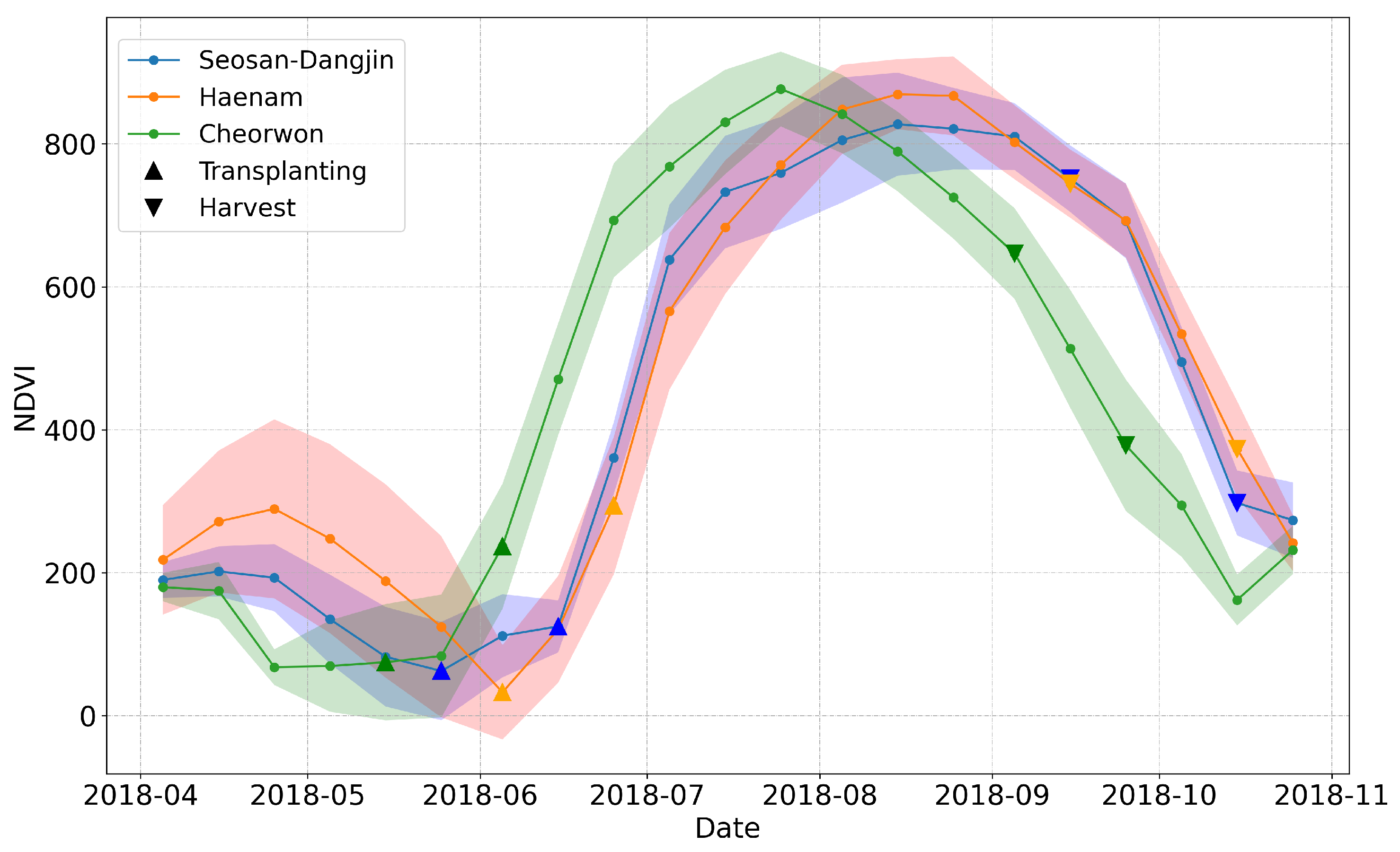
Rice paddies are inundated approximately one month before transplanting takes place. However, the start of the inundation period differs from place to place. For instance in the Haenam site, transplanting takes place a bit later in the year. Figure 2 shows the mean values of NDVI for rice paddies in each site.
The faded colored area around each curve illustrates the standard deviation. The differences in the growth of paddy rice among the sites are evident. The high standard deviation values for the months of April and May on the Haenam curve can be explained by the fact that certain parcels go through one winter and one summer cultivation within the same year. This results in a slight delay of the transplanting period, as it is indicated by the orange curve in Figure 2.
Furthermore, the period in which transplanting can take place is enclosed within the up-pointing triangles at the beginning of each NDVI curve. Respectively, the down-pointing triangles at the end of each curve correspond to the periods in which harvesting can occur. Therefore, in order to create a generalized and robust rice classification model that is not subject to the aforementioned region-based differences, the feature space is truncated to include acquisitions starting from June onward, for all sites.
After pre-processing all available Sentinel-2 images to Level-2A products, using the Sen2Cor software, we selected the cloud-free instances based on the percentage of cloud coverage according to the generated Scene Classification [42]. The cloud mask produced from the Scene Classification product, included the classes of high probability clouds, medium probability clouds, cirrus, snow and cloud shadows. Then, only the images with cloud coverage less than 70% over the site were included in the feature space. The relatively cloud-free Sentinel-2 datasets used for each site, covering June to October of 2018, amounted to 16 images for Seosan-Dangjin (128 GB), 13 images for Haenam (130 GB) and 19 images for Cheorwon (90 GB).
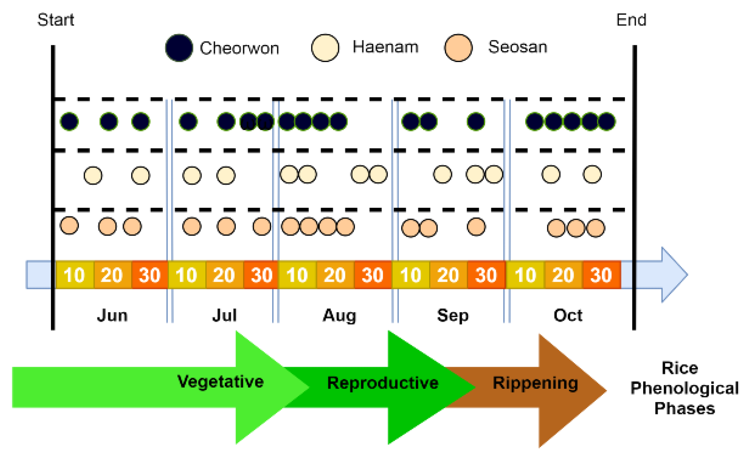
Figure 3 indicates the acquisition dates for the selected Sentinel-2 images for all three sites. These images, along with the generated Vegetation Indices (VIs), construct the Sentinel-2 component of the feature space.

2.2.1. Sentinel-1 Data

A time-series of Sentinel-1 images was acquired between the dates 1 June 2018–31 October 2018. Specifically, we used the Level 1 Ground Range Detected (GRD) products in Interferometric Wide (IW) swath mode. The IW mode acquires data with a 250 km swath at 5 m by 20 m spatial resolution. The pre-processing of Sentinel-1 data included (i) clipping to the area of interest, (ii) radiometric calibration, (iii) speckle filtering using the Lee filter, (iv) terrain correction using Shuttle Radar Topography Mission (SRTM) 10-m and (v) conversion of backscatter coefficient ( σ 0 ) into decibels (dB). The steps are shown in Figure 4. The VV and VH bascatter coefficient time-series are sampled with a fixed 10-day step, averaging the values in each 10-day window. This is done in order to slightly reduce the dimensionality of the Sentinel-1 component of the feature space.

2.2.2. Sentinel-2 Data

For this study, a time-series of Sentinel-2 MSI scenes were acquired for the period June to October 2018. The Sentinel-2 images consist of 13 spectral bands at 10, 20 and 60 m of spatial resolution. The 60 m resolution bands, namely B01, B09 and B10, have not been utilized. Furthermore, the images have been atmospherically corrected, transforming them from Top-Of-Atmosphere (TOA) Level 1C products to Bottom-Of-Atmosphere (BOA) Level 2A products, using the Sen2Cor software [43]. The data were then re-sampled to 10 m spatial resolution, re-projected and clipped over the areas of interest.
Furthermore, three vegetation indices were computed to enhance the feature space, namely the Normalized Difference Vegetation Index (NDVI) (Equation (1)), the Normalized Difference Water Index (NDWI) proposed by Gao et al. (1996) (Equation (2)) and the Plant Senescence Reflectance Index (PSRI) (Equation (3)) [44,45,46]. The NDVI and NDWI indices have been extensively used in the EO-based crop classification literature, as they are good indicators of the biomass and water content of crops. On the other hand, PSRI is particularly sensitive to the crops’ senescence phase [25,47,48,49,50,51].
n d v i = n i r r e d n i r + r e d
n d w i = n i r s w i r n i r + s w i r
p s r i = r e d b l u e r e d _ e d g e

2.3. Labeled Data

This study focuses on generating pseudo-labels, using unsupervised learning, in order to train a distributed RF classifier. Nevertheless, labeled sets have been both acquired and generated to (a) select the optimal clustering for pseudo-labels that will form the training set (Section 3.2), (b) fine-tune the model for nationwide generalization (Section 3.2) and (c) test the model generalization (Section 4).
Level-3 land cover maps were used as an initial reference point for generating the labeled data, as made available from the Korean Ministry of Environment (KME). The Level-3 land cover maps are generated using Very High Resolution (VHR) satellite imagery (KOMPSAT-2 and IKONOS) and aerial ortho-photos from one or two years [21]. The map objects are 3-m wide for linear elements and 100 m2 for plane elements and therefore the spatial resolution is comparable to the corresponding resolution of the Sentinel data. However, the maps are not updated every single year. Furthermore, it was deduced that they tend to be unreliable and subject to significant errors with respect to both object geometries and the land cover labeling. Nonetheless, they were an adequate starting point for our labeling process.
The labeled data generated in this study have been derived from a Sentinel-1 and Sentinel-2 based photo-interpretation. The labeling process refers to the identification of rice and non-rice pixels and it was applied to all three study sites, for the inspection year of 2018. The method has been based on the most recent Level-3 land cover map for each respective site, which were then appropriately corrected to be compliant to the year of inspection. To this end, the first step was to utilize a change detection method, as published in [52], to update the available Level-3 land cover maps for each site. This was done by identifying large changes on rice objects between the year of the land cover map production and the year of inspection. Those instances were later removed from the rice class of the updated maps.
Consequently, two different experts conducted blind photo-interpretation using multi-temporal Sentinel-1 and Sentinel-2 images and the updated Level-3 land cover maps as a reference. Each of the first two interpreters independently assigned labels to approximately 5–10% of each site. Then, a third interpreter determined the final labels by making an ultimate decision on the disagreements of the first two. The samples were evenly distributed in space and thus representative of the entire site to ensure reliable model optimization and classification assessment. Additionally, the samples were taken from diverse landscapes including agriculture, water, forest and urban classes. The locations of the photo-interpreted samples are presented in Figure S1.
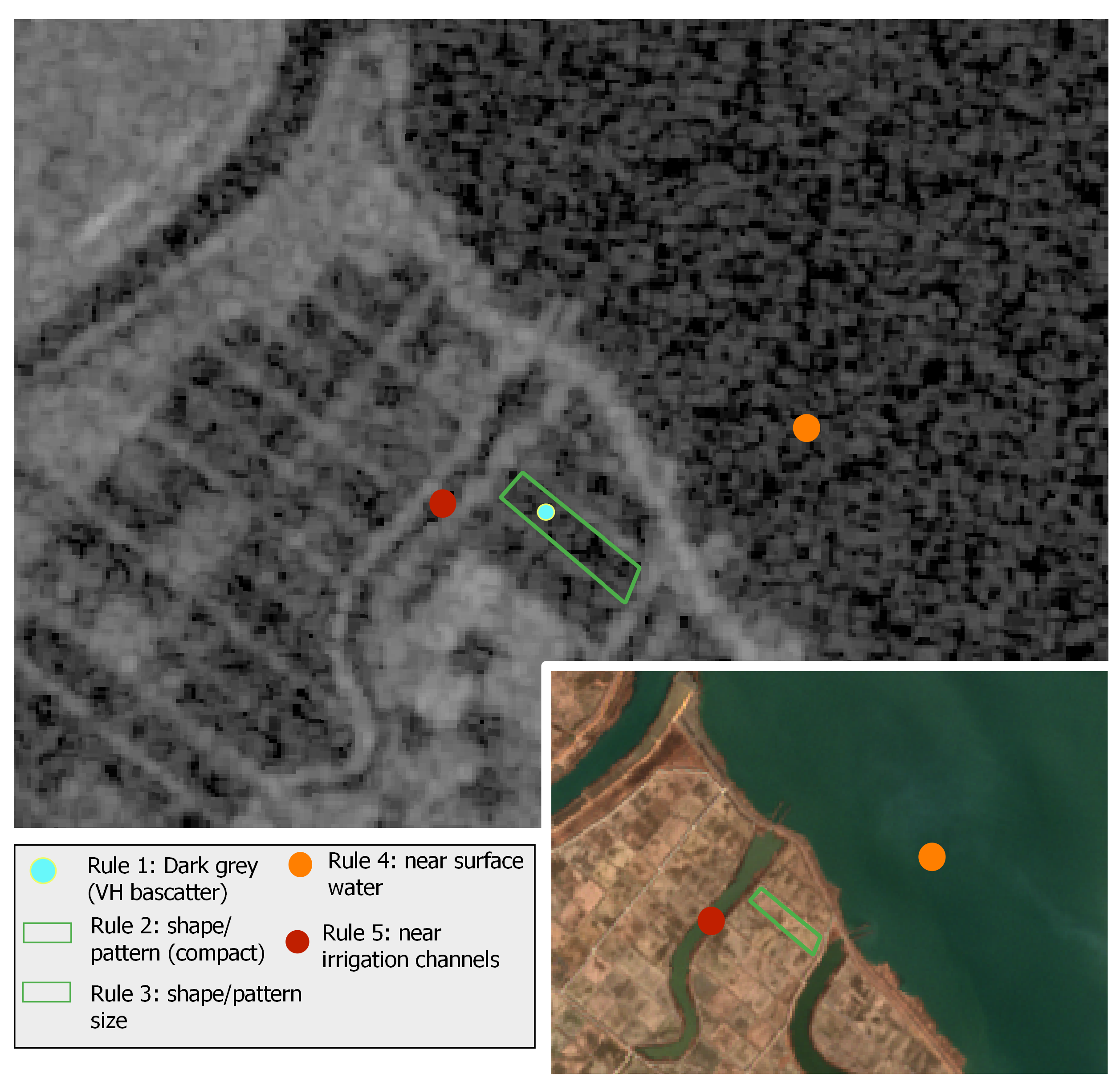
The inundation and transplanting periods for paddy rice differ among the study areas. Specifically, in Cheorwon the inundation starts in the mid-late April, while in Seosan-Dangjin in the end of April and in Haenam in the middle of May. Therefore, the photo-interpretation analysis included Sentinel-1 and Sentinel-2 data starting from the month of April. The sensitivity of Sentinel-1 data to water has been primarily used to identify the inundated areas before the start of the transplanting phase. Low backscatter coefficient values, revealing water content, and the corresponding geometric patterns of fields have served as a first indication to separate and label the rice paddies [28]. Figure 5 shows the photo-interpretation rules used in the first step of the labeling process.
Rules 1–3 had to be satisfied, while rules 4 & 5 served as an additional indication for the labeling of rice paddies. To be noted that in certain cases, and especially due to the size of a paddy rice or its narrow shape (e.g., terrace paddy), it was difficult to extract reliable information on existing inundation patterns using solely Sentinel-1 data. To overcome this problem, an analysis of NDWI multi-temporal profiles was additionally carried out for candidate rice paddies that had satisfied several or all of rules 2–5, but not rule 1. Actually, in cases that NDWI was found smaller than 0.2 before transplanting, in the specific parcel was assigned the non-rice label, otherwise the decision process was moving to the next step that made use of Sentinel-2 multi-temporal photo-interpretation keys. An indicative example is illustrated in Figure 6.
The interpretation of the time-series of Sentinel-2 true color and false color (B08-B04-B03) composites has proven to be particularly useful in examining whether or not a parcel complies with the different phenological stages of rice. In the end, the examination of NDVI and NDWI multi-temporal signatures were used to guide the final decision of the photo-interpreter. Their decision was dictated by the fact that NDWI gets higher values before the transplanting period and starts lessening thereafter. On the other hand, NDVI exhibits the inverse phenomenon, as it increases after the transplanting period, reaching its peak values at the end of flowering, when it starts decreasing again as rice enters in its ripening phase (Figure 6). This procedure was applied in all three study sites. The generated labeled sets for the Seosan-Dangjin, Haenam and Cheorwon sites included 1,675,632 non-rice and 1,287,183 rice pixels, 2,944,147 non-rice and 892,141 rice pixels and 1,137,195 non-rice and 195,942 rice pixels, respectively.
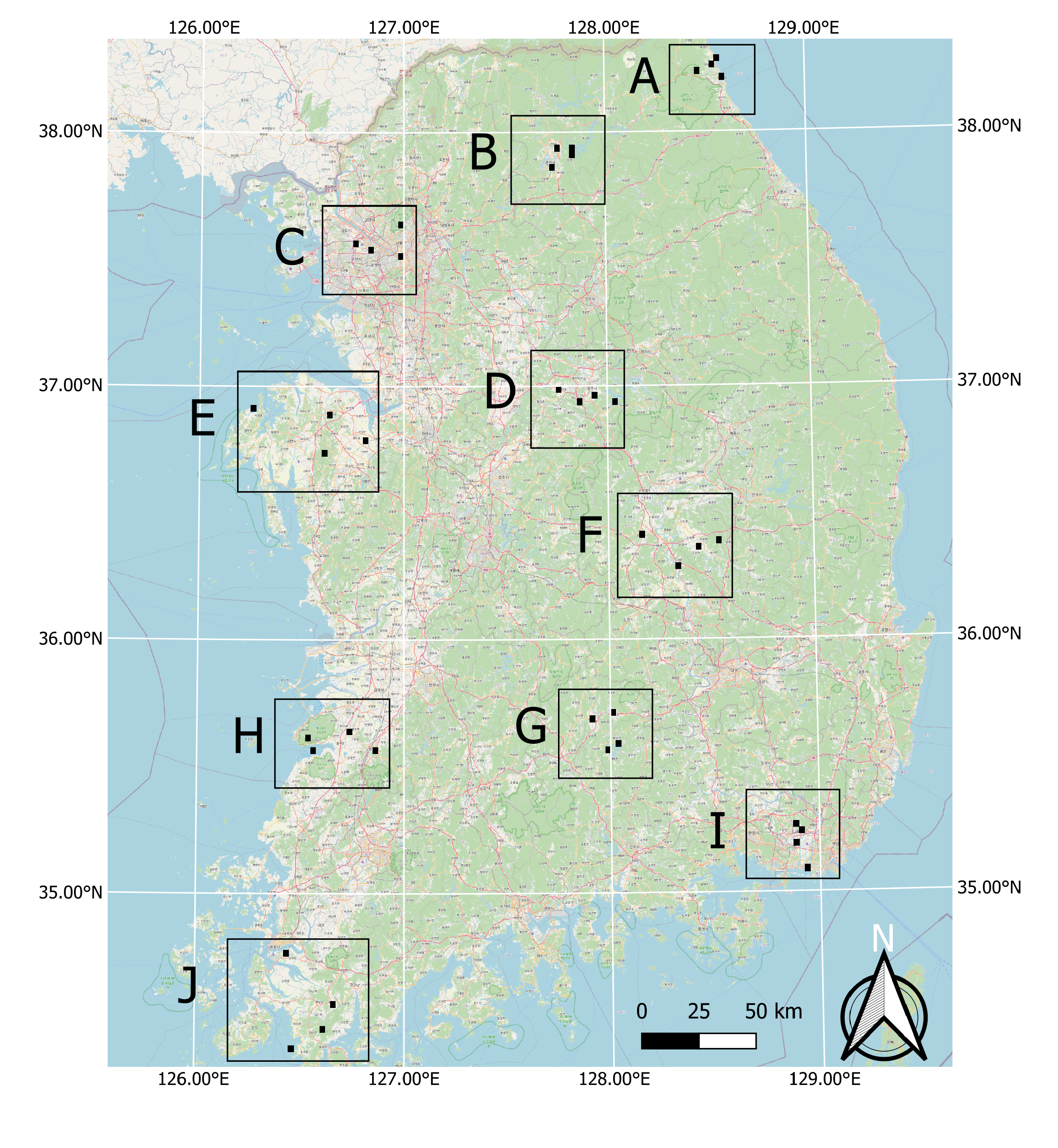
Finally, in order to further test the success in the generalization of the model, its transferability and robust applicability in different agro-climatic zones over the entire country, the labeled set created by the authors of [21] was additionally included and used in this study (Figure 7). For this, the authors have identified ten evenly distributed sites in South Korea that fall into ten different agro-climatic zones according to [30]. Each site includes four plots in agricultural, urban, forest and water abundant landscapes. The size of the plots ranged from 6 to 6.5 km2. By applying a photo-interpretation study, the necessary test data were produced based on the existing level-3 land cover maps that were updated to reflect the 2018 reality. This was done using visual interpretation and cross-validation with the employment of three independent interpreters, who were assisted by Google Earth and domestic street view data (https://map.kakao.com; https://map.naver.com).

3. Methods

3.1. Sentinel-2 Time-Series Interpolation

The cloud covered instances in the Sentinel-2 time-series, which were masked out, are represented as null values in the feature space. We applied linear interpolation in order to fill in these gaps. Due to the large volume of the data, this method was implemented in PySpark and processed in the HPDA. Since there is not any ready-to-use function to interpolate a PySpark Dataframe, this interpolation method was developed from scratch. This allowed for the mass processing of the time-series, efficiently filling in the missing values of large datasets.
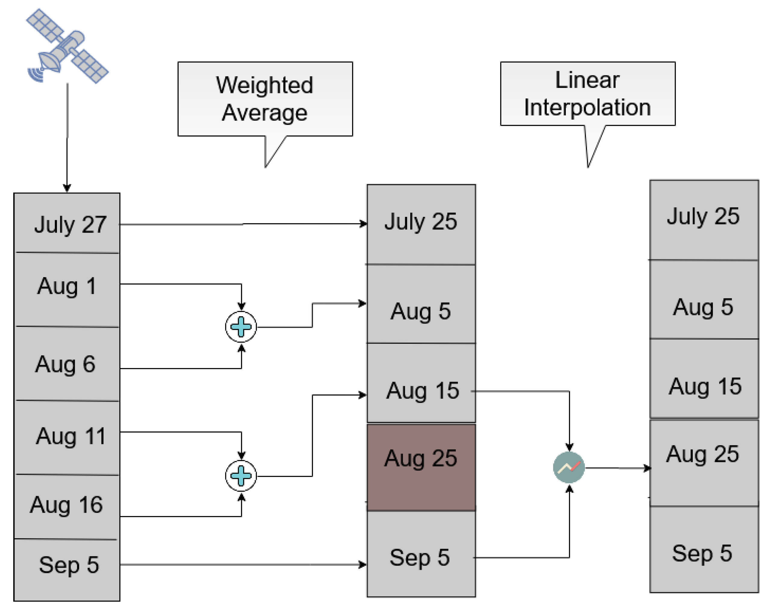
Then, and in order to avoid possible temporal gaps between the available acquisitions, we transformed the Sentinel-2 feature space to a time-series of fixed step, generating values that represent the 5th, 15th and 25th day of each month. In order to do this, a workflow of two separate interpolation methods was followed.
Initially, the method illustrated in Figure 8 examines the time windows between the 1st and the 10th, the 11th and the 20th and the 21st until the end of each month. A weighted average interpolation is applied to the acquisitions that fall within each window and it then constructs part of the fixed-step time-series. However, it is likely that there are not any observations within a specific window, resulting in the absence of features for the corresponding temporal instance. In order to fill these remaining temporal gaps, linear interpolation was applied between the previous and next available fixed temporal instances.

3.2. Pseudo-Labeling

In an attempt to address the common issue of ground truth data scarcity, we examined a pseudo-labeling approach to generate labeled data for training. This can be done using only a small amount of ground truth data (see Section 5). The pseudo-labels were generated using a distributed k-means classifier, employing as input the time-series of the vegetation indices (NDVI, NDWI, PSRI) for the months of June and July.
K-means is one of the simplest and most popular unsupervised machine learning algorithms [53,54,55,56]. The algorithm aims to cluster the data into k groups, where the variable k is specified by the user. At the beginning, k different clusters are created, using k randomly generated candidates. Then every entity is assigned to the nearest cluster based on their features. In the next step, the entities are reassigned to the nearest cluster that is now represented from the mean value of the entities that belonged to it from the previous step. The algorithm keeps iterating until the assignment of data points to clusters remains unchanged. The outputs of the algorithm are the means of the k clusters (centroids), as well as the labels for each sample, which are then used as training data.
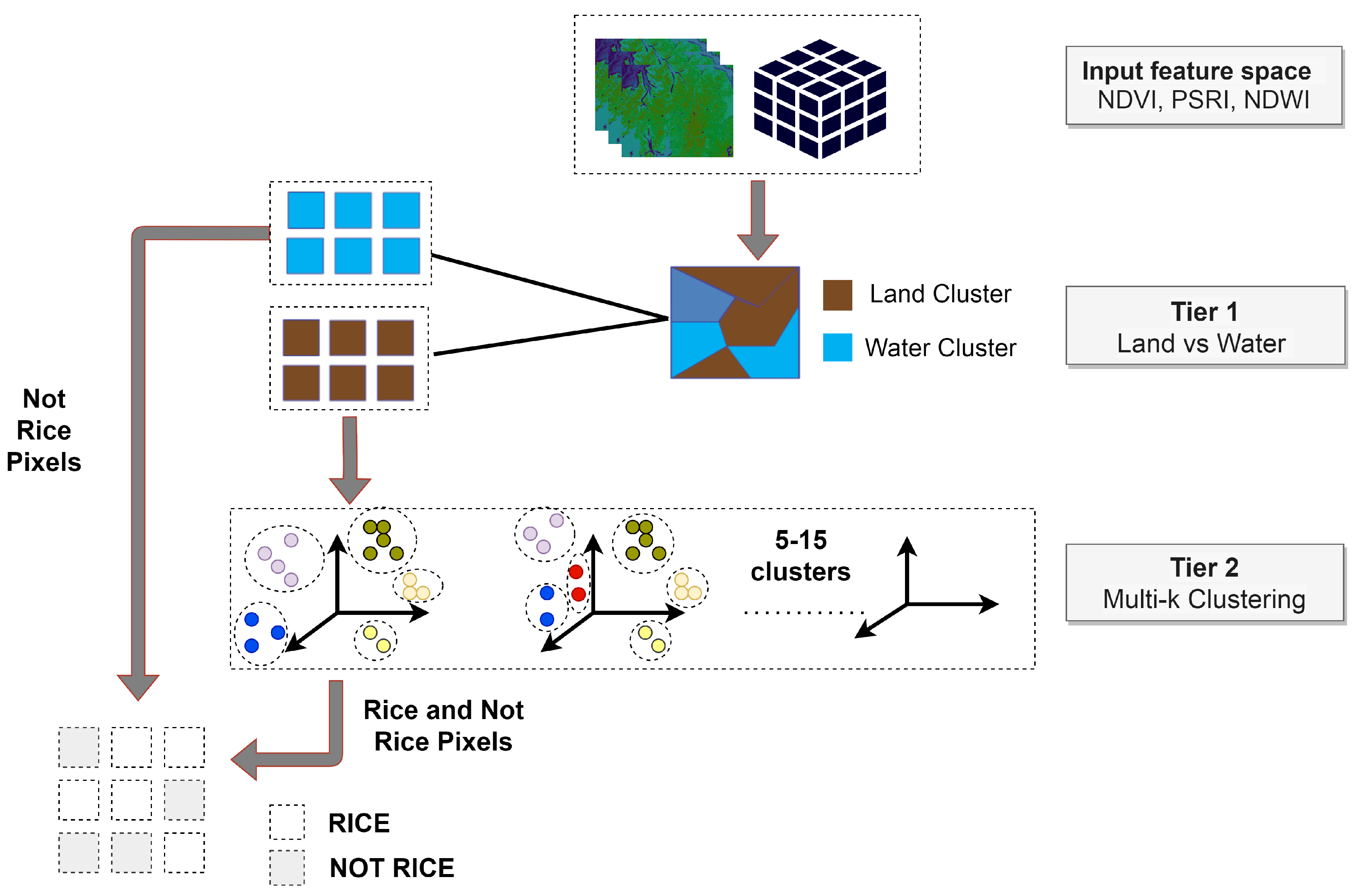
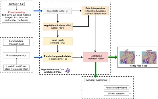
In our approach and due to the large volume of data the distributed k-means version of the Pyspark API was used. First, an execution of k-means is performed with only two clusters (k = 2), separating land from water. Having extracted the land pixels, a second-level clustering for multiple k values (5–15) takes place (Figure 9).
Each pixel is assigned to a different cluster. However, there is no further information about the land cover that each cluster represents. Thus, a method to identify the rice cluster for all individual clusterings (for k = 5–15) is required. This is achieved by the Mean Squared Error (MSE) between the centroid of each cluster and the mean time-series signature of the rice class, as extracted from the labeled set (Section 2.3).
Once the rice cluster has been identified for each individual run, the precision and recall for this cluster is calculated against the labeled set. This is the only instance when labeled data are utilized in the classification process. The clustering with the best precision and recall combination is selected, and these extracted rice labels are then used for training the RF (Section 3.4). The optimal combination of precision and recall is shown in Section 4.

3.3. Model Performance Evaluation

In this study, four metrics were used to evaluate the performance of the paddy rice classification model and that is the precision, recall, kappa coefficient and F1 score. The aforementioned metrics are derived from the confusion matrix between the model predictions and the ground truth stemming from the validation and test sets [57]. Precision (Equation (4)) reveals the actual number of pixels that the model has predicted correctly, whereas recall (Equation (5)) denotes the proportion of the correctly classified pixels against the total number of pixels for a particular class [58]. In addition, the kappa coefficient (Equation (7)) identifies the difference between the actual classification and a random classifier; therefore removing the component of random agreement [59]. Finally, classification performance is also evaluated using the F1 score (Equation (6)), which is the harmonic mean of precision and recall [60].
P r e c i s i o n = T P T P + F P
R e c a l l = T P T P + F N
F 1 s c o r e = 2 2 · T P + F P + F N
K a p p a = p o p e 1 p e
where TP is the number of True Positive instances, FP the number of False Positive, FN the number of False Negative, p o is the relative observed agreement between the ground truth and the prediction, and p e is the hypothetical probability of chance agreement.

3.4. Supervised Classification Using Pseudo-Labels

The Random Forest (RF) is an ensemble classifier based on the decision tree model. The training data are split into multiple different subsets, using the bootstrap method, and each subset creates a new decision tree. Finally, a forest is constructed from the different decision trees and predictions are made through majority voting [61].
In this study, a distributed RF implementation was employed in order to address the great complexity that comes with the large scale application of paddy rice classification. The algorithm utilized MLLib, a library of Apache SPARK, in which many of the optimizations are based upon Google’s PLANET project [62]. First of all, each tree of the RF ensemble is trained independently, thus multiple trees can be trained simultaneously on different nodes. Further, MLLib enables the parallelization on each single tree of the ensemble, allowing for the concurrent training of multiple sub-trees. The optimal number of these sub-trees is optimized on each iteration of the algorithm, depending on memory constraints [63].
MLLib optimizes the algorithm using techniques to avoid unnecessary parses on data. For example, splits for every tree node of the same level are computed simultaneously with only one pass over the data, rather than one pass for each node individually. For the best split computation, features are separated into bins, which are then used to calculate useful statistics for the splitting. These bins are precomputed for each of the instances, thereby saving computational time.
The distributed RF classification pipeline has been deployed on an HPDA environment, which gives the ability to train a model in significantly less time than a conventional machine. In this study, we used the Cray-Urika-GX of the High-Performance Computing Center Stuttgart (HLRS). The Cray-Urika-GX comprises 41 nodes, with 512GB of RAM and 2TB of disk capacity each. Each node is composed of 2 Intel BDW 18-Core (2.1 GHz) processors. For this work, up to 16 nodes were utilized for the experiments, making it possible to explore multiple parameterizations of the RF model in a short amount of time.
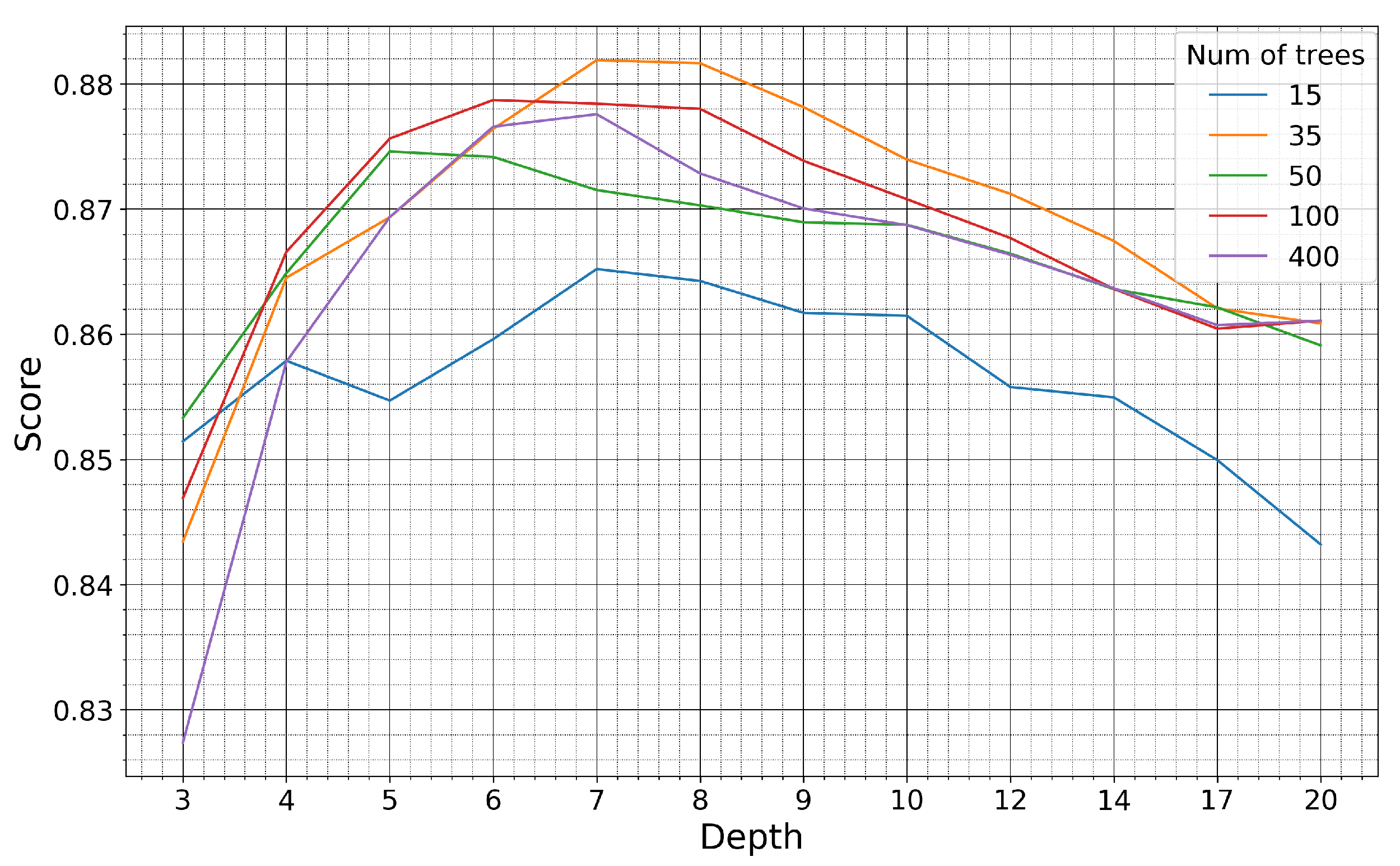
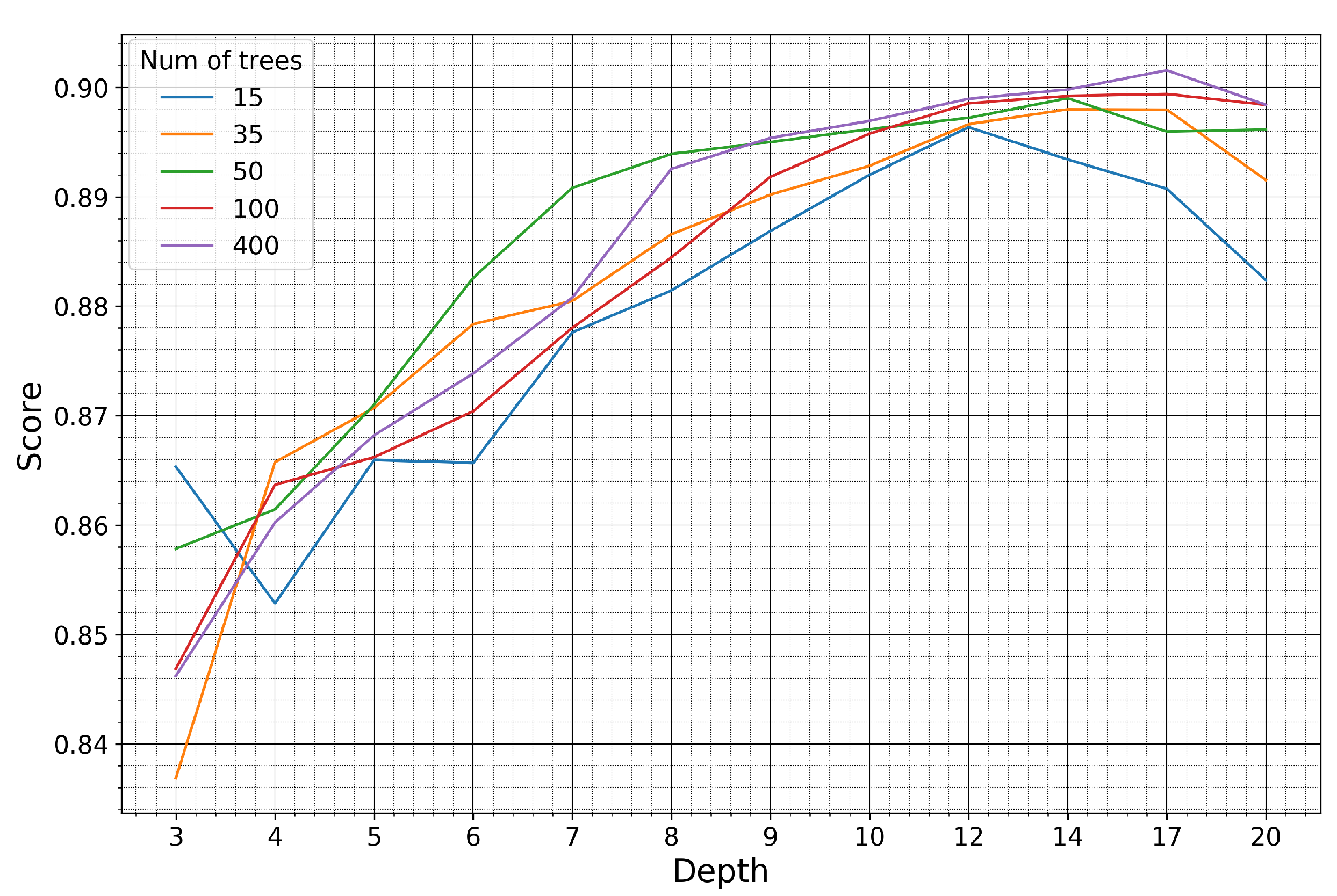
The model was trained on the pseudo-labels generated in the Seosan-Dangjin site. The hyperpameters were optimized using half of the labeled samples for the Haenam and Cheorwon sites (validation set). The other half was used for testing the performance of the optimized model, as presented in Section 4 and Section 5 (test set). Figure 10 and Figure 11 demonstrate how the kappa coefficient responds to the depth size and number of trees of the RF model.
For the Haenam site, the kappa coefficient increases for larger depth sizes. This is true until the depth parameter becomes equal to 8, after which the kappa coefficient slightly decreases. For the Cheorwon site, the kappa coefficient increases almost linearly with an increasing depth, until it reaches a plateau for depth values larger than 12.
The response of the kappa coefficient for a varying number of trees, in combination with several depth values, was observed for tens of experiments in the range 10–400. In Figure 10 and Figure 11, we depict five indicative cases that fully describe the relevant response of the RF. For 15 trees, the kappa values for both sites are less than optimal, although satisfactory. For 35 or more trees, however, the performance stabilizes and displays marginal differences for all different depth values.
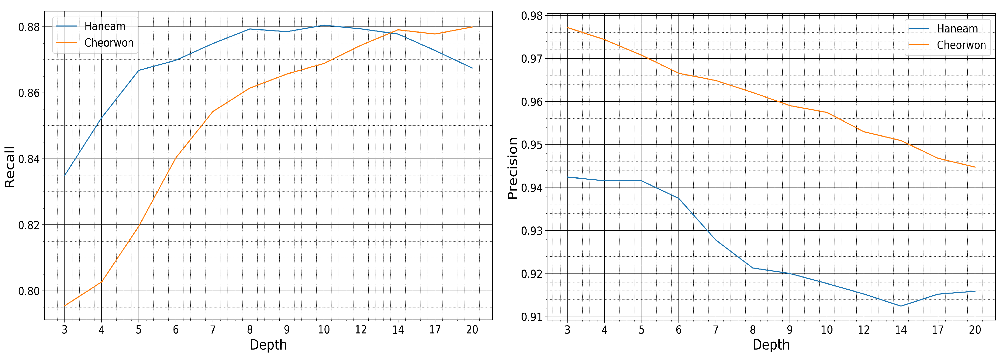
The value of choice for the number of trees parameter was 50, as a trade-off between accuracy and computational complexity. In Figure 12 is displayed the relative performance between the two sites for increasing depth size. The precision and recall evolution plots are run for a fixed number of trees equal to 50.
It is observed that for increasing depth values, the scores decrease for precision and increase for recall, as expected. However, the performance for the Haenam site and for depth sizes larger than 12 appears to lose not only in precision but also in recall. This indicates model overfitting. This phenomenon is evident in the Haenam site mostly because the transplanting period commences later in the year. Starting the time-series that makes up the feature space from June, and not earlier, partly resolved the issue. Nonetheless, large depth sizes capture more of the Seosan-Dangjin site particularities that has a negative impact in the generalization of the model to areas with different characteristics, such as the Haenam site. For this reason the depth parameter used was set to 12.

4. Results

4.1. K-Means Clustering

As mentioned in Section 3.2, we perform dynamic clustering for multiple k values to generate pseudo-labels. The RF model was then trained on the pseudo-labels that come from the Seosan-Dangjin site. Nevertheless, the k-means algorithm was executed for all three study sites. This was done in order to showcase the robustness of the pseudo-labeling method, while at the same time generate local pseudo-labels for training individual RF models for the Haenam and Cheorwon sites. The locally trained models for these two sites are then compared to the predictions of the Seosan-Dangjin site model to demonstrate the success of the generalization (Section 5).
In Table 2 is shown the precision, recall, F1-score and the optimal number of clusters for the k-means clustering in each of the sites. It can be observed that for all sites the performance scores are satisfactory for both the rice and non-rice classes.
The implemented unsupervised classification method is dynamic, as it tries out multiple k values and selects the most appropriate. It is also robust, as it returns predictions of comparable accuracy for different areas of application. The best k is selected to appropriately balance precision and recall. This trade-off combination of the two metrics was defined by observing the results of multiple experiments.
The experiments were evaluated using the RF accuracy metrics, therefore examining the quality of the pseudo-labels in their capacity as training samples. The experiments revealed particular sensitivity to the recall metric. Experiments of recall smaller than 85% yielded sub-optimal RF classification results, as the training set was not adequately representative. Therefore, the first condition for selecting the best clustering was that recall must be larger than 85%. Precision is also very important, securing the minimization of noise in the pseudo-labels. Thus the second condition was for precision to be larger than 90%. If both conditions were satisfied for more than one clustering, we chose the one with the highest F1-score.

4.2. Model Performance for Varying Training Set Size

Figure 13 shows how the precision, recall and F-1 score respond to the training set size. The scores were calculated against the labeled data of the Haenam and Cheorwon sites that were not used in fine-tuning the hyperparameters of the generalized model. The training set size on the x-axis refers to the number of samples on which the model was trained. The site comprises 41,645,772 pixels and the different training sets of increasing number of samples are randomly selected.
It is observed that with higher training set sizes the precision slightly decreases, while recall increases. It can also be seen that the performance scores are high even with only a limited number of training data. A model that uses a training set of 0.4 M pixels, including approximately 90,000 rice pixels, reaches near-optimal recall values. The precision and the F1-score get high values even for surprisingly small training sets, e.g., 0.002 M. However, the associated recall value is substantially lower that indicates overfitting, which is expected for such small training sets. The results presented from this point on were trained with roughly 4 M training pixels.

4.3. Feature Importance

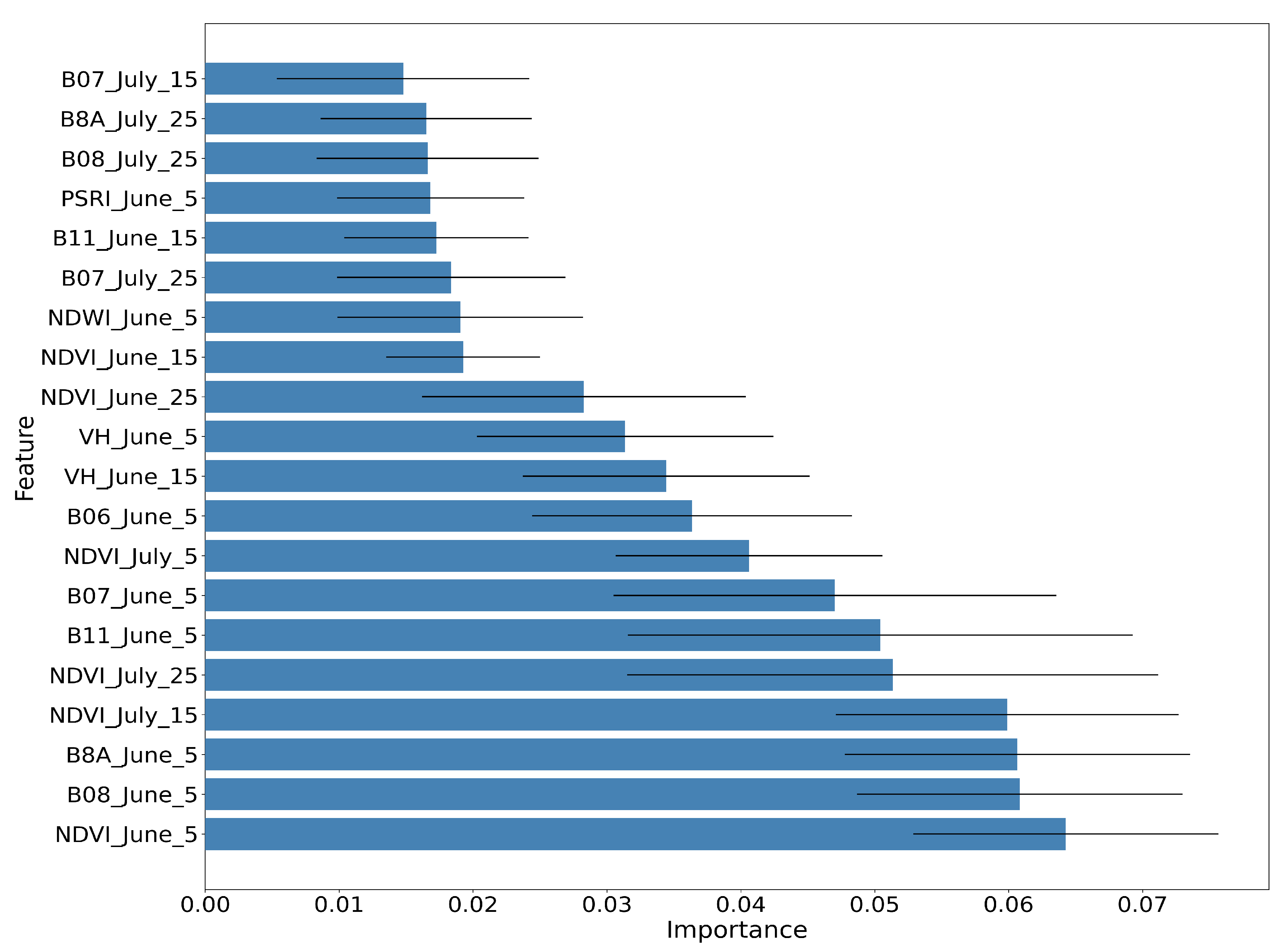
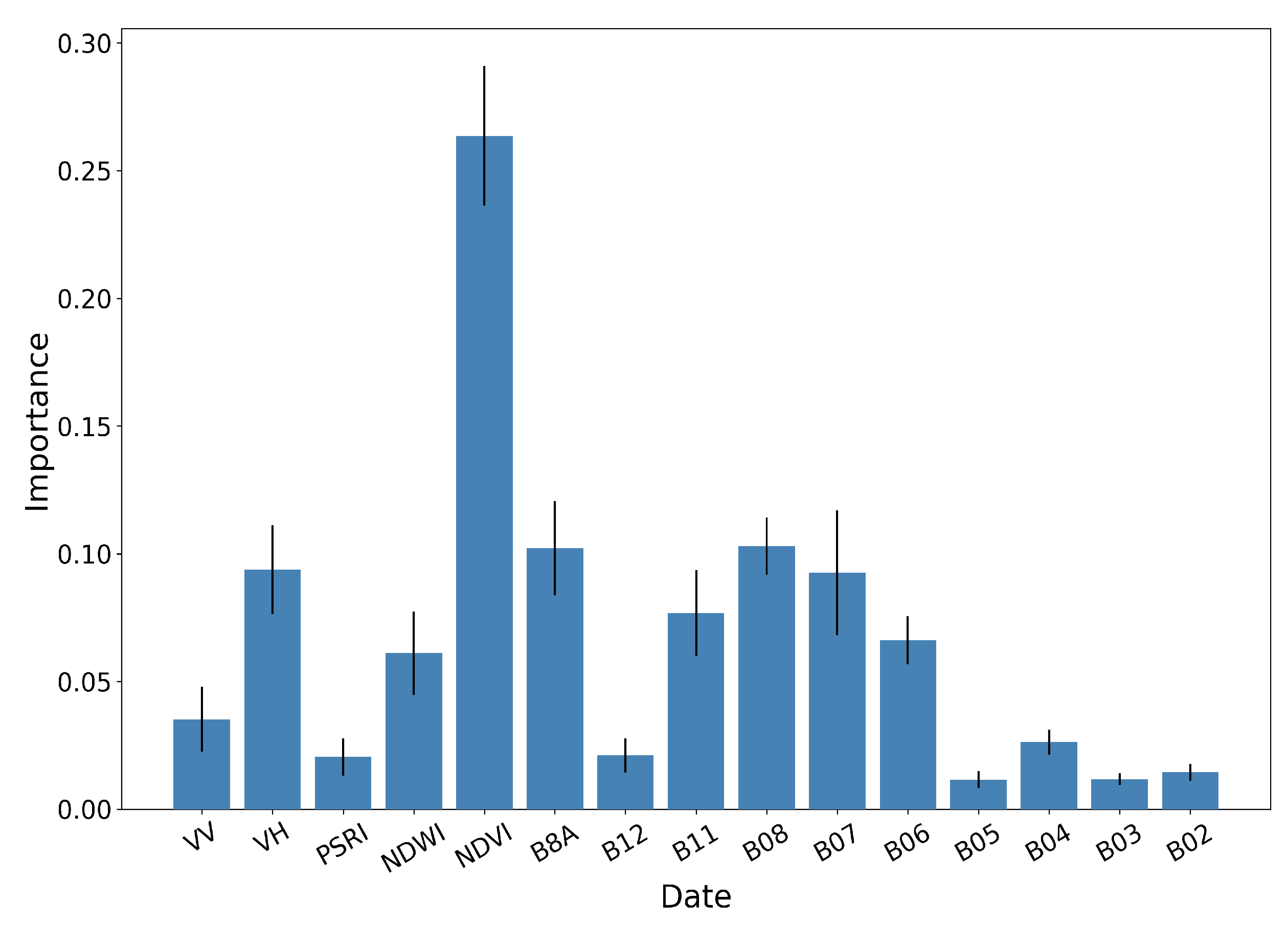
Figure 14, Figure 15 and Figure 16 show the RF importances for the optimized model of 50 trees and depth equal to 12.
The importance values have been averaged for running the same algorithm 10 times with the same hyper-parameters using 10 different random seeds. Figure 14 shows the RF importances of the top 20 ranked features, which include the Sentinel-2 bands B08, B8A, B11, B07 and B06, all vegetation indices (NDVI, NDWI, PSRI) and the Sentinel-1 backscatter coefficients VH and VV.
It is observed that bands B08 and B08A (NIR) and the vegetation index NDVI for 5 June, along with the NDVI index for July15 and July25, are the most important features for the paddy rice classification. The Sentinel-1 features (VH June15 and VH June5) appear in the tenth and eleventh position, with significant contribution.
Figure 15 illustrates the aggregated importance values for the different feature categories. NDVI appears to be by far the most important, followed by the red-edge and NIR bands of Sentinel-2 and the VH backscatter coefficient of Sentinel-1. In the same fashion, Figure 16 aggregates the importance values with respect to time. The June5 instance appears to dominate the importances. This is expected, as by that date the rice fields are fully inundated, allowing for their discrimination among other crop types.

4.4. Accuracy Evolution

Figure 17 shows the evolution of precision and recall for incrementally larger feature spaces. The four different feature spaces, for which the classification performance is compared, are composed of features from the first acquisition of June until the last acquisitions of July, August, September and October, respectively. As expected, richer feature spaces achieve both better recall and precision. Nonetheless, it can be concluded that near-optimal performance is achieved early in the year, allowing for the timely decision making on food security matters. The model generalizes successfully even with short time-series that merely include the months of June and July.
Table 3 shows the total predicted paddy rice area for each of the three sites, compared with the official KOSIS statistics for the year 2018. The last column of the table shows the deviation of the predicted area against the KOSIS equivalent, which is minimal for all sites.

4.5. Model Generalization

In order to evaluate the model performance at national scale, we have used 10 labeled sites in different agro-climatic zones across the country. Each site consists of four plots of diverse landscape characteristics, as described in Section 2.3. Table 4 shows the total accuracy and kappa coefficient of the optimized model for each different plot of the test set.
The authors in [21] have evaluated the performance of multiple deep learning models for paddy rice mapping against this particular test set. The values in light blue and light orange show the instances for which this study’s model performs better or worse than the top performing model in [21], respectively. The improvements when using this study’s model range from 0.5% to 10% (kappa for D), while the decreases in accuracy range from 0.5% to 4% (Accuracy for I: Agriculture). This study’s model achieves a total kappa coefficient of 0.87; while the overall precision and recall of the rice class is 88.91% and 88.19%, respectively. The results are comparable to the corresponding test scores for the Haenam and Cheorwon sites. The predicted paddy rice maps for all 40 test plots can be found in Figure S4 of the Supplementary Material.
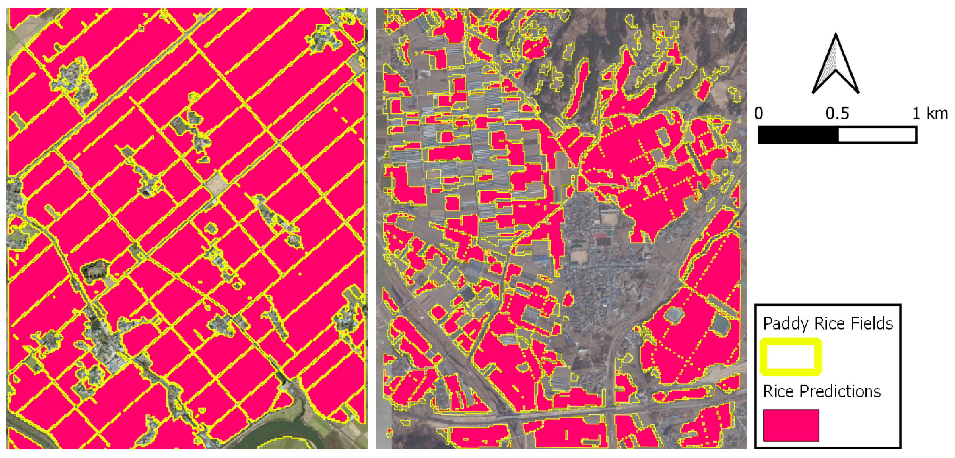
Figure 18 shows a good (E: Agriculture) and a bad (G: Agriculture) example of the predicted rice maps. In plot E, where the rice paddies are spatially continuous there are only few misclassifications. On the other hand, plot G is characterized by fragmented, small and narrow rice parcels, yielding some errors as a result of mixed pixels.

5. Discussion

It should be noted that using unsupervised classification for generating training data (pseudo-labels) allows for producing samples over very large areas. In the alternative case of using ground truth data from field visits, the samples would have been limited in number, fragmented in space and thus potentially less representative.
Despite the high accuracy of the k-means clustering, some rice instances are still mislabeled. However, these instances do not belong to a single cluster, yet they are split among other robust clusters. This suggests that there is not any specific pattern of rice paddy that is left out. Moreover, RF successfully manages to correctly classify a significant number of those mislabeled pseudo-labels. Specifically, the RF precision and recall scores for the rice class, when tested in the Seosan-Dangjin site, were 98.66% and 93.99%; offering an improvement over the pseudo-labels of +1.65% and +2.17%, respectively.
It is the excellent performance of unsupervised classification that allows for the generation of high quality labeled data to train an RF model. The success of clustering can be attributed to the nature of the target. Paddy rice is a distinctive crop type, mainly due to its inundation period, constituting it a particularly easy target to discriminate. This can be further supported by Figure 16 that shows that features from the June5 instance are by far the most important.
Another important characteristic is the abundance of paddy rice in the study sites. For the year of inspection, paddy rice made up 78.2% of the agricultural land of the Dangjin region, 71% of the Seosan region, 54.19% of the Haenam region and 74.6% of the Cheorwon region. Paddy rice is the most dominant cultivation in the areas of inspection, which further enhances the performance of unsupervised classification. Additionally, South Korea is characterized by spatially continuous rice fields with minimal fragmentation. This again contributes to realizing satisfactory clustering results.
Therefore, it could be argued that for binary classification problems, which share similar characteristics, the implemented pseudo-labeling approach can be applicable. In fact, pseudo-labeling constitutes the overall methodology transferable. The three study sites of different agro-climatic conditions, geomorphological characteristics and land cover abundances, yielded excellent and comparable results; showcasing the robustness of the method. The idea of pseudo-labeling for crop classification could be even extended to multi-class scenarios. Multi-crop classification problems could be reduced to multiple OnevsAll binary classifiers, such as the one implemented in this work.
Finally, it should be noted that this approach can be employed even in cases that there is no available labeled data, using the photo-interpretation approach suggested in Section 2.3. This way one can annotate a very small amount of rice and non-rice pixels to then use for choosing the best k value for the unsupervised classifier. Table 5 presents the F1 scores for multiple k-means classifications in the Seosan-Dangjin site, calculated against a varying size of the photo-interpreted set of samples. Each experiment is evaluated against a spatially continuous subset of the labeled set across the Seosan-Dangjin site, which includes at least 5000 pixels. Figure S2 depicts the locations of the seven sites (Site id 1–7) of Table 5. Site id 8 refers to the entire labeled set for the Seosan-Dangjin site (Figure S1).
It is observed that for all eight experiments, the models with k [ 6 , 9 ] exhibit the best performance, with marginal differences in their F-1 scores (<1%). More specifically though, the model with k = 7 achieves the best performance for all experiments, regardless of the size of the labeled set used. This indicates the potential for easily generating confined labels through visual interpretation that is solely based on freely available earth observations (Sentinel-1 and Sentinel-2 data).
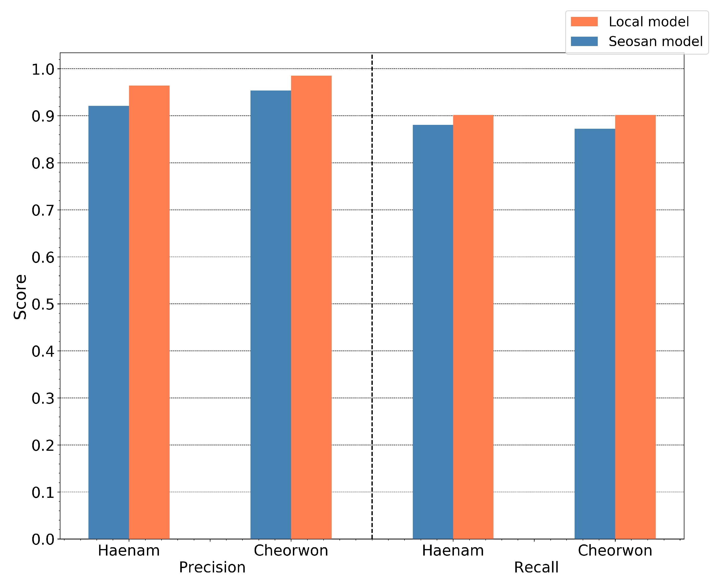
To further investigate the generalization of the RF model, a comparison analysis was conducted between the performance of the transferred model, from the reference site of Seosan-Dangjin, and the locally trained models in the Haenam and Cheorwon sites. The latter refer to trained models with locally sampled pseudo-labels (Table 2). Figure 19 shows the precision and recall for both the locally trained models, which have been individually optimized, and the generalized model of the Seosan-Dangjin site. The differences between the local models and transferred model are minimal. Therefore, it could be argued that a single model from only a small region can be applicable to other areas. This is further supported by the results against the test set in Section 4.5.
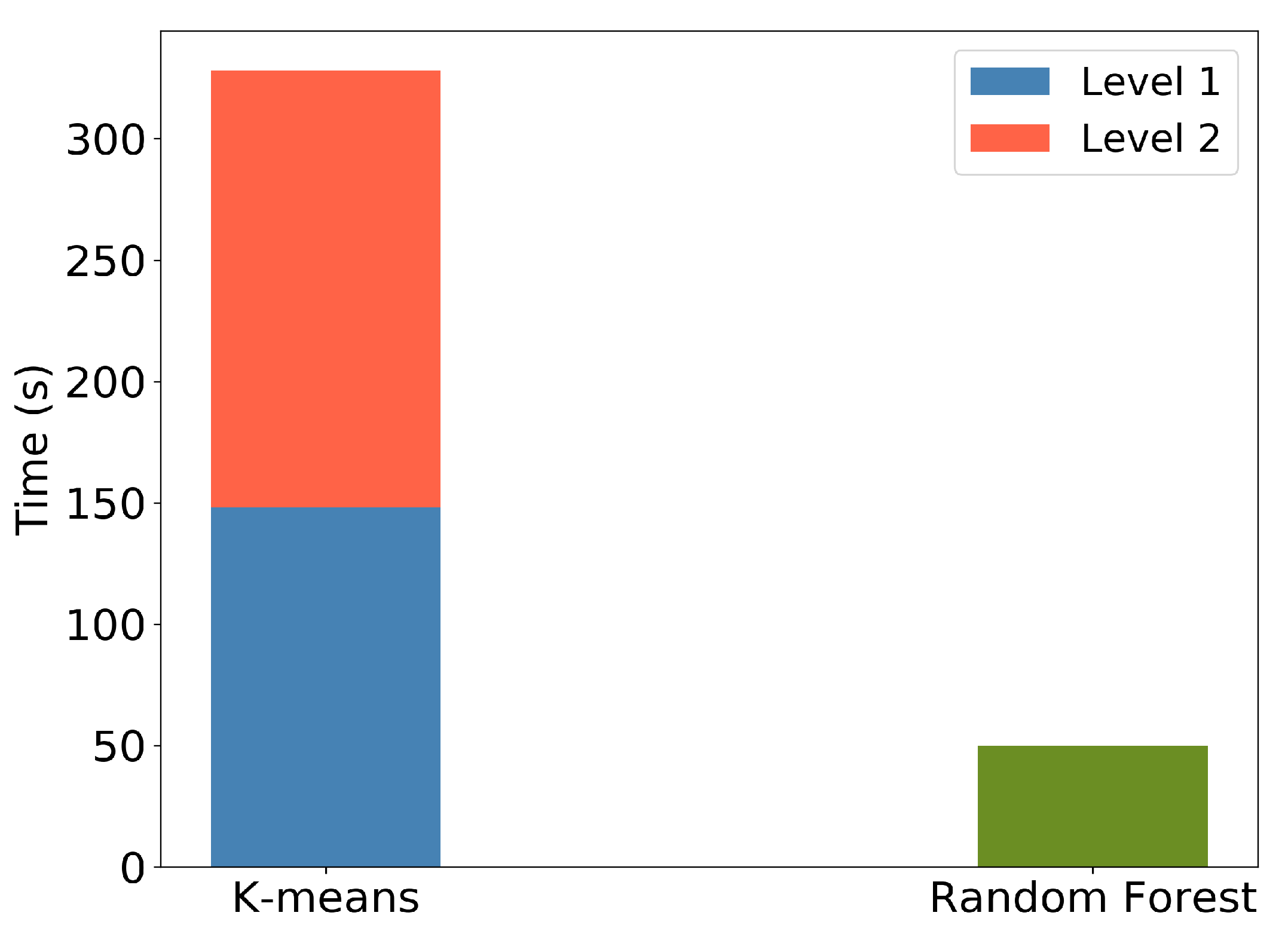
Furthermore, Figure 20 illustrates the execution times for the k-means clustering and RF predictions for the Seosan-Dangjin site. The k-means execution time includes both levels, namely the binary land/water clustering (k = 2) and the succeeding clustering on the land mask (k = 7). Clearly, the RF model inference is significantly more efficient. The computational complexity reduction by not performing k-means clustering in each area is supported by the very good performance of the transferred model when compared to the local ones.
Figure 21 illustrates the RF training time for the Seosan-Dangjin site against an increasing number of employed nodes in the HPDA. The training set used for these measurements comprise roughly 4 M pixels.
Each node is composed of 36 CPUs and 512 GB of memory. It is observed that the training time decreases exponentially with an increasing number of nodes, until it converges to approximately 50 s for more than 12 nodes. Additionally, applying the trained model to the Haenam and Cheorwon sites takes less than one minute for approximately 65 M pixels. Therefore, it would take at most one hour to produce a nationwide rice map for South Korea.

6. Conclusions

A distributed RF classifier that was trained with pseudo-labels on a Sentinel-1 and Sentinel-2 data time-series offered an accurate, generalized and thereby transferable model for high spatial resolution paddy rice mapping. The model was trained in the reference site of Seosan-Dangjin and then fine-tuned for nationwide applicability based on two other sites of diverse characteristics. When tested in these two sites the model achieved more than 88% recall and more than 91% precision scores. The model was further tested on 40 test plots, evenly distributed across South Korea. The results revealed a successful model generalization, with an overall classification accuracy 96.7% and kappa coefficient 0.87. Furthermore, the results were returned early in the year that in turn allows for timely decision making.
The implemented pseudo-labeling method is fully dynamic and requires only a confined set of labeled data. Unsupervised classification alone proved to be effective in accurately classifying paddy rice. However, the exhaustive nature of k-means adds significant computational overhead, when framed in the context of large-scale applications. Nevertheless, it was shown that pseudo-labels can be extracted for only a small area and supervised learning models, such as RF, can generalize well to produce accurate rice maps in other areas. Finally, a distributed implementation of the entire semi-supervised pipeline was used in a HPDA environment to ensure the computational scalability of our approach.
All in all, it could be argued that the implemented paddy rice classification pipeline was designed to be dynamic, site independent and computationally scalable, exploiting exclusively satellite data that are freely available. Accurate, detailed and timely information on the paddy rice extent over large areas is instrumental to the national food security management and decision making.

Supplementary Materials

The following are available online at https://www.mdpi.com/article/10.3390/rs13091769/s1, Figure S1: (1) Labeled maps of Cheorwon (A), Seosan-Dangjin (B) and Haenam (C) produced with photo-interpretation (Section 2.3). Blue color represents the rice class, while yellow the non rice class. (2) Rice maps produced by applying the optimized RF model trained on the Seosan-Dangjin site. Figure S2: Locations of the Seosan-Dangjin labeled subsets used to evaluate k-means clustering experiments in Table 5—Site IDs. Figure S3: Climatic and agro-climatic zones in South Korea’s (modified from [30]). Figure S4: Paddy rice maps produced by applying the optimized RF model on 40 test plots across the country. The locations of sites (a)–(j) can be seen in Figure 7.

Author Contributions

Conceptualization, V.S., A.K., C.K. and I.P.; methodology, V.S. and A.K.; formal analysis, V.S., A.K., C.K., I.P. and V.K.; data curation, V.S. and T.D.; writing—original draft preparation, V.S.; writing—review and editing, A.K., T.D., C.K., I.P. and V.K.; All authors have read and agreed to the published version of the manuscript.

Funding

This work has been supported by the EOPEN project, which has been funded from the European Union’s Horizon 2020 research and innovation programme under grant agreement 776019.

Data Availability Statement

Paddy rice prediction maps for the study sites (i) Seosan and Dangjin, (ii) Haenam and (iii) Cheorwon are available in a publicly accessible repository. If this data is used please cite this publication. The data can be found here: https://github.com/Agri-Hub/rice_map/. Last commit took place 8 days ago. Additional commits will follow.

Acknowledgments

The authors would like to acknowledge the High-Performance Computing Center Stuttgart (HLRS) for providing access to the Cray-Urika-GX High Performance Data Analytics infrastructure. Additionally, the authors would like to thank Hyun-Woo Jo and Woo-Kyun Lee from the eGIS/RS Lab of Korea University for providing the labeled set for testing. Finally, they would also like to thank three anonymous reviewers whose suggestions greatly improved the contents of this paper.

Conflicts of Interest

The authors declare no conflict of interest.

References

  1. Fritz, S.; See, L.; You, L.; Justice, C.; Becker-Reshef, I.; Bydekerke, L.; Cumani, R.; Defourny, P.; Erb, K.H.; Foley, J.; et al. The Need for Improved Maps of Global Cropland. Eos Trans. Am. Geophys. Union 2013, 94, 31–32. [Google Scholar] [CrossRef]
  2. Ban, Y.; Gong, P.; Chandra, G. Global land cover mapping using Earth observation satellite data: Recent progresses and challenges. ISPRS J. Photogramm. Remote Sens. 2015, 1–6. [Google Scholar] [CrossRef] [Green Version]
  3. Muthayya, S.; Sugimoto, J.D.; Montgomery, S.; Maberly, G.F. An overview of global rice production, supply, trade, and consumption. Ann. N. Y. Acad. Sci. 2014, 1324, 7–14. [Google Scholar] [CrossRef] [PubMed]
  4. Wang, M.; Wang, J.; Chen, L. Mapping Paddy Rice Using Weakly Supervised Long Short-Term Memory Network with Time Series Sentinel Optical and SAR Images. Agriculture 2020, 10, 483. [Google Scholar] [CrossRef]
  5. Lee, H.; Bogner, C.; Lee, S.; Koellner, T. Crop selection under price and yield fluctuation: Analysis of agro-economic time series from South Korea. Agric. Syst. 2016, 148, 1–11. [Google Scholar] [CrossRef]
  6. Rashid, A. Global Information and Early Warning System on Food and Agriculture (GIEWS). Encyclopedia of Life Support Systems (EOLSS). Switzerland. 2009. Available online: https://www.eolss.net/Sample-Chapters/C15/E1-47-14.pdf (accessed on 30 April 2021).
  7. Becker-Reshef, I.; Justice, C.; Sullivan, M.; Vermote, E.; Tucker, C.; Anyamba, A.; Small, J.; Pak, E.; Masuoka, E.; Schmaltz, J.; et al. Monitoring global croplands with coarse resolution earth observations: The Global Agriculture Monitoring (GLAM) project. Remote Sens. 2010, 2, 1589–1609. [Google Scholar] [CrossRef] [Green Version]
  8. Rembold, F.; Meroni, M.; Urbano, F.; Csak, G.; Kerdiles, H.; Perez-Hoyos, A.; Lemoine, G.; Leo, O.; Negre, T. ASAP: A new global early warning system to detect anomaly hot spots of agricultural production for food security analysis. Agric. Syst. 2019, 168, 247–257. [Google Scholar] [CrossRef]
  9. Whitcraft, A.K.; Becker-Reshef, I.; Justice, C.O. A framework for defining spatially explicit earth observation requirements for a global agricultural monitoring initiative (GEOGLAM). Remote Sens. 2015, 7, 1461–1481. [Google Scholar] [CrossRef] [Green Version]
  10. Xiao, X.; Boles, S.; Frolking, S.; Li, C.; Babu, J.Y.; Salas, W.; Moore, B., III. Mapping paddy rice agriculture in South and Southeast Asia using multi-temporal MODIS images. Remote Sens. Environ. 2006, 100, 95–113. [Google Scholar] [CrossRef]
  11. Gumma, M.K.; Nelson, A.; Thenkabail, P.S.; Singh, A.N. Mapping rice areas of South Asia using MODIS multitemporal data. J. Appl. Remote Sens. 2011, 5, 053547. [Google Scholar] [CrossRef] [Green Version]
  12. Pittman, K.; Hansen, M.C.; Becker-Reshef, I.; Potapov, P.V.; Justice, C.O. Estimating Global Cropland Extent with Multi-year MODIS Data. Remote Sens. 2010, 2, 1844–1863. [Google Scholar] [CrossRef] [Green Version]
  13. Zhang, G.; Xiao, X.; Dong, J.; Kou, W.; Jin, C.; Qin, Y.; Zhou, Y.; Wang, J.; Menarguez, M.A.; Biradar, C. Mapping paddy rice planting areas through time series analysis of MODIS land surface temperature and vegetation index data. ISPRS J. Photogramm. Remote Sens. 2015, 106, 157–171. [Google Scholar] [CrossRef] [Green Version]
  14. Peng, D.; Huete, A.R.; Huang, J.; Wang, F.; Sun, H. Detection and estimation of mixed paddy rice cropping patterns with MODIS data. Int. J. Appl. Earth Obs. Geoinf. 2011, 13, 13–23. [Google Scholar] [CrossRef]
  15. Xiao, X.; Boles, S.; Liu, J.; Zhuang, D.; Frolking, S.; Li, C.; Salas, W.; Moore, B., III. Mapping paddy rice agriculture in southern China using multi-temporal MODIS images. Remote Sens. Environ. 2005, 95, 480–492. [Google Scholar] [CrossRef]
  16. Dong, J.; Xiao, X.; Menarguez, M.A.; Zhang, G.; Qin, Y.; Thau, D.; Biradar, C.; Moore, B., III. Mapping paddy rice planting area in northeastern Asia with Landsat 8 images, phenology-based algorithm and Google Earth Engine. Remote Sens. Environ. 2016, 185, 142–154. [Google Scholar] [CrossRef] [PubMed] [Green Version]
  17. Kontgis, C.; Schneider, A.; Ozdogan, M. Mapping rice paddy extent and intensification in the Vietnamese Mekong River Delta with dense time stacks of Landsat data. Remote Sens. Environ. 2015, 169, 255–269. [Google Scholar] [CrossRef]
  18. Qin, Y.; Xiao, X.; Dong, J.; Zhou, Y.; Zhu, Z.; Zhang, G.; Du, G.; Jin, C.; Kou, W.; Wang, J.; et al. Mapping paddy rice planting area in cold temperate climate region through analysis of time series Landsat 8 (OLI), Landsat 7 (ETM+) and MODIS imagery. ISPRS J. Photogramm. Remote Sens. 2015, 105, 220–233. [Google Scholar] [CrossRef] [Green Version]
  19. Nelson, A.; Setiyono, T.; Rala, A.B.; Quicho, E.D.; Raviz, J.V.; Abonete, P.J.; Maunahan, A.A.; Garcia, C.A.; Bhatti, H.Z.M.; Villano, L.S.; et al. Towards an operational SAR-based rice monitoring system in Asia: Examples from 13 demonstration sites across Asia in the RIICE project. Remote Sens. 2014, 6, 10773–10812. [Google Scholar] [CrossRef] [Green Version]
  20. Shao, Y.; Fan, X.; Liu, H.; Xiao, J.; Ross, S.; Brisco, B.; Brown, R.; Staples, G. Rice monitoring and production estimation using multitemporal RADARSAT. Remote Sens. Environ. 2001, 76, 310–325. [Google Scholar] [CrossRef]
  21. Jo, H.W.; Lee, S.; Park, E.; Lim, C.H.; Song, C.; Lee, H.; Ko, Y.; Cha, S.; Yoon, H.; Lee, W.K. Deep Learning Applications on Multitemporal SAR (Sentinel-1) Image Classification Using Confined Labeled Data: The Case of Detecting Rice Paddy in South Korea. IEEE Trans. Geosci. Remote. Sens. 2020, 58, 7589–7601. [Google Scholar] [CrossRef]
  22. Chebbi, I.; Boulila, W.; Farah, I.R. Big data: Concepts, challenges and applications. In Computational Collective Intelligence; Springer: Berlin/Heidelberg, Germany, 2015; pp. 638–647. [Google Scholar]
  23. Inglada, J.; Vincent, A.; Arias, M.; Sicre, C. Improved Early Crop Type Identification By Joint Use of High Temporal Resolution SAR And Optical Image Time Series. Remote Sens. 2016, 8, 362. [Google Scholar] [CrossRef] [Green Version]
  24. Immitzer, M.; Vuolo, F.; Atzberger, C. First Experience with Sentinel-2 Data for Crop and Tree Species Classifications in Central Europe. Remote Sens. 2016, 8, 166. [Google Scholar] [CrossRef]
  25. Sitokonstantinou, V.; Papoutsis, I.; Kontoes, C.; Arnal, A.; Andrés, A.P.; Zurbano, J.A. Scalable Parcel-Based Crop Identification Scheme Using Sentinel-2 Data Time-Series for the Monitoring of the Common Agricultural Policy. Remote Sens. 2018, 10, 911. [Google Scholar] [CrossRef] [Green Version]
  26. Rousi, M.; Sitokonstantinou, V.; Meditskos, G.; Papoutsis, I.; Gialampoukidis, I.; Koukos, A.; Karathanassi, V.; Drivas, T.; Vrochidis, S.; Kontoes, C.; et al. Semantically enriched crop type classification and Linked Earth Observation Data to support the Common Agricultural Policy monitoring. IEEE J. Sel. Top. Appl. Earth Obs. Remote. Sens. 2020. [Google Scholar] [CrossRef]
  27. Tian, H.; Wu, M.; Wang, L.; Niu, Z. Mapping early, middle and late rice extent using sentinel-1A and Landsat-8 data in the poyang lake plain, China. Sensors 2018, 18, 185. [Google Scholar] [CrossRef] [Green Version]
  28. Torbick, N.; Chowdhury, D.; Salas, W.; Qi, J. Monitoring rice agriculture across myanmar using time series Sentinel–1 assisted by Landsat–8 and PALSAR–2. Remote Sens. 2017, 9, 119. [Google Scholar] [CrossRef] [Green Version]
  29. Nguyen, D.B.; Gruber, A.; Wagner, W. Mapping rice extent and cropping scheme in the Mekong Delta using Sentinel-1A data. Remote Sens. Lett. 2016, 7, 1209–1218. [Google Scholar] [CrossRef]
  30. Lee, C.G.; Kim, J.; Shon, J.; Yang, W.H.; Yoon, Y.H.; Choi, K.J.; Kim, K.S. Impacts of Climate Change on Rice Production and Adaptation Method in Korea as Evaluated by Simulation Study. J. Korean Soc. Agric. For. Meteorol. 2012, 14, 207–221. [Google Scholar] [CrossRef]
  31. Kim, Y.; Shim, K.; Jung, M.; Choi, I.; Kang, K. Classification of agroclimatic zones considering the topography characteristics in South Korea. J. Clim. Chang. Res. 2016, 7, 507–512. [Google Scholar] [CrossRef]
  32. Chung, J.; Lee, Y.; Jang, W.; Lee, S.; Kim, S. Correlation Analysis between Air Temperature and MODIS Land Surface Temperature and Prediction of Air Temperature Using TensorFlow Long Short-Term Memory for the Period of Occurrence of Cold and Heat Waves. Remote Sens. 2020, 12, 3231. [Google Scholar] [CrossRef]
  33. Jeong, S.; Ko, J.; Yeom, J. Nationwide Projection of Rice Yield Using a Crop Model Integrated with Geostationary Satellite Imagery: A Case Study in South Korea. Remote Sens. 2018, 10, 1665. [Google Scholar] [CrossRef] [Green Version]
  34. Park, S.; Im, J.; Park, S.; Yoo, C.; Han, H.; Rhee, J. Classification and Mapping of Paddy Rice by Combining Landsat and SAR Time Series Data. Remote Sens. 2018, 10, 447. [Google Scholar] [CrossRef] [Green Version]
  35. Xin, F.; Xiao, X.; Zhao, B.; Miyata, A.; Baldocchi, D.; Knox, S.; Kang, M.; Shim, K.; Min, S.; Chen, B.; et al. Modeling gross primary production of paddy rice cropland through analyses of data from CO2 eddy flux tower sites and MODIS images. Remote Sens. Environ. 2017, 190, 42–55. [Google Scholar] [CrossRef] [Green Version]
  36. Ryu, Y.; Kang, S.; Moon, S.; Kim, J. Evaluation of land surface radiation balance derived from moderate resolution imaging spectroradiometer (MODIS) over complex terrain and heterogeneous landscape on clear sky days. Agric. For. Meteorol. 2008, 148, 1538–1552. [Google Scholar] [CrossRef]
  37. Yeom, J.; Jeong, S.; Jeong, G.; Ng, C.; Deo, R.; Ko, J. Monitoring paddy productivity in North Korea employing geostationary satellite images integrated with GRAMI–rice model. Sci. Rep. 2018, 8, 1–15. [Google Scholar] [CrossRef] [PubMed] [Green Version]
  38. Amarsaikhan, D.; Saandar, M.; Ganzorig, M.; Blotevogel, H.; Egshiglen, E.; Gantuyal, R.; Nergui, B.; Enkhjargal, D. Comparison of multisource image fusion methods and land cover classification. Int. J. Remote Sens. 2012, 33, 2532–2550. [Google Scholar] [CrossRef]
  39. Niu, X.; Ban, Y. Multi-temporal RADARSAT-2 polarimetric SAR data for urban land-cover classification using an object-based support vector machine and a rule-based approach. Int. J. Remote Sens. 2013, 34, 1–26. [Google Scholar] [CrossRef]
  40. Sheoran, A.; Haack, B. Classification of California agriculture using quad polarization radar data and Landsat Thematic Mapper data. GIScience Remote Sens. 2013, 50, 50–63. [Google Scholar] [CrossRef]
  41. Xie, L.; Zhang, H.; Wu, F.; Wang, C.; Zhang, B. Capability of Rice Mapping Using Hybrid Polarimetric SAR Data. IEEE J. Sel. Top. Appl. Earth Obs. Remote Sens. 2015, 8, 3812–3822. [Google Scholar] [CrossRef]
  42. Louis, J.; Debaecker, V.; Pflug, B.; Main-Knorn, M.; Bieniarz, J.; Mueller-Wilm, U.; Cadau, E.; Gascon, F. Sentinel-2 Sen2Cor: L2A processor for users. In Proceedings Living Planet Symposium 2016; Spacebooks Online; Spacebooks Online: Oberpfaffenhofen, Germany, 2016; pp. 1–8. [Google Scholar]
  43. Muller-Wilm, U.; Louis, J.; Richter, R.; Gascon, F.; Niezette, M. Sentinel-2 level 2A prototype processor: Architecture, algorithms and first results. In Proceedings of the ESA Living Planet Symposium, Edinburgh, UK, 9–13 September 2013; pp. 9–13. [Google Scholar]
  44. Tucker, C.J. Red and photographic infrared linear combinations for monitoring vegetation. Remote Sens. Environ. 1979, 8, 127–150. [Google Scholar] [CrossRef] [Green Version]
  45. Gao, B. NDWI—A normalized difference water index for remote sensing of vegetation liquid water from space. Remote Sens. Environ. 1996, 58, 257–266. [Google Scholar] [CrossRef]
  46. Merzlyak, M.N.; Gitelson, A.A.; Chivkunova, O.B.; Rakitin, V.Y. Non-destructive optical detection of pigment changes during leaf senescence and fruit ripening. Physiol. Plant. 1999, 106, 135–141. [Google Scholar] [CrossRef] [Green Version]
  47. Sun, R.; Chen, S.; Su, H.; Mi, C.; Jin, N. The Effect of NDVI Time Series Density Derived from Spatiotemporal Fusion of Multisource Remote Sensing Data on Crop Classification Accuracy. ISPRS Int. J. Geo-Inf. 2019, 8, 502. [Google Scholar] [CrossRef] [Green Version]
  48. Lebourgeois, V.; Dupuy, S.; Vintrou, E.; Ameline, M.; Butler, S.; Bégué, A. A Combined Random Forest and OBIA Classification Scheme for Mapping Smallholder Agriculture at Different Nomenclature Levels Using Multisource Data (Simulated Sentinel-2 Time Series, VHRS and DEM). Remote Sens. 2017, 9, 259. [Google Scholar] [CrossRef] [Green Version]
  49. Huang, J.; Wang, H.; Dai, Q.; Han, D. Analysis of NDVI Data for Crop Identification and Yield Estimation. IEEE J. Sel. Top. Appl. Earth Obs. Remote Sens. 2014, 7, 4374–4384. [Google Scholar] [CrossRef]
  50. Inglada, J.; Arias, M.; Tardy, B.; Hagolle, O.; Valero, S.; Morin, D.; Dedieu, G.; Sepulcre, G.; Bontemps, S.; Defourny, P.; et al. Assessment of an Operational System for Crop Type Map Production Using High Temporal and Spatial Resolution Satellite Optical Imagery. Remote Sens. 2015, 7, 12356–12379. [Google Scholar] [CrossRef] [Green Version]
  51. Hatfield, J.L.; Prueger, J.H. Value of Using Different Vegetative Indices to Quantify Agricultural Crop Characteristics at Different Growth Stages under Varying Management Practices. Remote Sens. 2010, 2, 562–578. [Google Scholar] [CrossRef] [Green Version]
  52. Sitokonstantinou, V.; Drivas, T.; Koukos, A.; Papoutsis, I.; Kontoes, C. Scalable distributed random forest classification for paddy rice mapping. In Proceedings of the ACRS Conference, Daejeon, Korea, 14–18 October 2019. [Google Scholar]
  53. Lloyd, S. Least squares quantization in PCM. IEEE Trans. Inf. Theory 1982, 28, 129–137. [Google Scholar] [CrossRef]
  54. Steinhaus, H. Sur la division des corp materiels en parties. Bull. Acad. Polon. Sci 1956, 1, 801. [Google Scholar]
  55. Ball, G.; Hall, D. ISODATA, a Novel Method of Data Analysis and Pattern Classification; Technical Report; Stanford Research Inst Menlo Park CA: Menlo Park, CA, USA, 1965. [Google Scholar]
  56. MacQueen, J. Some methods for classification and analysis of multivariate observations. In Proceedings of the Fifth Berkeley Symposium on Mathematical Statistics and Probability, Oakland, CA, USA, 21 June–18 July 1967; Volume 1, pp. 281–297. [Google Scholar]
  57. Powers, D. Evaluation: From Precision, Recall and F–Measure to ROC, Informedness, Markedness and Correlation. J. Mach. Learn. Technol. 2011, 2, 37–63. [Google Scholar]
  58. Lillesand, T.; Kiefer, R.; Chipman, J. Remote Sensing and Image Interpretation; Wiley: New York, NY, USA, 1960; pp. 37–46. [Google Scholar]
  59. Cohen, J. A Coefficient of Agreement for Nominal Scales. Educ. Psychol. Meas. 1960, 20, 37–46. [Google Scholar] [CrossRef]
  60. Van Rijsbergen, C. Information Retrieval; Butterworth-Heinemann: London, UK, 1979; p. 208. [Google Scholar]
  61. Breiman, L. Random forests. Mach. Learn. 2001, 45, 5–32. [Google Scholar] [CrossRef] [Green Version]
  62. Panda, B.; Herbach, J.S.; Basu, S.; Bayardo, R.J. PLANET: Massively Parallel Learning of Tree Ensembles with MapReduce. In Proceedings of the 35th International Conference on Very Large Data Bases (VLDB-2009), Lyon, France, 24–28 August 2009. [Google Scholar]
  63. Databricks. Random Forests and Boosting in MLlib. Available online: https://databricks.com/ (accessed on 5 May 2019).
Figure 1. Study area in South Korea—(A) Cheorwon, (B) Seosan-Dangjin and (C) Haenam.
Remotesensing 13 01769 g001
Figure 2. NDVI time-series for the three study sites; Seosan-Dangjin (Blue), Haenam (Orange), Cheorwon (Green). The up-pointing triangles enclose the transplanting period, while the down-pointing triangles enclose the harvesting period.
Remotesensing 13 01769 g002
Figure 3. Timeline of the phenological stages for paddy rice in South Korea, along with the acquisition dates of the Sentinel-2 images for 2018.
Remotesensing 13 01769 g003
Figure 4. Pre-processing workflow for generating Sentinel-1 VV and VH backscatters.
Remotesensing 13 01769 g004
Figure 5. Example of the photo-interpretation rules used for creating the labeled dataset. The grayscale image is the VH backscatter for the 31 May 2018 Sentinel-1 acquisition and the colored image is the RGB for the 18 April 2018 Sentinel-2 acquisition. The latter is used for feature clarity.
Remotesensing 13 01769 g005
Figure 6. Examples of photo-interpretation keys based on the time-series of Sentinel-2 RGB (top) and NDVI images (bottom).
Remotesensing 13 01769 g006
Figure 7. Location of test sites across South Korea. Each site is composed of four plots that are respectively characterized by agricultural, urban, forest and water landscapes.
Remotesensing 13 01769 g007
Figure 8. An example of the Sentinel-2 temporal interpolation methodology for images acquired between 20 July and 10 September 2018.
Remotesensing 13 01769 g008
Figure 9. Workflow for generating rice pseudo-labels using k-means clustering.
Remotesensing 13 01769 g009
Figure 10. Kappa coefficient of the Haenam site for models trained on pseudo-labels of the Seosan-Dangjin site, with various depth sizes and number of trees.
Remotesensing 13 01769 g010
Figure 11. Kappa coefficient of the Cheorwon site for models trained on pseudo-labels of the Seosan-Dangjin site, with various depth sizes and number of trees.
Remotesensing 13 01769 g011
Figure 12. Recall and Precision of the Haenam and Cheorwon sites, for models trained with pseudo-labels of the Seosan-Dangjin site, with 50 trees, various depths.
Remotesensing 13 01769 g012
Figure 13. Precision, Recall and F-1 score of RF for varying training set size—for a feature space that includes acquisitions from June until the end of July—with depth = 12 and number of trees = 50.
Remotesensing 13 01769 g013
Figure 14. Average RF importance of the top ranked features, along with the respective standard deviation for 10 different runs.
Remotesensing 13 01769 g014
Figure 15. RF importances aggregated by feature type, along with the respective standard deviation for 10 different runs.
Remotesensing 13 01769 g015
Figure 16. RF importances aggregated by time-step of the interpolated time-series, along with the respective standard deviation for 10 different runs.
Remotesensing 13 01769 g016
Figure 17. RF recall and precision for incrementally larger feature spaces. Classifications were run in July, August, September and October.
Remotesensing 13 01769 g017
Figure 18. Paddy rice prediction maps for E (left) and G (right) test plots.
Remotesensing 13 01769 g018
Figure 19. RF precision and recall for then Haenam and Cheorwon sites with predictions based on the (i) Seosan-Dangjin model and (ii) locally trained models.
Remotesensing 13 01769 g019
Figure 20. Computation time of k-means, showing Level 1—land vs. water clustering—and Level 2—for k = 7 on the land cluster. Computation time of RF in Cheorwon site with depth = 50 and trees = 12.
Remotesensing 13 01769 g020
Figure 21. RF training time for a varying number of computing nodes—4 M entities, 36 CPUs and 512 GB memory.
Remotesensing 13 01769 g021
Table 1. Climatic and paddy rice cultivation characteristics for the three study sites [30,33,34,35,36,37].
Seosan/DangjinHaenamCheorwon
Mean Elevation (m)3745215
Annual Mean Temperature (C)11.911.413.410.2
Annual Mean Precipitation (mm)1285.7/1158.71325.41391.2
Annual Mean Humidity (%)74.173.470.4
Climate zoneCentralSouthernNorthern
Agro-climatic zoneWestern central plain [30]/Zone 2 [31]South western coastal [30]/Zone 1 [31]Northern central inland [30]/Zone 4, 5 [31]
Rice area 2018 (ha)37,728 (sum)18,4849429
Rice yield 2018 (tons)206,475 (sum)89,10652,653
Rice transplantinglate May—mid Juneearly—mid Junemid—late May
Rice harvestingearly September to mid Octoberlate September to early Octoberearly to mid September
Table 2. Pseudo-labeling performance metrics and the optimal number of clusters for the rice and non-rice class per site.
ClassSitePrecisionRecallF1-ScoreClusters
RiceSeosan/Dangjin97.01%91.82%94.35%7
Haenam94.16%88.09%91.03%8
Cheorwon97.63%88.59%92.89%7
Non RiceSeosan/Dangjin93.91%97.81%95.82%7
Haenam96.45%98.34%97.93%8
Cheorwon98.02%99.62%98.81%7
Table 3. Paddy rice area for the Seosan-Dangjin, Haenam and Cheorwon sites from the official Korean Statistical Information Service (KOSIS) compared to the total paddy rice area predicted by this study’s model (using images until July).
SiteKOSIS Area (ha)Predicted Area (ha)Deviation
Seosan & Dangjin37,72837,033–1.84%
Haenam18,48417,969–2.78%
Cheorwon94299854+4.50%
Table 4. Total accuracy and kappa coefficient of the model when run in (i) July and (ii) October. Highlighted with light blue are the plots for which the optimized model of this study performs better (>0.5%) than the Data-Augmented Learning Material Fully Connected Recurrent Neural Network (DALM-FCRNN) in [21]. Highlighted with light orange are the plots with inferior performance (<0.5%).
ModelTypeABCDEFGHIJTotal
JulyAgriculture87.4793.1693.0490.6789.1490.1084.5691.7183.3388.1089.13
Urban99.6099.9799.9999.6698.4395.8094.0399.65100.0099.8498.70
Forestry100.00100.00100.0099.6699.9599.6599.5399.90100.00100.0099.87
Water100.00100.0099.9999.91100.0090.67100.00100.00100.00100.0099.05
Sites Acc.96.7798.2898.2697.4896.8894.0594.5397.8195.8396.9996.69
Cohen’s Kappa0.800.800.860.860.910.840.780.930.840.890.87
OctoberAgriculture87.7793.3793.1990.4189.3790.3384.3991.8482.7989.6489.21
Urban99.6999.96100.0099.6798.4095.8994.2099.60100.0099.8398.72
Forestry100.00100.00100.0099.6599.9499.6699.5199.91100.00100.0099.87
Water100.00100.00100.00100.00100.0090.77100.00100.0099.99100.0099.05
Sites Acc.96.8798.3398.3097.4396.9294.1694.5397.1596.1297.3796.65
Cohen’s Kappa0.800.800.870.860.910.840.780.930.840.910.87
Table 5. F1-score for the rice cluster of different k-means classifications against a varying size of the labeled data.
k—Clusters
Site IdLabeled Set Size (Pixels)5678 9101112
18 K57.5688.2389.9387.6288.1161.9960.9763.34
217 K66.0196.1596.8695.5996.280.1479.6980.85
339 K95.6096.9896.9896.7996.787.6587.2187.99
451 K88.9693.7193.8593.0093.0785.4085.2185.59
560 K97.9499.6299.5699.5599.5696.5796.596.67
685 K93.1095.4795.9294.7895.284.7484.4885.01
7260 K96.4696.5796.6895.9896.1390.2690.1290.55
82.5 M90.1295.0395.2994.5994.7487.8887.7188.15
Publisher’s Note: MDPI stays neutral with regard to jurisdictional claims in published maps and institutional affiliations.