Article

Deep Convolutional Denoising Autoencoders with Network Structure Optimization for the High-Fidelity Attenuation of Random GPR Noise

1
School of Geosciences and Info-Physics, Central South University, Changsha 410083, China
2
The Key Laboratory of Metallogenic Prediction of Nonferrous Metals, Ministry of Education, Changsha 410083, China
*
Author to whom correspondence should be addressed.
Remote Sens. 2021, 13(9), 1761; https://doi.org/10.3390/rs13091761
Submission received: 24 March 2021 / Revised: 27 April 2021 / Accepted: 29 April 2021 / Published: 1 May 2021
(This article belongs to the Special Issue Advanced Techniques for Ground Penetrating Radar Imaging)

Abstract

:
The high-fidelity attenuation of random ground penetrating radar (GPR) noise is important for enhancing the signal-noise ratio (SNR). In this paper, a novel network structure for convolutional denoising autoencoders (CDAEs) was proposed to effectively resolve various problems in the noise attenuation process, including overfitting, the size of the local receptive field, and representational bottlenecks and vanishing gradients in deep learning; this approach also significantly improves the noise attenuation performance. We described the noise attenuation process of conventional CDAEs, and then presented the output feature map of each convolutional layer to analyze the role of convolutional layers and their impacts on GPR data. Furthermore, we focused on the problems of overfitting, the local receptive field size, and the occurrence of representational bottlenecks and vanishing gradients in deep learning. Subsequently, a network structure optimization strategy, including a dropout regularization layer, an atrous convolution layer, and a residual-connection structure, was proposed, namely convolutional denoising autoencoders with network structure optimization (CDAEsNSO), comprising an intermediate version, called atrous-dropout CDAEs (AD-CDAEs), and a final version, called residual-connection CDAEs (ResCDAEs), all of which effectively improve the performance of conventional CDAEs. Finally, CDAEsNSO was applied to attenuate noise for the H-beam model, tunnel lining model, and field pipeline data, confirming that the algorithm adapts well to both synthetic and field data. The experiments verified that CDAEsNSO not only effectively attenuates strong Gaussian noise, Gaussian spike impulse noise, and mixed noise, but it also causes less damage to the original waveform data and maintains high-fidelity information.

1. Introduction

Ground penetrating radar (GPR) is a surface geophysical method that utilizes high-frequency broadband electromagnetic waves (1 MHz–10 GHz) to detect and locate structures or objects in the shallow subsurface [1,2]. GPR has numerous characteristics, including a high resolution, strong anti-interference ability, and high efficiency, and this technique is nondestructive; consequently, GPR has been extensively used in many fields, such as geological exploration, water conservancy engineering, and urban construction [3]. There has been an increasing tendency to use nondestructive testing techniques that do not alter the reinforcement elements of vulnerable structures, such as the combined methodology, which uses GPR and infrared thermography (IRT) techniques for the detection and evaluation of corrosion. In [4], cracked cement concrete layers that are located below the asphalt layer in the case of rigid pavements were similarly investigated. Therefore, detection is a difficult task, and nondestructive surveys are, in many cases, applied to detect these types of damage. However, the difficulty in data interpretation limits their use [5]. Furthermore, the GPR profiles are affected by various factors, such as complex and varying detection environments, the instrument system, and the data acquisition mode, which results in various forms of clutter and noise that reduce the quality of the radar signal. Therefore, it is particularly important to research fast and effective noise attenuation algorithms to obtain GPR data with a high signal-to-noise ratio (SNR) [6,7].
In recent years, many scholars worldwide have conducted a substantial amount of research on methods of attenuating GPR noise. Common noise attenuation algorithms include the curvelet transform, empirical mode decomposition (EMD), and the wavelet transform. To improve the clarity of GPR data in the process of underground pipeline positioning, a new method based on the curvelet transform that reduces clutter and profile artifacts to highlight significant waves was proposed, as reducing noise and removing undesirable items, such as clutter and artifacts, are important for highlighting these echoes; the experiments show that the qualitative and quantitative results of this method are satisfactory [8]. However, because of strong linear interference, the conventional curvelet transform is ineffective for noise removal in this case, because it cannot adaptively remove noise according to the signal characteristics; hence, a method, called the empirical curve wave transform, which can suppress interference signals, was proposed and compared with the conventional curvelet transform. The results confirmed the effectiveness of the method [9]. In addition, to remove noise from GPR echo signals, a denoising method that was based on ensemble EMD (EEMD) and the wavelet transform was presented in [10]; as compared with other common methods, the EEMD-wavelet method improves the SNR. Ref. [11] first used a complete EEMD (CEEMD) method to perform time-frequency analysis of data for processing GPR signal data. The CEEMD method was proven to solve the mode mixing problem in EMD and significantly improve the resolution for EEMD processing when the GPR signal to be processed has a low SNR, thereby effectively avoiding the disadvantages of both EMD and EEMD. The results show that, in a comparison with EMD and EEMD methods, CEEMD obtains higher spectral and spatial resolution, and it also proves that CEEMD has better characteristics. To further reduce random GPR noise that is based on denoising using EMD, an EMD technique in combination with basis pursuit denoising (BPD) was developed and provided satisfactory outputs [12]. Ref. [13] extended f x EMD to form a semiadaptive dip filter for GPR data to adaptively separate reflections at different dips. Ref. [14] used the two-dimensional Gabor wavelet transform to process signals and proposed a new denoising method to be solved when extracting the reflected signals of buried objects. In a comparison with the f k filter, the effectiveness of this method was proven. Another alternative is the drumbeat-beamlet (dreamlet) transform. Because the dreamlet foundation automatically satisfies the wave equation, it can provide an effective way to represent the physical wave field. Ref. [15] theoretically deduced the representation of the damped dreamlet and reported its geometric explanation and analysis. Furthermore, a GPR denoising approach that was based on the empirical wavelet transform (EWT) in combination with semisoft thresholding was proposed, and a spectrum segmentation strategy was designed that accounted for different frequency characteristics of different signals; this method achieved better performance than CEEMD and the synchrosqueezed wavelet transform (SWT) [16].
Nevertheless, all of the above algorithms are based on domain transformation. A significant number of scholars have researched strategies involving the sparse representation (SR) of signals or signal processing combined with morphology in order to further improve the noise attenuation performance and increase the data fidelity. According to the correlation of a signal, the eigenvalues and corresponding eigenvectors were obtained by decomposing the covariance matrix of GPR data, and a linear transformation was applied to the GPR data to obtain the principal components (PCs), where the lower-order PCs represent the strongly correlated target signals of the raw data and the higher-order PCs represent the uncorrelated noise; thus, the target signal was extracted, and uncorrelated noise was effectively filtered out by principal component analysis (PCA) [17]. Implementing the SR of a signal is an effective method that can use the sparsity and compressibility of noisy data to estimate the signal from noisy data; in this method, signal estimation can be achieved by relinquishing some unimportant bases and eliminating random noise. Ref. [18] derived a damped SR (DSR) of a signal; a damping operator is employed in the DSR to obtain greater accuracy in signal estimation. Additionally, based on the physical wavelet, a seismic denoising method that was based on sparse Bayesian learning (SBL) was developed in [19]. In the SBL algorithm, the physical wavelet can be estimated based on various seismic and even logging data and correctly describe the different characteristics of these different seismic data. Moreover, the physical wavelet can adaptively estimate the trade-off regularization parameter that is used to determine the quality of noise reduction according to the updated data mismatch and sparsity. In the iterative process. Through comprehensive and real seismic data examples, the effectiveness of the SBL method has been proven.
Another conventional technique, namely, time-domain singular value decomposition (SVD), introduces pseudosignals that did not previously exist when eliminating the direct waves and poorly suppresses the random noise surrounding the nonhorizontal phase axes. To resolve these inadequacies, an SVD method in the local frequency domain of GPR data based on the Hank matrix was proposed, and a comparison showed that this method could improve the suppression of random noise in proximity to nonhorizontal phase reflections [20]. In addition, a new dictionary learning method, namely structured graph dictionary learning (SGDL), was recently proposed by adding the local and nonlocal similarities of the data via a structured graph, thereby enabling the dictionary to contain more atoms with which to represent seismic data; the SGDL method was shown to effectively remove strong noise and retain weak seismic events [21]. In [22], the authors addressed the denoising of high-resolution radar image series in a nonparametric Bayesian framework; this method imposes a Gaussian process (GP) model on the corresponding time series of each pixel and effectively denoises the image series by implementing GP regression. Their method exhibited improved flexibility in describing the data and superior performance in preserving the structure while denoising, especially in scenarios with a low SNR. Furthermore, the authors of [23] proposed a modified morphological component analysis (MCA) algorithm and applied their technique to the denoising of GPR signals. The core of their MCA algorithm is its selection of an appropriate dictionary by combining the undecimated discrete wavelet transform (UDWT) dictionary with the curvelet transform dictionary (CURVELET). The modified MCA algorithm was compared with SVD and PCA to confirm the superior performance of the algorithm. The authors first put forward the expression of the basic principles and the methods of mathematical morphology. Subsequently, they combined the Ricker wavelet and low-frequency noise to form a synthetic dataset example for testing the MCA method in order to verify the feasibility and performance of the MCA method. According to the results of the synthesis example, the proposed method can effectively suppress the large-scale low-frequency noise in the original data and, at the same time, it can slightly suppress the small signals that exist in the original data. Finally, the proposed method was applied to field microseismic data, and the results are encouraging in [24]. The authors of [25] developed a novel algorithm based on the difference in seismic wave shapes and introduced mathematical morphological filtering (MMF) into the attenuation of coherent noise. The morphological operation is calculated in the trajectory direction of the rotating coordinate system, and the rotating coordinate system is established along the coherent noise trajectory to distribute the energy of the coherent noise in the horizontal direction. When compared with other existing technologies, this MMF method is more effective in rejecting outliers and reduces artifacts. A new method was proposed for enhancing the GPR signal. It is based on a subspace method and a clustering technique. The proposed method makes it possible to improve the estimation accuracy in a noisy context. It is used with a compressive sensing method to estimate the time delay of layered media backscattered echoes coming from the GPR signal [26].
Most of the above noise attenuation algorithms are based on the SR strategy of signals and they adopt domain transformation to process the data. Nevertheless, these approaches are all based on a fixed transformation basis and cannot self-adjust according to the characteristics of various signals. Hence, these methods cannot accurately represent the signal when encountering complex GPR signal data. Thus, it is necessary to develop an adaptive transform basis denoising method that is based on the characteristics of GPR data. A deep convolutional denoising autoencoder (CDAE) is one possible solution, which is a new method of random noise attenuation based on a deep learning architecture that is a type of unsupervised neural network learning algorithm. Deep CDAEs are mainly composed of two types of networks: encoders and decoders. In the context of this research, the encoder encodes noisy GPR profile data into multiple levels of abstraction to extract the 1D latent vectors containing important features, while the decoder decodes the 1D latent vectors containing the feature information to reconstruct the noise-free signal and, thus, eliminate random noise. Such algorithms are often used in the fields of noise attenuation and image generation.
Models that are based on deep learning show great promise in terms of noise attenuation. However, the disadvantages of these methods are that a large number of training samples are required and the computational costs are very high. Refs. [27,28] showed that denoising autoencoders constructed using convolutional layers with a small sample size can be used to effectively denoise medical images and they can combine heterogeneous images to increase the sample size, thereby improving denoising performance. In [29], the authors proposed using deep fully convolutional denoising autoencoders (FCDAEs) instead of deep feedforward neural networks (FNNs), and their experimental results showed that deep FCDAEs perform better than deep FNNs, despite having fewer parameters. In addition, a very novel data preprocessing method is proposed. This method uses data points between adjacent samples to obtain a set of training data. To obtain a better SR, they constructed standard penalty points that are based on the combination of the standard penalty points of L 1 and L 2 , and a comparison with normal denoising autoencoders verified the superiority of this method [30]. Ref. [31] proposed the deep evolving denoising autoencoder (DEVDAN); it has an open structure in the generation phase and differentiation phase, which can automatically and adaptively add and discard hidden units; in the generation phase, they use the dataset (unlabeled) to improve the prediction performance of the discriminative model, optimize and modify the discriminant model from the data in the generation phase, and, finally, achieve a dynamic balance and improve the accuracy of the overall model prediction. Ref. [32] developed a new denoise/decomposition method that is based on deep neural networks, called DeepDenoiser. The DeepDenoiser network uses a mask strategy. First, the input signal is decomposed into signals of interest and uninteresting signals. These uninteresting signals are defined as noise. The composition of this noise includes not only the usual Gaussian noise, but also various nonseismic signals. Subsequently, nonlinear functions are used to map the representation into the mask, and these nonlinear functions are finally used to learn and train the data SR in the time-frequency domain. The DeepDenoiser network that is obtained through training can suppress noise according to the minimum change of the required waveform when the noise level is very high, thereby greatly improving the SNR. DeepDenoiser has clear applications in seismic imaging, microseismic monitoring and environmental noise data preprocessing. More recently, Ref. [33] proposed a new method that is based on the deep denoising autoencoder (DDAE) to attenuate random seismic noise.
In summary, the conventional noise attenuation methods can be roughly divided into four categories: 1. methods based on a fixed transformation basis, 2. methods based on a sparse representation, 3. methods based on morphological component analysis, and 4. methods based on deep learning. Table 1 summarizes these strategies.
GPR signals attenuate more rapidly than seismic signals, and GPR waveforms are more complicated due to the different methods of observation. If a deep CDAE is directly applied to attenuate the noise of theoretical synthetic GPR data and field data, the GPR profile will be distorted and the attenuation of noise will be incomplete due to overfitting, an incorrect size of the local receptive field, and the representational bottlenecks and vanishing gradients that are encountered in deep learning. To solve these problems, the authors have modified the structure of deep CDAEs and optimized the network structure consisting of a dropout regularization layer, an atrous convolutional layer, and a residual-connection structure. Furthermore, a modified deep CDAE strategy that is based on network structure optimization is proposed, namely, convolutional denoising autoencoders with network structure optimization (CDAEsNSO), which consists of atrous-dropout CDAEs (AD-CDAEs) and residual-connection CDAEs (ResCDAEs), all of which effectively improve the performance of conventional CDAEs. CDAEsNSO exhibits a strong noise attenuation capability and good adaptability to different data and various types of noise and it does less damage to the information in the original profile, thereby maintaining a high level of fidelity.

2. Materials and Methods

2.1. Deep Convolutional Denoising Autoencoders

In a denoising autoencoder, the neural network tries to find an encoder that can convert the noisy data into pure data. The autoencoder will automatically learn to encode from the data without manual intervention; therefore, the autoencoder can be classified as an unsupervised learning algorithm. A GPR signal containing noise is expressed as
x ˜ = x + n o i s e
where x ˜ refers to the signal that is eroded by noise; x is the original signal; and, n o i s e represents the noise. The purpose of noise attenuation is to remove the n o i s e from x ˜ .
An autoencoder consists of two operators, namely an encoder and a decoder, where the encoder function can be expressed as
h = f θ ( x ˜ ) = σ 1 ( W x ˜ + b )
and the decoder function can be expressed as
y = f θ ( h ) = σ 2 ( W h + b )
where x ˜ denotes the input GPR data with noise; h represents the latent features (latent vectors) of the input data; y signifies the recovered GPR data without noise; W and W are the arrays representing the convolution kernel and deconvolution kernel, respectively; b and b are also arrays representing the biases of the encoder and decoder, respectively; and, σ 1 and σ 1 are the activation functions of the encoder and decoder, respectively.
For the noise-containing GPR data that are represented by x ˜ , the purpose of the encoder is to process x ˜ , thereby generating a latent vector h with low-dimensional features. Subsequently, the encoder is forced to learn the latent vector of the input data, so that the decoder can accept the latent vector h to recover the clean GPR data by minimizing different loss functions. In this paper, the mean square error is used as the loss function:
L ( x , y ) = M S E = 1 m i = 1 m ( x i y i ) 2
where m represents the size of the image; that is, the image is m = N x × N y , and x is the input data for the encoder, while y is the output data for decoder, where i is the subscript index of the image. This loss function enables the CDAEs to denoise effectively. First, the convolution and deconvolution kernels and biases are randomly initialized. Second, the reconstructed signal y t is obtained. Third, the loss function is obtained. Finally, the Adam optimizer is used to update and obtain the optimum convolution kernel, deconvolution kernel, and biases of the CDAEs that minimize the loss function. Let θ = { W , b } be the set of DDAE parameters. According to the Adam optimizer [34], θ can be updated, as follows:
θ t + 1 = θ t η v ^ ( t ) + ϵ m ^ ( t )
where η is the learning rate. The terms v ^ ( t ) and m ^ ( t ) are the bias-corrected first and second moment, which can be obtained using the formula v t / 1 β 2 and m t / 1 β 1 . The terms m t and v t are the exponentially moving averages that are determined while using the formula m t = β 1 m t 1 + ( 1 β 1 ) g t and v t = β 2 v t 1 + ( 1 β 2 ) g t 2 . The term g t is the gradient along time t, whereas β 1 and β 1 are the exponential decay rates for the first and second moments, respectively. The optimum β 1 , β 2 , ϵ , and η parameters are 0.9 , 0.999 , 0.0 , and  0.001 , respectively.

2.2. Convolutional Layer and Max-Pooling Operation

An autoencoder neural network can be composed of either densely connected layers to form a densely connected network or convolutional layers to form a convolutional neural network (convnet). The densely connected layers receive feature spatial locations as the input data and then learn global patterns from the input data. In contrast, the convolutional layers learn local translation-invariant patterns; that is, after learning a certain pattern at a certain position, a convnet can recognize the pattern anywhere instead of learning the pattern anew if it appears at a new location, which is how a densely connected network operates. In addition, the convolutional network can learn the spatial hierarchy of patterns: the first convolutional layer will learn smaller local patterns, such as edges, the second convolutional layer will learn larger patterns that contain the features of the first layer, and so on. This allows for a convolutional network to effectively learn increasingly complex and abstract visual concepts. We select the convnet in this paper according to the merits that were obtained from the above analysis.
Figure 1 depicts the convolutional working principle of GPR profile data, a type of single-channel (single-depth) dataset, where d e p t h 0 represents the input depth of the input feature map. For GPR profile data, the input depth is 1. A convolution works by sliding these windows of size 3 × 3 or other sizes over the 3D input feature map, stopping at every possible location and extracting the 3D patch of surrounding features (shape (height, width, d e p t h 0 )). Each such 3D patch is then transformed (via a tensor product with the same learned weight matrix, called the convolution kernel) into a 1D vector of shape ( d e p t h 1 ). All of these vectors are then spatially reassembled into a 3D output map of shape (height, width, d e p t h 2 ), where d e p t h 2 = d e p t h 1 , which is, the depth of the convolutional layer filter. By filling the data throughout the final output feature map, we can obtain an output feature map that is the same size as the input feature map. Every spatial location in the output feature map corresponds to the same location in the input feature map (for example, the lower-right corner of the output contains information regarding the lower-right corner of the input).
Max-pooling includes extracting windows from the input feature map and outputting the maximum value in each channel. This process is conceptually similar to convolution, but the difference is that it does not transform local patches through a learned linear transformation (convolution kernel); the max-pooling operation is performed with 2 × 2 windows and a stride of 2 to downsample the feature maps by a factor of 2.
In order to more intuitively understand the features of convolution and max-pooling operations, we select GPR profile data with a size of 64 × 64 as the input and pass the input data through three convolutional layers with filter depths of 16, 32, and 64, whose convolution kernel size is 5 × 5 , and each convolutional layer is followed by a max-pooling layer with 2 × 2 windows and a stride of 2. Subsequently, using the rectified linear unit (ReLU) function that is shown in (6) as the activation function of the convolutional layers, which can avoid the vanishing gradient phenomenon as compared to other activation functions, (such as S i g m o i d or t a n h ), we can obtain the feature maps of each intermediate activation, as shown in Figure 2.
R e L U ( x ) = max ( 0 , x )
Figure 2 presents the output feature map of each layer. The output of the first layer represents a collection of various edge information detectors; and, at this stage, the activation output will retain almost all of the information in the original data. However, the features extracted from the data at a given layer become increasingly abstract and less visually interpretable with the increasing depth of the layer. Deeper activations will carry decreasingly less information regarding specific visual inputs, and increasingly more information about the target itself. The deep neural network effectively acts as an information extraction pipeline, repeatedly transforming the input original GPR data, thereby filtering out irrelevant information and amplifying and refining useful information.
It should also be noted that the output of some filters is blank, as demonstrated in Figure 2. This means that the pattern encoded by the filter cannot be found in the input data, but not that the kernel is dead, which is a normal phenomenon and it will not affect the performance of the network. It is worth noting that the sparsity of an activation increases with the depth of the layer.

2.3. Implementation of CDAEs

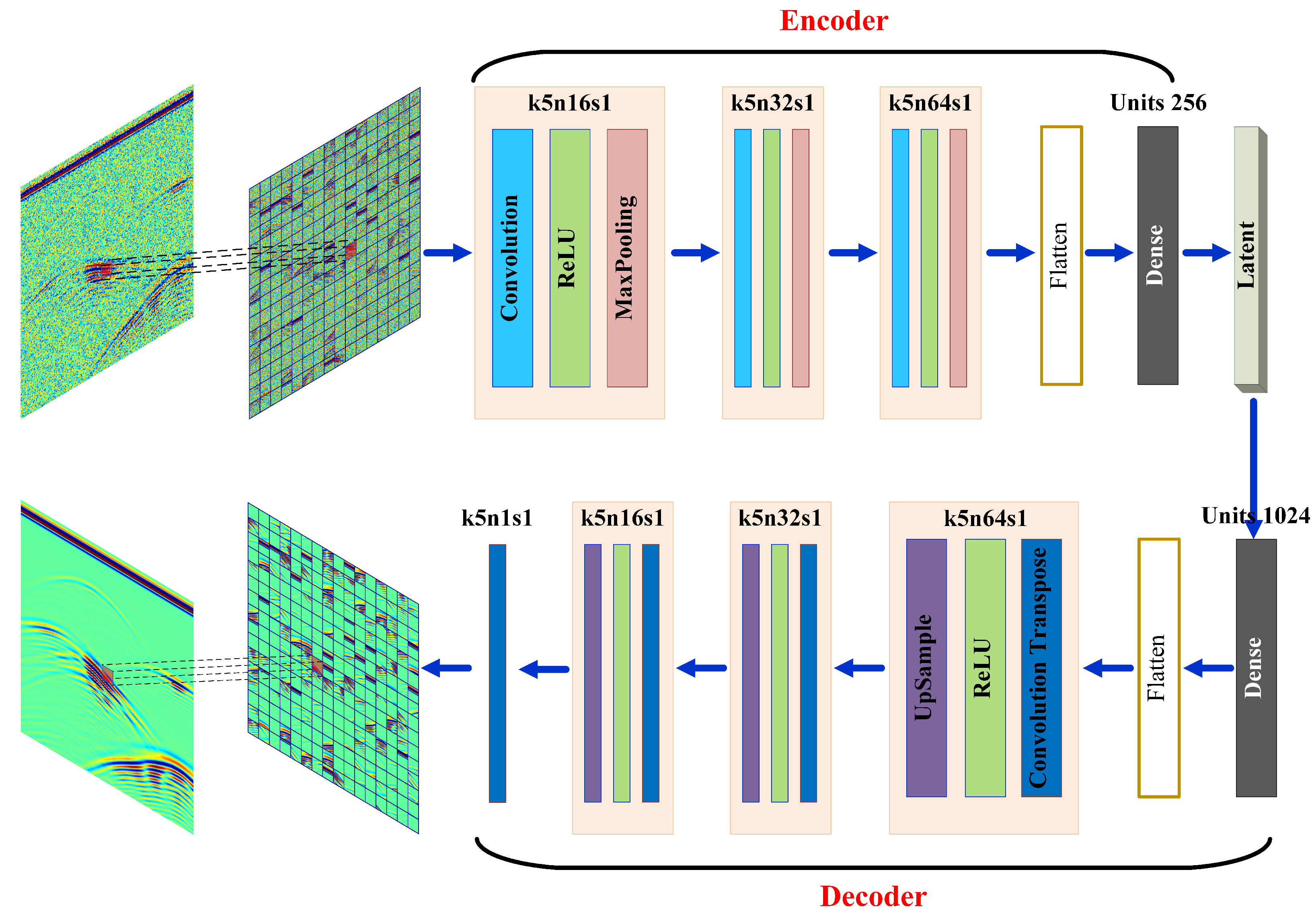
Figure 3 shows the network structure of a conventional CDAE. For the encoder part, the complete GPR profile data comprise considerable feature information; hence, if the entire profile dataset is used for the training data, more profile data will be required, which will overwhelm the available computational resources. Therefore, the profile data can be divided into several small blocks by sliding the window to convert the entire profile dataset into fragmented profile data by randomly arranging the slider data. The size of the slider is 32 × 32 and the sliding step is 4. In this way, each window slider contains less feature information. By adopting multiple complete sections of window slider information, the waveform feature information can be more effectively extracted without requiring excessive amounts of data, and heterogeneous images can be combined to boost the sample size for improved noise attenuation performance. Subsequently, fragmented profile data are selected in batches with a size of 64 and they are passed through three convolutional layers in succession. A connected max-pooling layer is encountered after each convolutional layer. The data from the last max-pooling layer are expanded in one dimension and then passed into the fully connected layer as the input data. Finally, a 1D latent vector is output to complete the learning process of the encoder with regard to the data features. The decoder part can be understood as the reverse operation of the encoder: its purpose is to restore the latent vector and ultimately obtain the profile with the same dimensions as the encoder input, thereby completing the denoising of the GPR data.
The above content elaborates on the detailed principle and essence of conventional CDAEs. During the implementation of conventional CDAEs, we found that these autoencoders may encounter problems, such as overfitting and the representational bottlenecks and vanishing gradients that are commonly found in deep learning. Therefore, it is necessary to modify the structure of conventional CDAEs to further improve their performance.
Algorithm 1 is the CDAE process. First, we segment the GPR datasets into patches x ˜ and segment the GPR data without noise into x in the same way.
Algorithm 1 The Training Process for CDAEs
Input:  x ˜ , x
Output:  C D A E s w i t h p a r a m e t e r W a n d b
1:
Initialization e p o c h = 0 , C D A E s w i t h p a r a m e t e r W a n d b
2:
while e p o c h < e p o c h s do
3:
     l a t e n t = Encoder.fit( x ˜ )
4:
     x ¯ = Decoder.fit( l a t e n t )
5:
     m s e = MSE( x , x ¯ )
6:
    Update W a n d b using backpropagation
7:
end while
8:
return C D A E s w i t h p a r a m e t e r W a n d b

3. Network Structure Modification Strategy

3.1. Overfitting Problem and Dropout Regularization Layer

The basic problem of machine learning is to strike a balance between optimization and generalization. By adjusting the hyperparameters, such as the weight value and bias of the model, to obtain better performance on the training data, we will make this process an optimization and use the adjusted model to predict any unknown data. Determining the process of model performance on unknown data is called generalization. Of course, the goal is to achieve good generalization, but generalization is uncontrollable: the only way is to adjust the model that is based on the training data.
At the beginning of the training, optimization and generalization tasks are associated: the loss of verification data gradually decreases with the loss of training data. At this stage, this model is said to be underfit and, thus, further development is necessary. The network, at this time, does not model all of the relevant patterns in the training data. However, after a certain period of epochs on the training data, the generalization task ceases to improve, and the validation metrics plateau and then begin to degrade; at the same time, the generalization loss no longer decreases, but instead begins to increase. In this case, the model is characterized by overfitting; that is, the model begins to learn patterns specific to the training data. The usual solution is to obtain more training data in order to prevent the model from learning irrelevant patterns or from memorizing the training data. However, the training data are limited by both the number of samples and the computer hardware. Therefore, it is necessary to optimize the model from other perspectives to avoid overfitting.
For the model that was learned by the neural network, when given some training data and network architecture, there will be many weights and biases to explain the data, which is, the network is nonunique. The principle of the dropout regularization layer is to randomly drop out (i.e., set to zero) a number of output features of the layer during training. The purpose of this operation is to introduce noise into the output values of a layer to interfere with the network, thereby disrupting happenstance nonsignificant patterns and reducing the overfitting of the model by eliminating the memorization of the neural network on the training datasets [35,36].

3.2. Local Receptive Field and Atrous Convolution

The local receptive field, which is an important concept in a convnet, is defined as the size of the input layer area that determines an element of the output result of a certain layer in a convnet. In mathematical language, the local receptive field is a mapping of an element of output in a certain layer to an input layer in a convnet.
Figure 4a depicts the 1-atrous convolution of size 3 × 3 , which is the same as the convolution operation. Likewise, Figure 4b illustrates the 2-atrous convolution of size 3 × 3 ; however, although the actual convolution kernel size is still 3 × 3 , since the atrous number is 2, the image block has a size of 7 × 7 , which indicates that the local receptive field is analogous to a 7 × 7 convolution kernel. In Figure 4, only the red dots have weights for the convolution operation, while the weights of the remaining points are all 0, so no operation is performed. From this figure, there are only nine weight values for the actual convolution operation, but the local receptive field of the convolution has increased to 7 × 7 . Therefore, for data that need additional features, atrous convolution can be used to obtain a larger local receptive field and reduce the memory consumption of the computer.

3.3. Loss of Detailed Information and Residual Connections

First, in the conventional sequential model, each successive presentation layer is built on top of the previous layer, which means that the model can only access the information that is contained in the activation of the previous layer. If the features of one layer have too few dimensions, then the model will be constrained by how much information the activations of this layer can contain. Generally, each output will be a previous operation as an input; accordingly, if one operation results in the loss of information, all of the downstream operations will fail to recover the lost information. In other words, any loss of information is permanent. This concept is considered to be representational bottleneck in deep learning.
Second, gradient backpropagation is the main algorithm used to train deep neural networks. Its working principle is to backpropagate the feedback gradient signal from the output layer to the shallower layer. If this feedback signal must propagate through the deep stack, then the signal may be attenuated or even lost entirely, which makes the network training almost unchanged or impossible to train. This problem is called the vanishing gradient problem.
To solve these two problems, the residual-connection structure was proposed. The residual connection involves making the output of the shallower layer available as the input of the deeper layer, effectively creating a shortcut in the sequential network. However, instead of simply linking it to the subsequent activation, the previous output is added to the subsequent activation. Because any loss of information is permanent, the earlier information is reinjected downstream, and residual connections may partially avoid representational bottlenecks for deep learning models. In addition, the introduction of the path’s remaining connections may transmit information in parallel to a purely linear main layer stack, thereby facilitating the deep layers of the stack by any propagation gradient [37,38].
For the denoising attenuation problem of GPR data, the loss of information only occurs during the process of transforming profile data into feature latent vectors. Therefore, the sliding block part can be omitted, and only the autoencoder structure needs to be modified. Figure 5 shows the modified autoencoder structure.

4. Selection of Model Parameters and Model Testing

4.1. Training Dataset and Validation Dataset

We randomly generated 200 sets of GPR profiles, including 100 stochastic irregular underground anomaly models and 100 stochastic tunnel lining anomaly models, in order to train a CDAE model. The number, shape, size, location, and physical parameters (such as permittivity and conductivity) of the anomalies in the two model sets are all completely randomly generated. By adding Gaussian noise of different levels to the GPR anomaly profiles and using the sliding window method, each GPR profile is divided into multiple image blocks to obtain more detailed waveform features. In addition, because the GPR profile data contain considerable amounts of redundant information, using each entire profile for the training dataset would introduce substantial redundancy. The sliding window method can avoid this phenomenon and obtain more training data with fewer profiles to meet the training requirements of a neural network by combining heterogeneous images to boost the sample size for improved noise attenuation performance. Figure 6 depicts rhe specific dataset establishment process. When using this method to construct a dataset, in order to avoid the possibility that the window signal loses the original signal information when the data are divided into window blocks, which are mainly hyperbolas spanning the entire “bigger” original image, we need to select the window size flexibly according to the frequency of the signal. The size of the sliding window block in this paper is 32 × 32 and the sliding step is 4. By preprocessing 200 sets of GPR profiles with noise and randomly arranging sliding window blocks, we obtained 649,800 samples of data as the input for the autoencoder. We employ the mini-batch stochastic gradient descent method, together with the Adam optimizer, to minimize the above loss.
In order to test the generalization ability of the model, the 649,800 samples were divided into three parts: 2000 datasets were randomly selected as the validation dataset to participate in the validation and evaluation during the iterative model training; 2000 datasets were randomly selected as evaluation data to verify and evaluate the final model result; and, the remaining datasets were used as training datasets to iteratively train the model. We use synthetic data to train the network model and apply the network to unknown data (synthetic data or measured data).

4.2. Structure of the Model

CDAEs consist of both encoders and decoders, and Table 2 describes their hierarchical structure. In the encoder part, we input GPR profile datasets with dimensions of 32 × 32 × 1 , and we obtain a 1D latent vector with a length of 256 after training. Subsequently, the GPR profile features are transformed into a set of low-dimensional latent vectors, where Conv2D represents the 2D convolutional layer in Table 2; the input receives a 4D tensor; and, the output shape of each layer represents the total number of samples, the image size and the image depth. In the decoder part, the input receives a 1D latent vector with a length of 256, and then GPR profile datasets with dimensions of 32 × 32 × 1 are finally obtained after training. At this point, the reconstruction of the low-dimensional latent vector is complete, where Conv2DTr represents the 2D deconvolution layer; the input receives a 1D vector; and, the output shape of each layer represents the total number of samples, the image size and the image depth.
Connecting the encoder and the decoder end to end, the output of the encoder is used as the input of the decoder, as shown in Figure 3. The GPR profile data are first converted into a low-dimensional latent vector by the encoder, and then the low-dimensional latent vector is finally reconstructed into GPR profile data by the decoder. So far, the construction of the CDAE network structure has been completed.

4.3. Selection of Parameters

Table 2 demonstrates that the number of filters used by the convolutional layers are 16, 32 = m and 64; the length of the 1D latent vector is 256; the convolution kernel size is 5 × 5 ; and, the number of training epochs is set to 10. After repeatedly testing the model performance and the above parameters, the recommended parameters for the best optimization are given in Table 3. In this table, the “Loss” represents the training loss during the training process, and the “Validation Loss” represents the loss obtained by using the data that are not involved in the training process to verify the network performance.
Analyzing the parameters presented in Table 3 demonstrates that for a GPR profile with noise, due to its low feature dimension, when selecting a larger filter depth, there will be significant performance degradation, and a larger local receptive field will be required; when the latent vector is excessively large, redundant data will be encountered. Therefore, the feature dimension of the GPR profile determines the optimal parameters of CDAEs.

5. Strategy of Modifying the Network Structure

5.1. Adding the Dropout Regularization Layer

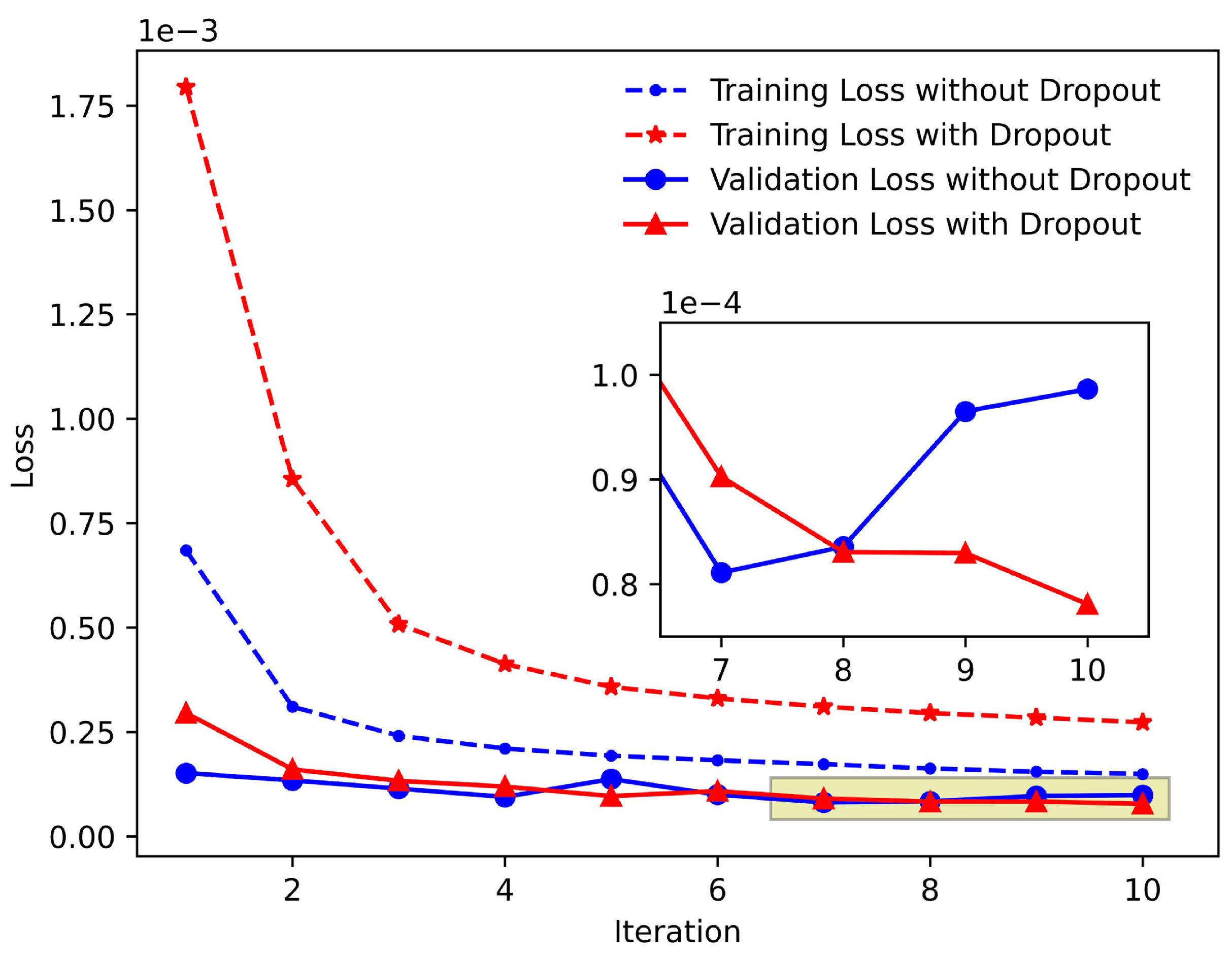
In order to reduce the overfitting problem caused by the neural network memorizing the training data, a dropout regularization layer is added after each convolutional layer and deconvolution layer of CDAEs, and some output features of this layer are randomly dropped out to disrupt happenstance nonsignificant patterns and reduce the overfitting of the model by removing the training data memorized by the neural network, as shown in Figure 5. Figure 7 presents a comparison of the training loss and verification loss after 10 epochs of CDAEs. The blue line represents the loss of CDAEs; and, the red line represents the loss of the dropout CDAEs (D-CDAEs). In this paper, the dropout ratio is set to 0.2 , which means that the output values of this layer are excluded at a ratio of 0.2 .
Figure 7 indicates that the training loss of CDAEs is smaller than that of D-CDAEs, which is due to the characteristics of the dropout regularization layer. Each time the data pass through the dropout regularization layer, the data will be dropped out according to the established ratio, which is equivalent to introducing noise and it has a certain impact on the training loss. From the overall trend, the training losses of CDAEs and D-CDAEs present decreasing trends. In addition, D-CDAEs have a smaller and more stable validation loss when compared with CDAEs. To more accurately distinguish the details of the two curves, we partially enlarge the curves in Figure 7. The validation loss of CDAEs reached its minimum value at the seventh training epoch and then began to increase, suggesting that the model started to overfit at this time. The verification loss of D-CDAEs decreased gradually during the iterative training without overfitting. Therefore, the addition of the dropout regularization layer can increase the training loss to a certain extent while avoiding the overfitting phenomenon.

5.2. Replacing Convolution with Atrous Convolution

A tunnel lining model containing an “H-beam” was established to illustrate the influence of using atrous convolution instead of convolution on the attenuation of noise [39], as shown in Figure 8. The dimensions of the model are 5.0 m × 2.5 m. From top to bottom, the model consists of steel, a waterproof board, and an H-beam. The window length of the profile is 70 ns, and the antenna excites a Ricker wavelet with a frequency of 400 MHz. The finite difference time-domain (FDTD) algorithm is used for forward modeling [40].
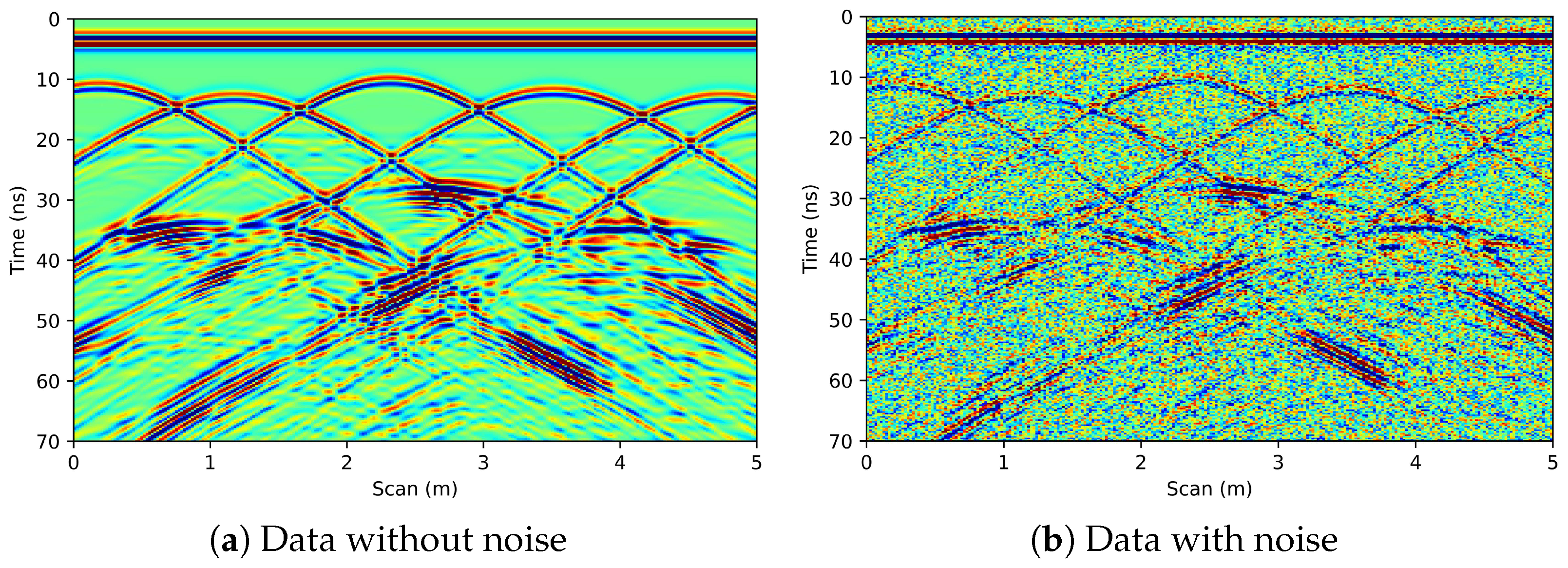
Figure 9a depicts the GPR forward profile (raw data without noise). Multiple strong reflection hyperbolas from the steel are detected at the top. The interface of the waterproof board is also clearly discernible, but the reflected wave energy is relatively weak. A strong reflection from the H-beam can be seen at 30–40 ns. In addition, a significant number of multiples (i.e., waves that are reflected multiple times) are observed due to the interactions of the anomalies with electromagnetic waves, which complicates the profile information greatly. Random Gaussian noise was added to the GPR profile to form a noisy profile, as shown in Figure 9b (data contaminated by noise). Because the existence of noise seriously affects the quality of the profile data, the multiples and the weak reflections from the waterproof board are completely submerged by the noise, and the strong reflections from the anomalies are also damaged. To compare the noise level that is introduced by these methods more intuitively, we introduce the SNR shown in (7) as the evaluation criterion:
S N R = 10 log 10 x = 1 N x y = 1 N y ( f ( x , y ) ) 2 x = 1 N x y = 1 N y ( f ( x , y ) f ^ ( x , y ) ) 2
Among them, N x and N y represent the size of the data (that is, the data is N x t i m e s N y ); f ( x , y ) represents the original data; and f ^ ( x , y ) represents the data with noise. From a statistical perspective, in regard to the difference between the original data and the evaluation data, the smaller the noise level, the greater the effective SNR. Therefore, a larger SNR value indicates better noise attenuation performance.
Each GPR profile has large amounts of redundant data and, hence, a larger local receptive field is necessary to obtain more feature information. Therefore, we proposed using atrous convolution to replace convolution. CDAEs and AD-CDAEs were used to denoise the profile in Figure 9b, and the noise attenuation results are shown in Figure 10a,b, respectively; the residuals after noise attenuation are shown in Figure 11a,b, respectively.
Analyzing both Figure 10b, Figure 11a,b and Figure 12c reveals that the two models can effectively attenuate the noise on the GPR profile; in particular, the reflected waves from the waterproof board and the multiples are all reconstructed. However, CDAEs also destroy the information of the original profile while removing the noise, and the damage to the waveforms is somewhat obvious. In contrast, as shown in the residual profile, AD-CDAEs retain more waveform information than CDAEs and maintain higher fidelity with respect to the effective feature information of the radar wavefield.

5.3. Modifying the Network Structure by Residual Connections

Because deep learning suffers from the problems of representational bottlenecks and vanishing gradients, CDAEs are prone to destroying useful feature information while removing Gaussian noise; this tendency causes a large amount of data to be lost and, thus, CDAEs do not meet the noise attenuation requirements of GPR profiles. We used residual connections to further modify the structure of the network and obtained the modified atrous-dropout-CDAEs-residual network (AD-CDAEs-ResNet) that is presented in Figure 5, which is the final version of CDAEsNSO. The second convolutional layer is no longer limited to receiving the output from only the first convolutional layer, but it can also receive the original profile data, which carry the most authentic information. Introducing a path to transport purely linear information helps to propagate gradients through arbitrarily deep stacks of layers, effectively preventing the loss of information and the problem of vanishing gradients. To verify the noise attenuation effect of the modified network structure on the GPR profile, we again took the H-beam model (Figure 8) as an example. Figure 12c and Figure 13c show the noise attenuation result and the residual of AD-CDAE-ResNet, respectively.
These results show that the reflected waves from the waterproof board and the multiples are well preserved, and that the information in the original profile can be retained with high fidelity, indicating that AD-CDAEs-ResNet can effectively remove random noise and resolve the problems of representational bottlenecks and vanishing gradients. To more intuitively compare the noise attenuation effects of several autoencoders, the SNR is calculated before and after the attenuation of noise, and Table 4 shows the results.
Comparing the SNRs presented in Table 4 exposes that CDAEs have the worst noise attenuation effect among the three methods due to the substantial removal of effective information. AD-CDAEs can partly improve the noise attenuation effect by increasing the size of the local receptive field. Ultimately, the AD-CDAEs-ResNet achieves the best noise attenuation effect, because it solves the problems of representational bottlenecks and vanishing gradients.

5.4. Comparison with Other Typical Noise Attenuation Methods

We selected several commonly used noise attenuation algorithms to highlight that CDAEs can better distinguish between noise data and effective signals and have a better effect on noise attenuation. Because AD-CDAEs-ResNet is not based on a fixed-base transformation method, it can be autonomous. The self-adjustment is carried out according to the characteristics of various signals, so the signal has less damage, whereas the method of using a fixed-base transformation means more damage to the signal. Based on this principle, we chose the commonly used method based on fixed-base transformation. In addition, we also selected a signal-based SR strategy to process the data. Similarly, the sparse representation strategy cannot be self-adjusted according to the characteristics of various signals. For this reason, we selected the wavelet transform method and K-singular value decomposition (K-SVD) method according to these methods in Table 1 to process the profile data in Figure 8. Figure 12 shows the noise attenuation result, and Figure 13 shows the noise residual. Table 5 shows the detailed SNR data.
The results shown in Figure 12 and Figure 13 indicate that, by comparing the noise attenuation results and noise residuals of AD-CDAEs-ResNet and other methods, the wavelet transform method that is based on a fixed basis destroys the effective signal, although it has a certain degree of noise suppression. Because the K-SVD method is based on a dictionary learning strategy, a better overcomplete dictionary is obtained through dictionary learning, so a better noise attenuation effect is obtained, and the damage to the signal is also correspondingly reduced. However, from the point of view of the noise residual, this method is still more serious to the effective signal, especially the position with strong signal energy (direct wave and strong reflection area), and it even causes a distortion of the direct wave signal. Finally, the AD-CDAEs-ResNet algorithm that is proposed in this paper obtains the optimal effect, and it can effectively distinguish the noise signal from the effective signal, and it perfectly suppresses the noise without causing a distortion of other signals. In addition, from the comparison of the SNR values presented in Table 5, the same conclusion can be obtained.
We list the SNRs of these algorithms in the form of a histogram to summarize the abovementioned noise attenuation algorithms and compare the improvement of SNRs by various algorithms, as shown in Figure 14. The histogram conveniently provides a comparison and description.

6. Results

6.1. Synthetic Data

To illustrate the adaptability of AD-CDAEs-ResNet to complex models, Gaussian random noise and Gaussian spike impulse noise, we designed the tunnel lining model that is shown in Figure 15 with the dimensions of 5.0 m × 2.5 m. From top to bottom, there are two linings with a relative permittivity of 9, an uncompacted part filled with water, and cavities. The window length of the profile is 70 ns, and the antenna excites a Ricker wavelet with a frequency of 400 MHz. The FDTD algorithm is used for forward modeling.
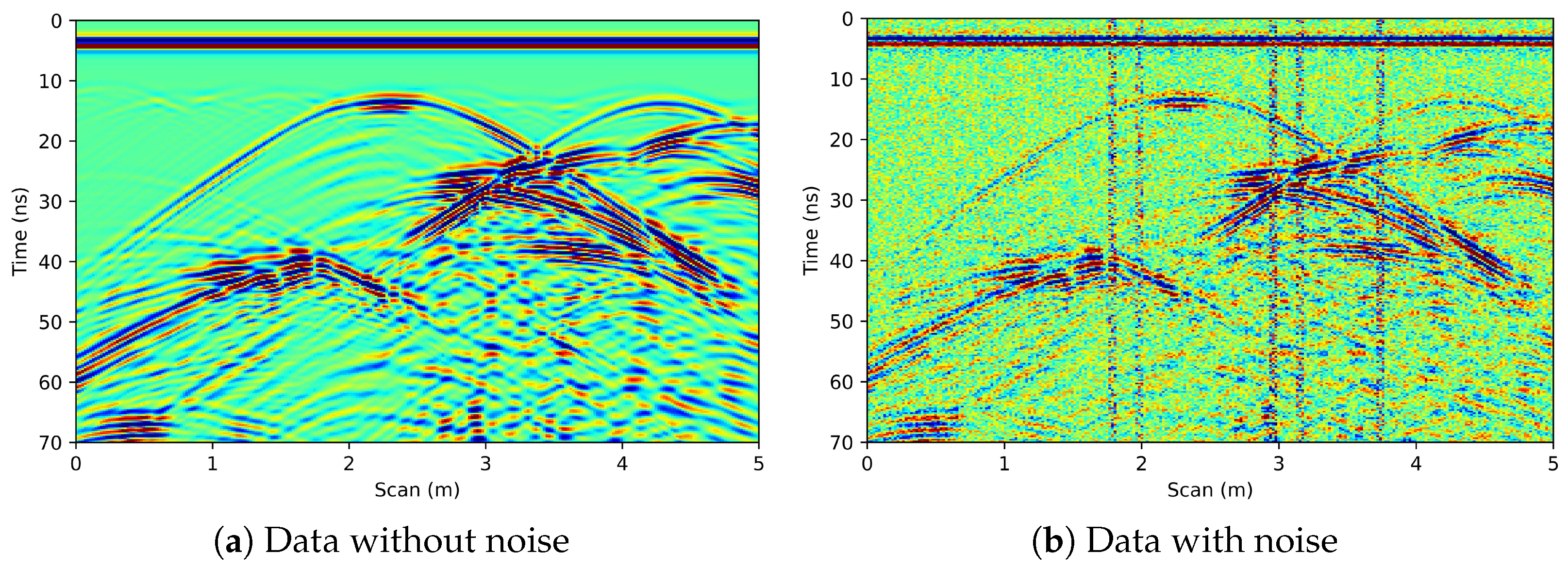
Figure 16a presents the GPR forward profile. We can identify the reflected waves, diffracted waves, and multiples generated by the interfaces between the surrounding rock and the two linings, the water-bearing fractures, and the water-free fractures. The positions, sizes, and shapes of the geological anomalies can be roughly estimated by analyzing the shapes of the radar reflections. Gaussian random noise and high-interference Gaussian spike impulse noise were added to the profile to obtain the noisy GPR profile that is shown in Figure 16b. Because of the influence of this Gaussian noise, the waves reflected from the second lining are submerged by noise, and there are 5 instances in which vertical Gaussian impulse spikes disturb the data section; these phenomena seriously affect the interpretation of the data.

6.2. Field Data

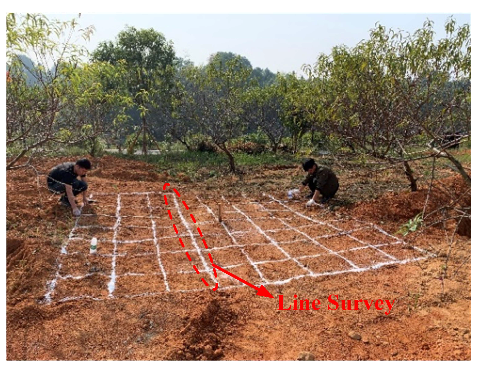
We selected a pipeline field dataset to validate the effectiveness of AD-CDAEs-ResNet to illustrate the practicality of the proposed algorithm. The data were collected using the SIR-4000 GPR with an antenna that excites a wavelet with a frequency of 400 MHz as the excitation signal. The data were collected from Huangxiu Agricultural Culture Park, Yueyang city, Hunan Province. We used the spot measurement mode with a spot distance of 0.05 m for the measurement. A total of 111 channels of data were collected, and the recording time was 60 ns. Figure 17 shows the radar survey lines and field measurements.

7. Discussion

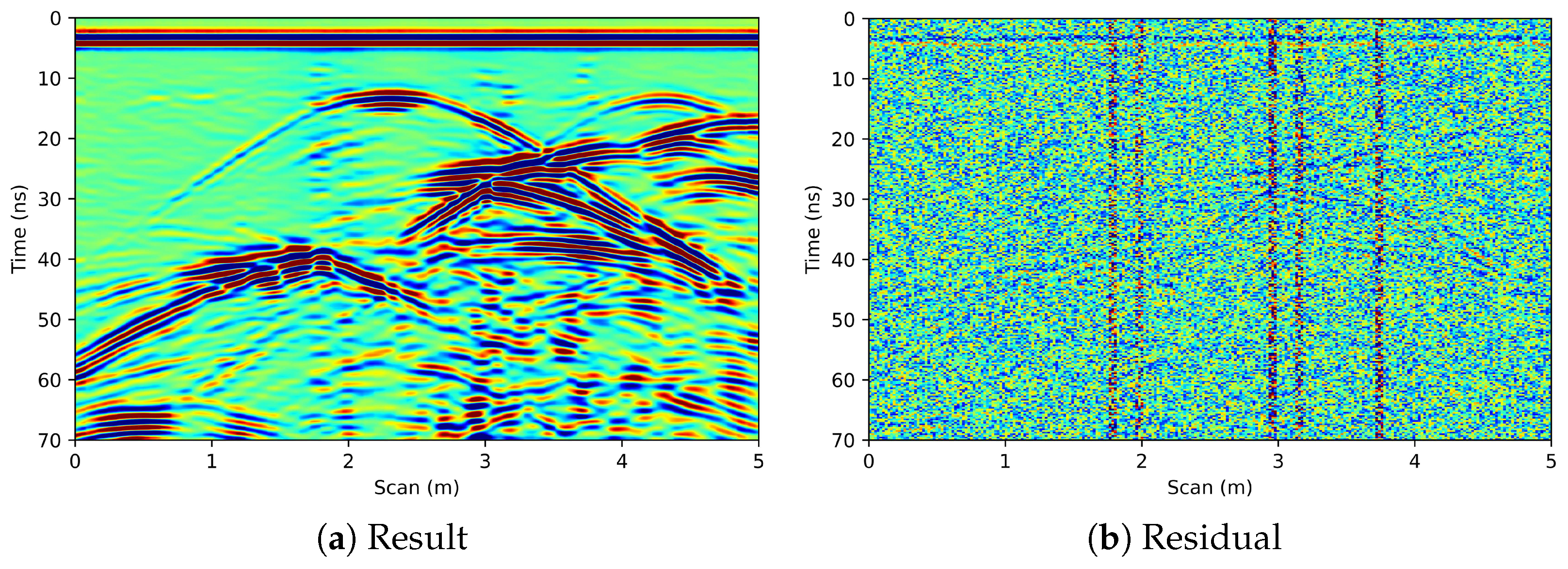
Figure 18a shows the noise attenuation result that was obtained by applying AD-CDAEs-ResNet to the mixed noise profile containing both Gaussian spike impulse noise and Gaussian noise. This figure indicates that AD-CDAEs-ResNet can effectively remove mixed noise while reliably preserving information of the reflected waves and multiples. Figure 18b presents the residual of AD-CDAEs-ResNet, indicating that the proposed algorithm does less damage to the information in the original profile and maintains better fidelity. The SNRs before and after the attenuation of noise are 9.7392 dB and 27.1753 dB, respectively, verifying the effectiveness of the algorithm.
Figure 19a shows a section of the GPR data that were acquired in the field. Two groups of Gaussian spike impulse noise are circled, and the reflected waves from the pipelines are not particularly clear. Figure 19b presents the noise attenuation result of AD-CDAEs-ResNet. Hyperbolic diffracted waves from the upper and lower interfaces of pipelines are readily detectable, and the layer interfaces at approximately 56 ns can also be identified. Figure 19c illustrates the residual of AD-CDAEs-ResNet, containing almost all noise and very little information pertaining to reflected waves. From these residuals, it is evident that the three groups of Gaussian spike impulse noise are obviously removed, which confirms that the proposed noise attenuation algorithm does less damage to the information in the original profile and achieves an improved noise attenuation effect.

8. Conclusions

When compared with data domain transformation-based methods and SR-based techniques, convolutional denoising autoencoders (CDAEs) that are based on deep learning can adjust themselves according to the features of signals. CDAEs represent a kind of unsupervised learning neural network that can adapt to the denoising algorithm. However, when CDAEs are directly applied to attenuate the noise of GPR data, they encounter various problems, including overfitting, the size of the local receptive field, and the representation bottlenecks and vanishing gradients that are typical of deep learning. Therefore, the authors proposed some network structure optimization strategies, such as the addition of a dropout regularization layer, an atrous convolution layer and a residual-connection structure, and obtained a new GPR noise attenuation algorithm, namely CDAEsNSO.
CDAEsNSO, which was proposed based on CDAEs, can effectively remove random noise and Gaussian spike impulse noise from GPR data. Moreover, the proposed algorithm does little damage to useful waveforms, such as information of reflected waves, diffracted waves, and multiples, in the original profile and maintains high data fidelity, effectively improving the noise attenuation effect. At the same time, this method also has certain limitations. For example, a large amount of data is required as learning samples during network training, and the network is a computationally intensive operation during the training process, which requires a higher level of computer equipment. In terms of network training, it is also more time consuming than other algorithms. However, once the network training is completed, the model can be used directly to achieve end-to-end processing operations. In the final processing stage, when compared with other algorithms, it does not need to be recalculated.
Therefore, the efficiency of data processing is higher.
The GPR profiles contain considerable amounts of redundant information. Nevertheless, the detailed features in a whole profile are sparse. Therefore, we proposed the sliding window method to process GPR profile data to obtain training datasets by combining heterogeneous images to boost the sample size for improved noise attenuation performance. This method not only avoids the redundancy of information while obtaining more detailed waveform characteristics, but also utilizes fewer GPR data to obtain more training datasets that meet the training requirements of CDAEs.

Author Contributions

Conceptualization, D.F., X.W. (Xiangyu Wang) and X.W. (Xun Wang); methodology, X.W. (Xun Wang); validation, X.W. (Xiangyu Wang) and X.W. (Xun Wang); formal analysis, X.W. (Xiangyu Wang); resources, S.D. and H.Z.; writing—original draft preparation, X.W. (Xiangyu Wang); writing—review and editing, X.W. (Xiangyu Wang), X.W. (Xun Wang) and H.Z.; visualization, X.W. (Xiangyu Wang); supervision, D.F. and X.W. (Xun Wang); project administration, D.F.; funding acquisition, D.F. All authors have read and agreed to the published version of the manuscript.

Funding

This research was funded by the National Natural Science Foundation of China under grant numbers 42074161 and 41774132. The APC was funded by the Free Exploration Project of Central South University under Grant 2020zzts185.

Institutional Review Board Statement

Not applicable.

Informed Consent Statement

Not applicable.

Data Availability Statement

The code uses Python 3.8 + TensorFlow 2.0 version and is based on the MIT license. The Python code used to reproduce the results and all the physical models and GPR profile data in this article can be publicly accessed through https://github.com/nephilim2016/AutoEncoder-for-GPR-Denoise.

Acknowledgments

The authors would like to thank Yi Lei, the School of Geosciences and Info-Physics, Central South University, and the Key Laboratory of Metallogenic Prediction of Nonferrous Metals for giving us the opportunity to collect the field data. They would also like to thank the support of TensorFlow and Keras for this research. In addition, they would also like to thank American Journal Experts (AJE) and Cory R. for editing this article.

Conflicts of Interest

The authors declare no conflict of interest.

Abbreviations

The following abbreviations are used in this manuscript:
GPRground penetrating radar
SNRsignal-noise ratio
CDAEsconvolutional denoising autoencoders
CDAEsNSOconvolutional denoising autoencoders with network structure optimization
AD-CDAEsatrous-dropout convolutional denoising autoencoders
ResCDAEsresidual-connection convolutional denoising autoencoders
ReLUrectified linear unit
K-SVDK-singular value decomposition

References

  1. Dong, Z.; Ye, S.; Gao, Y.; Fang, G.; Zhang, X.; Xue, Z.; Zhang, T. Rapid detection methods for asphalt pavement thicknesses and defects by a vehicle-mounted ground penetrating radar (GPR) system. Sensors 2016, 16, 2067. [Google Scholar] [CrossRef] [Green Version]
  2. Khamzin, A.K.; Varnavina, A.V.; Torgashov, E.V. Utilization of air-launched ground penetrating radar (GPR) for pavement condition assessment. Constr. Build. Mater. 2017, 141, 130–139. [Google Scholar] [CrossRef]
  3. Diamanti, N.; Annan, A.P.; Redman, J.D. Concrete bridge deck deterioration assessment using ground penetrating radar (GPR). J. Environ. Eng. Geophys. 2017, 22, 121–132. [Google Scholar] [CrossRef]
  4. Solla, M.; Lagüela, S.; Fernández, N. Assessing rebar corrosion through the combination of nondestructive GPR and IRT methodologies. Remote Sens. 2019, 11, 1705. [Google Scholar] [CrossRef] [Green Version]
  5. Rasol, M.A.; Pérez-Gracia, V.; Fernandes, F.M.; Pais, J.C.; Santos-Assunçao, S.; Santos, C.; Sossa, V. GPR laboratory tests and numerical models to characterize cracks in cement concrete specimens, exemplifying damage in rigid pavement. Measurement 2020, 158, 107662. [Google Scholar] [CrossRef]
  6. Liu, X.; Dong, X.; Xue, Q. Ground penetrating radar (GPR) detects fine roots of agricultural crops in the field. Plant Soil. 2018, 423, 517–531. [Google Scholar] [CrossRef]
  7. Lai, W.; Chang, R.K.; Sham, J.F. Blind test of nondestructive underground void detection by ground penetrating radar (GPR). J. Appl. Geophys. 2018, 149, 10–17. [Google Scholar] [CrossRef]
  8. Terrasse, G.; Nicolas, J.M.; Trouvé, E. Application of the Curvelet Transform for clutter and noise removal in GPR data. IEEE J. Sel. Top. Appl. Earth Observ. Remote Sens. 2017, 10, 4280–4294. [Google Scholar] [CrossRef]
  9. He, T.; Shang, H. Direct-wave denoising of low-frequency ground-penetrating radar in open pits based on empirical curvelet transform. Near Surf. Geophys. 2020, 18, 295–305. [Google Scholar] [CrossRef]
  10. Gan, L.; Zhou, L.; Liu, S.M. A de-noising method for GPR signal based on EEMD. Appl. Mech. Mater. Trans. Tech. Publ. Ltd. 2014, 687, 3909–3913. [Google Scholar] [CrossRef]
  11. Li, J.; Liu, C.; Zeng, Z.F.; Chen, L.N. GPR Signal Denoising and Target Extraction with the CEEMD Method. IEEE Geosci. Remote Sens. Lett. 2015, 12, 1615–1619. [Google Scholar]
  12. Ostoori, R.; Goudarzi, A.; Oskooi, B. GPR random noise reduction using BPD and EMD. J. Geophys. Eng. 2018, 15, 347–353. [Google Scholar] [CrossRef]
  13. Zhang, X.; Feng, X.; Zhang, X. Dip Filter and Random Noise Suppression for GPR B-Scan Data Based on a Hybrid Method in f-x Domain. Remote Sens. 2019, 11, 2180. [Google Scholar] [CrossRef] [Green Version]
  14. Kobayashi, M.; Nakano, K. A denoising method for detecting reflected waves from buried objects by ground-penetrating radar. Electr. Commun. Jpn. 2013, 96, 1–13. [Google Scholar] [CrossRef]
  15. Huang, W.L.; Wu, R.S.; Wang, R. Damped dreamlet representation for exploration seismic data interpolation and denoising. IEEE Trans. Geosci. Remote Sens. 2018, 56, 3159–3172. [Google Scholar] [CrossRef]
  16. Qiao, X.; Fang, F.; Zhang, J. Ground Penetrating Radar Weak Signals Denoising via Semi-soft Threshold Empirical Wavelet Transform. Ingénierie Syst. Inf. 2019, 24, 207–213. [Google Scholar] [CrossRef]
  17. Chen, L.; Zeng, Z.; Li, J. Research on weak signal extraction and noise removal for GPR data based on principal component analysis. Glob. Geol. 2015, 18, 196–202. [Google Scholar]
  18. Huang, W.; Wang, R.; Chen, X. Damped sparse representation for seismic random noise attenuation. In SEG Technical Program Expanded Abstracts 2017; Society of Exploration Geophysicists: Tulsa, OK, USA, 2017; pp. 5079–5084. [Google Scholar]
  19. Deng, L.; Yuan, S.; Wang, S. Sparse Bayesian learning-based seismic denoise by using physical wavelet as basis functions. IEEE Geosci. Remote Sens. Lett. 2017, 14, 1993–1997. [Google Scholar] [CrossRef]
  20. Bi, W.; Zhao, Y.; An, C. Clutter elimination and random-noise denoising of GPR signals using an SVD method based on the Hankel matrix in the local frequency domain. Sensors 2018, 18, 3422. [Google Scholar] [CrossRef] [Green Version]
  21. Liu, L.; Ma, J. Structured graph dictionary learning and application on the seismic denoising. IEEE Trans. Geosci. Remote Sens. 2018, 57, 1883–1893. [Google Scholar] [CrossRef]
  22. Bai, X.; Peng, X. Radar image series denoising of space targets based on Gaussian process regression. IEEE Trans. Geosci. Remote Sens. 2019, 57, 4659–4669. [Google Scholar] [CrossRef]
  23. Zhang, J.; Zhang, H.; Li, Y. A Morphological component analysis based on mixed dictionary for signal denoising of ground penetrating radar. Int. J. Simul. Process. Model. 2019, 14, 431–441. [Google Scholar] [CrossRef]
  24. Li, H.; Wang, R.; Cao, S. Mathematical morphological filtering for linear noise attenuation of seismic data. Geophysics 2016, 81, V159–V167. [Google Scholar] [CrossRef]
  25. Huang, W.; Wang, R.; Zhang, D. A method for low-frequency noise suppression based on mathematical morphology in microseismic monitoring. Geophysics 2017, 82, V369–V384. [Google Scholar] [CrossRef]
  26. Li, J.; Le Bastard, C.; Wang, Y.; Gang, W.; Ma, B.; Sun, M. Enhanced GPR Signal for Layered Media Time-Delay Estimation in Low-SNR Scenario. IEEE Geosci. Remote Sens. Lett. 2016, 13, 299–303. [Google Scholar] [CrossRef]
  27. Gondara, L. Medical image denoising using convolutional denoising autoencoders. In Proceedings of the 2016 IEEE 16th International Conference on Data Mining Workshops (ICDMW), Barcelona, Spain, 12–15 December 2016; pp. 241–246. [Google Scholar]
  28. Zhou, H.; Feng, X.; Dong, Z.; Liu, C.; Liang, W. Application of Denoising CNN for Noise Suppression and Weak Signal Extraction of Lunar Penetrating Radar Data. Remote Sens. 2021, 13, 779. [Google Scholar] [CrossRef]
  29. Grais, E.M.; Plumbley, M.D. Single channel audio source separation using convolutional denoising autoencoders. In Proceedings of the 2017 IEEE global conference on signal and information processing (GlobalSIP), Montreal, QC, Canada, 14–16 November 2017; pp. 1265–1269. [Google Scholar]
  30. Meng, Z.; Zhan, X.; Li, J. An enhancement denoising autoencoder for rolling bearing fault diagnosis. Measurement 2018, 130, 448–454. [Google Scholar] [CrossRef] [Green Version]
  31. Ashfahani, A.; Pratama, M.; Lughofer, E. DEVDAN: Deep evolving denoising autoencoder. Neurocomputing 2020, 390, 297–314. [Google Scholar] [CrossRef] [Green Version]
  32. Zhu, W.; Mousavi, S.M.; Beroza, G.C. Seismic signal denoising and decomposition using deep neural networks. IEEE Trans. Geosci. Remote Sens. 2019, 57, 9476–9488. [Google Scholar] [CrossRef] [Green Version]
  33. Saad, O.M.; Chen, Y. Deep denoising autoencoder for seismic random noise attenuation. Geophysics 2020, 85, V367–V376. [Google Scholar] [CrossRef]
  34. Kingma, D.P.; Ba, J. Adam: A method for stochastic optimization. arXiv 2014, arXiv:1412.6980. [Google Scholar]
  35. Dahl, G.E.; Sainath, T.N.; Hinton, G.E. Improving deep neural networks for LVCSR using rectified linear units and dropout. In Proceedings of the 2013 IEEE International Conference on Acoustics, Speech and Signal Processing, Vancouver, BC, Canada, 26–30 May 2013; pp. 8609–9613. [Google Scholar]
  36. Srivastava, N.; Hinton, G.; Krizhevsky, A. Dropout: A simple way to prevent neural networks from overfitting. J. Mach. Learn. Res. 2014, 15, 1929–1958. [Google Scholar]
  37. He, K.; Zhang, X.; Ren, S. Deep residual learning for image recognition. In Proceedings of the IEEE Conference on Computer Vision and Pattern Recognition, Las Vegas, NV, USA, 27–30 June 2016; pp. 770–778. [Google Scholar]
  38. Wu, S.; Zhong, S.; Liu, Y. Deep residual learning for image steganalysis. Multimed. Tools Appl. 2018, 77, 10437–10453. [Google Scholar] [CrossRef]
  39. Lyu, Y.; Wang, H.; Gong, J. GPR Detection of Tunnel Lining Cavities and Reverse-time Migration Imaging. Appl. Geophys. 2020, 17, 1–7. [Google Scholar] [CrossRef]
  40. Zhang, B.; Dai, Q.; Yin, X. A new approach of rotated staggered grid FD method with unsplit convolutional PML for GPR. IEEE J. Sel. Top. Appl. Earth Obs. Remote Sens. 2015, 9, 52–59. [Google Scholar] [CrossRef]
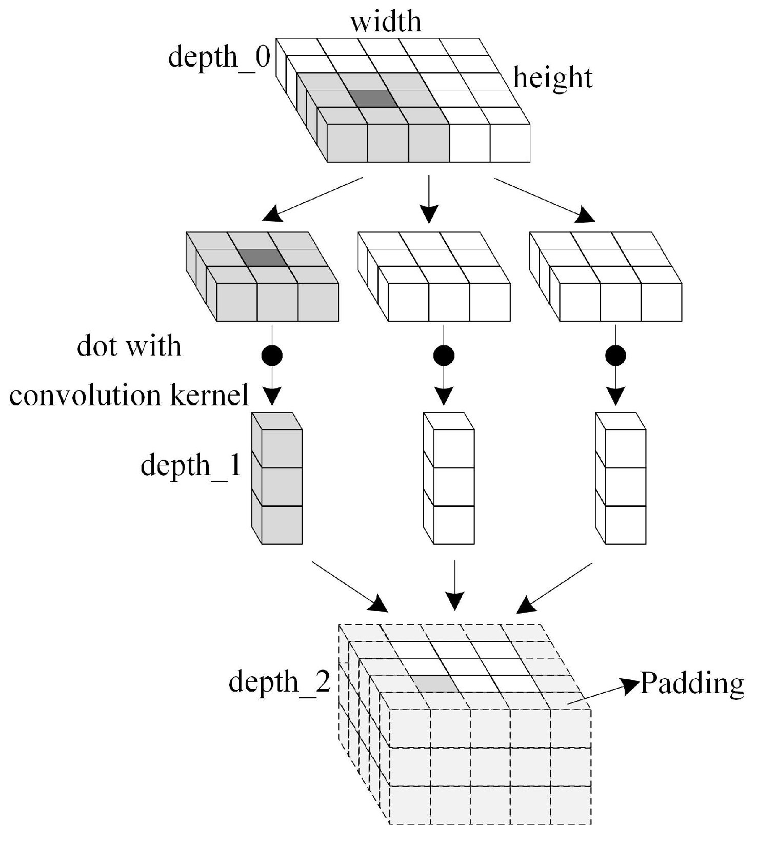
Figure 1. Representation of convolution.
Remotesensing 13 01761 g001
Figure 2. Feature maps of each layer.
Remotesensing 13 01761 g002
Figure 3. Structure of CDAEs.
Remotesensing 13 01761 g003
Figure 4. Atrous convolution.
Remotesensing 13 01761 g004
Figure 5. Structure of CDAEsNSO.
Remotesensing 13 01761 g005
Figure 6. Sliding window process.
Remotesensing 13 01761 g006
Figure 7. Loss function values of CDAEs and D-CDAEs.
Remotesensing 13 01761 g007
Figure 8. Tunnel lining model.
Remotesensing 13 01761 g008
Figure 9. Synthetic profile data of the tunnel lining.
Remotesensing 13 01761 g009
Figure 10. Noise attenuation result for the GPR profile of the tunnel lining.
Remotesensing 13 01761 g010
Figure 11. Noise attenuation residual for the GPR profile of the tunnel lining.
Remotesensing 13 01761 g011
Figure 12. Noise attenuation result for the GPR profile of the tunnel lining compared with other methods.
Remotesensing 13 01761 g012
Figure 13. Noise attenuation residual for the GPR profile of the tunnel lining compared with other methods.
Remotesensing 13 01761 g013
Figure 14. SNR histogram of various methods.
Remotesensing 13 01761 g014
Figure 15. The model of the complex tunnel lining.
Remotesensing 13 01761 g015
Figure 16. Synthetic profile data of a complex tunnel lining.
Remotesensing 13 01761 g016
Figure 17. Photo showing the field collection of data.
Remotesensing 13 01761 g017
Figure 18. Noise attenuation results and residual for the GPR profile of the complex tunnel lining.
Remotesensing 13 01761 g018
Figure 19. Noise attenuation result and residual of the GPR profile from the field data.
Remotesensing 13 01761 g019
Table 1. Conventional noise attenuation methods.
MethodsTypical Case
fixed transformation basiscurvelet transform, EMD, wavelet transform
sparse representationPCA, SVD, SBL
morphological component analysisMCA, MMF
deep learningFNNs, FCDAEs, DECDAN, DDAE
Table 2. Autoencoder structure.
Encoder PartDecoder Part
Layer (Type)Output ShapeLayer (Type)Output Shape
Input Layer (Input)(Batch, 32, 32, 1)Input Layer (Input)(Amount, 256)
Conv2D(Batch, 32, 32, 16)Dense(Batch, 1024)
Max-Pooling(Batch, 16, 16, 16)Reshape(Batch, 4, 4, 64)
Conv2D(Batch, 16, 16, 32)Conv2DTr(Batch, 4, 4, 64)
Max-Pooling(Batch, 8, 8, 32)Upsampling(Batch, 8, 8, 64)
Conv2D(Batch, 8, 8, 64)Conv2DTr(Batch, 8, 8, 32)
Max-Pooling(Batch, 4, 4, 64)Upsampling(Batch, 16, 16, 32)
Flatten(Batch, 1024)Conv2DTr(Batch, 16, 16, 16)
Dense (Output)(Batch, 256)Upsampling(Batch, 32, 32, 16)
  Conv2DTr (Output)(Batch, 32, 32, 1)
Table 3. Parameters of the Autoencoder.
FilterSize of KernelLength of LatentLossValidation Loss
(16, 32, 64) ( 3 × 3 ) 256 2.1365 × 10 3 1.5857 × 10 3
(16, 32, 64) ( 5 × 5 ) 256 1.4921 × 10 4 7.6509 × 10 4
(16, 32, 64) ( 3 × 3 ) 512 5.5231 × 10 3 4.6564 × 10 3
(16, 32, 64) ( 5 × 5 ) 512 3.8327 × 10 3 1.8842 × 10 3
(32, 64, 128) ( 3 × 3 ) 256 1.2146 × 10 2 9.5504 × 10 3
(32, 64, 128) ( 5 × 5 ) 256 9.6551 × 10 3 6.7461 × 10 3
(32, 64, 128) ( 3 × 3 ) 512 2.8746 × 10 2 2.0010 × 10 2
(32, 64, 128) ( 5 × 5 ) 512 1.6854 × 10 2 1.2517 × 10 2
Table 4. SNR comparison.
StrategyNoise ProfileCDAEsAD-CDAEsAD-CDAEs-ResNet
SNR11.370817.094419.768934.4409
Table 5. SNR comparison with other methods.
StrategyNoise ProfileWavelet TransformK-SVDAD-CDAEs-ResNet
SNR11.370819.194524.520834.4409
Publisher’s Note: MDPI stays neutral with regard to jurisdictional claims in published maps and institutional affiliations.