Article

Assessment of Land Degradation in Semiarid Tanzania—Using Multiscale Remote Sensing Datasets to Support Sustainable Development Goal 15.3

1
Federal Statistical Office of Germany, 53117 Bonn, Germany
2
Center for Remote Sensing of Land Surfaces (ZFL), University of Bonn, 53113 Bonn, Germany
3
International Institute for Tropical Agriculture (IITA), Duluti, Arusha P.O. Box 10, Tanzania
4
Remote Sensing Research Group (RSRG), Department of Geography, University of Bonn, 53115 Bonn, Germany
5
Leibniz Centre for Agricultural Landscape Research (ZALF), 15374 Müncheberg, Germany
*
Author to whom correspondence should be addressed.
Remote Sens. 2021, 13(9), 1754; https://doi.org/10.3390/rs13091754
Submission received: 31 March 2021 / Revised: 24 April 2021 / Accepted: 26 April 2021 / Published: 30 April 2021
(This article belongs to the Special Issue Land Degradation Assessment with Earth Observation)

Abstract

:
Monitoring land degradation (LD) to improve the measurement of the sustainable development goal (SDG) 15.3.1 indicator (“proportion of land that is degraded over a total land area”) is key to ensure a more sustainable future. Current frameworks rely on default medium-resolution remote sensing datasets available to assess LD and cannot identify subtle changes at the sub-national scale. This study is the first to adapt local datasets in interplay with high-resolution imagery to monitor the extent of LD in the semiarid Kiteto and Kongwa (KK) districts of Tanzania from 2000–2019. It incorporates freely available datasets such as Landsat time series and customized land cover and uses open-source software and cloud-computing. Further, we compared our results of the LD assessment based on the adopted high-resolution data and methodology (AM) with the default medium-resolution data and methodology (DM) suggested by the United Nations Convention to Combat Desertification. According to AM, 16% of the area in KK districts was degraded during 2000–2015, whereas DM revealed total LD on 70% of the area. Furthermore, based on the AM, overall, 27% of the land was degraded from 2000–2019. To achieve LD neutrality until 2030, spatial planning should focus on hotspot areas and implement sustainable land management practices based on these fine resolution results.

Graphical Abstract

1. Introduction

Land degradation (LD) is defined as the “continuous reduction or loss of the productivity of the land due to a combination of natural and anthropogenic causes” [1]. It is a global problem and affects people, their livelihoods and nature. Studies suggest that up to 3.2 billion people live and depend on degraded lands [2] and that approximately a quarter of the world’s lands are affected by LD [3,4]. Poor people, who often rely on agriculture, are most vulnerable to LD [5,6]. Lost ecosystem services due to land use and land cover (LULC) change and LD account for up to USD 10.5 trillion loss per year, which is about a sixth of the world’s gross domestic product (GDP) [7]. Furthermore, biodiversity is declining globally, with tremendous losses in sub-Saharan Africa because of LD [6]. Projections suggest that lower productivity in the face of climate change will drive LULC change globally. Moreover, the population growth, combined with a changing diet, will have an enormous influence on agriculture and thus LD [8]. It is for these reasons that the world community introduced the sustainable development goal (SDG) 15.3, which aims to “restore degraded land and strive to achieve an LD-neutral world”, highlighting the global importance of this issue [9,10].
Tanzania is a hot spot of LD, with more than half its area showing signs of degradation [2,11]. It has the highest annual forest area net loss in East Africa and the fifth-highest worldwide [12]. The cost of LD has been summed up to USD 2.3 billion annually in the first decade of the new millennium [13]. Seventy-five percent of the total labor force, mostly rural people, work and depend on the agricultural sector, which is accountable for about 30% of the GDP [14]. Although the cultivated area increased in the last years, the output per hectare (ha) decreased, both in annual and perennial crops, even though fertilizer consumption quadrupled at the same time [15]. The number of undernourished people is growing and is currently more than 30% [16]. The population is increasing while agricultural productivity is stagnating, and the economic dependency on natural goods is still high. The consequences of this dilemma area persisting pressure on land and, thus, a probable conversion of natural into cultivated land in the coming years. The poor people’s food security is also at risk, and in the coming years, in the face of climate change, new insecurities are likely to arise [17]. This holds especially true for the rural semiarid central districts of Kiteto and Kongwa (KK).
Agricultural intensification and sustainable land management (SLM) are keys to halt and reverse LD [18,19,20]. One major constraint that prevents action is the lack of spatial information on the extent and magnitude of LD [18]. In contrast to the laborious fieldwork, remote sensing offers the unique opportunity to consistently assess vast areas over a long period [2,3,4]. Unfortunately, the existing LD maps have a coarse spatial resolution and provide inconsistent estimates of the affected area [8]. For example, previous estimates of the extent of LD in Tanzania range from 41% to half of the country [2,3,11]. These variations emanate from differences in definitions of LD, monitoring methods and lack of appropriate data [6,21]. In the course of SDG 15.3 implementation, standard methods for assessing LD were introduced, making reports more comparable.
This new standard methodology, recommended by the United Nations Convention to Combat Desertification (UNCCD), includes the usage of three sub-indicators for the complimentary assessment of LD [22]. The first sub-indicator, land cover (LC), reports changes in vegetation cover. The second, land productivity (LP), captures changes in ecosystem functions. The last, soil organic carbon (SOC), indicates slower changes resulting from biomass alterations [20]. The three sub-indicators are aggregated to form the land degradation indicator. Improvements in one indicator cannot compensate losses in others, as they are complementary and not additive. Thus, the “one-out, all-out” approach is applied whereby even if one indicator shows signs of decline and the others are positive, the land is deemed to be degraded [23].
The recent Tanzanian national LD-neutrality (LDN) report follows these guidelines [24]. However, it only assesses LD for the first ten years of the 21st century and mainly uses global default data with a coarse spatial resolution. The 1 km coarseresolution is inadequate to monitor LD in small mountainous and highly fragmented landscapes, as it may miss out on smaller than pixel size LD areas [25].
Overall, only a few studies have been published on the subject of SDG 15.3.1 monitoring and assessment. Gichenje and Godinho [26], for example, conducted a baseline assessment of the SDG indicator 15.3.1 for the years 1992 to 2015 using the Advanced Very High Resolution Radiometer (8 km, AVHRR) Normalized Difference Vegetation Index (NDVI) time series and the European Space Agency (ESA) Climate Change Initiative (CCI) LC map in Kenya. In Mozambique, Frederique et al. [27] analyzed only the LD sub-indicator LP trend using the Moderate Resolution Imaging Spectroradiometer (250 m, MODIS) NDVI from 2001 to 2016.
However, these studies share the common disadvantage of applying only default methodology and global datasets for national and subnational LD assessments. Though Akinyemi et al. (2020) used a customized 30m resolution LC map to assess the LC sub-indicator of SDG 15.3.1 in Botswana, this study relied on AVHRR time-series assessment for the LP sub-indicator. Furthermore, no studies exist in Africa that used high-spatial-resolution datasets the assessment of more than one sub-indicator of SDG 15.3.1. Therefore, it is vital to overcome the existing research gaps and use high-resolution spatial data to provide improved information on the SDG 15.3 [28].
In this light, the main aim of our study was to assess the SDG 15.3.1 indicator based on the newly adopted approach based on the higher resolution (compared to default UNCCD datasets) 30m Landsat time series and 30m LC maps and compare our results to the estimates of the SDG 15.3.1 based on the default UNCCD data and methods.
Our study addressed the following research questions:
  • How much land is degraded, and where are the hotspots of LD in KK?
  • How do the individual sub-indicators affect LD?
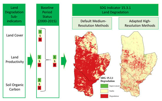
  • Does using higher resolution data (30 m) improve the delineation of LD compared to moderate-resolution data (250 m)?

2. Materials and Methods

2.1. Study Area

The study site is situated in Kiteto and Kongwa districts, located in Dodoma and Manyara regions of Central Tanzania, respectively (Figure 1). The elevation ranges between 850 and 2100 m above sea level. The study area has a hot arid steppe climate [29]. The average monthly temperature stays between 19 and 25 °C all year, and the precipitation is roughly 600 mm a year, with interannual differences of 500 to 800 mm. Large parts of northern Kiteto and more minor areas of the mountainous region in Kongwa are protected areas for nature and landscape conservation.

2.2. Materials

The SDG 15.3.1 indicator and its three LDN sub-indicators were computed using the recommended default method (DM) with Trends.Earth [30] and the adapted methods (AM) using high-resolution Landsat (and other) datasets (Table 1).
The DM (LC) map provided by the UNCCD is based on the 300 m ESA CCI LC map (Table 1). The AM utilized 30 m LC maps for 2000–2018 in the study area that the Regional Centre for Mapping of Resource for Development (RCMRD) developed. Both datasets were disaggregated into the six LC classes as defined by Intergovernmental Panel on Climate Change (IPCC), i.e., forestland, grassland, cropland, wetland, urban, and otherlands [31].
The recommended global default dataset uses the MOD-13Q1-coll6 (250 m) MODIS-NDVI products [30]. In contrast, the AM was calculated based on a 30 m resolution NDVI from a combination of Landsat 5, 7 and 8 (Table 1). The Landsat time series were accessed and analyzed using Google Earth Engine [32], based on atmospherically corrected surface reflectance collections (Table 1). The Landsat 5 and 7 data were spectrally harmonized with Landsat 8 series using linear transformation [33]. As a further step to improve the image quality, the fmask was adopted to mask out clouds and cloud shadows [34,35]. Generally, the images with cloud cover scores higher than 80% were removed. Finally, the NDVI was calculated for each image, and then the images of the same admission time were merged and clipped to the extent of the study area. As it is recommended to constrain the observation period to the growing season to reduce the number of irrelevant assets for the computation and enhance the quality of the time series [22], we used the imagery from November to June. When using Trends.Earth, there is no possibility to apply the computation to the growing season, so the DM uses the whole calendar year. In order to integrate the rainfall information, data from Climate Hazards Group InfraRed Precipitation with Station (CHIRPS) were used (Table 1).
Table 1. The datasets used for land degradation neutrality (LDN) reporting. For the land cover, the European Space Agency Climate Change Initiative (ESA-CCI) and the Regional Center for Mapping of Resources for Development (RCMDR) were used. Land productivity is based on the Moderate Resolution Imaging Spectroradiometer (MODIS) and Landsat. The precipitation is based on the Climate Hazards Group InfraRed Precipitation with Station data (CHIRPS). Lastly, the soil organic carbon content is derived from SoilGrids250m.
LDN
Sub-Indicators
MethodDataResolution/YearReference
Land CoverDefault Method (DM)ESA-CCI300 m (2000–2015)[36]
Adapted Method (AM)RCMRD30 m (2000–2018)[37]
Land ProductivityDMMOD-13Q1-coll6250 m (2000–2015)[38]
AMLandsat 530 m (2000–2013)[39]
Landsat 730 m (2000–2019)
Landsat 830 m (2013–2019)
DM/AMCHIRPS0.05 arc° (2000–2019)[40]
Soil Organic CarbonDM/AMSoilGrids250m250 m[41]
The SOC metrics were derived from the SoilGrids250m dataset [41] for the DM and the AM, as there is no national SOC database for Tanzania. SOC is measured at a depth of 30 cm and is stated as mass per area (e.g., tons per hectare (t/ha)) [22].

2.3. Methods

The calculation of the SDG 15.3.1 indicator is based on the “one out, all-out” approach (Ref. [23] and Figure 2). The three LD sub-indicators (LC change, LP decline and loss of SOC) are estimated, and if one indicator signals degradation, the LD indicator will reflect this as well. A baseline is needed to compare the progress of LDN. The baseline year (t0) was set to be 2015 and is computed as the average of the period leading up to t0 (2000–2015). The indicators are then remeasured in regular time intervals leading to 2030, and change is used to monitor the progress to accomplish LDN [20].
To calculate the indicator for the reporting year 2019 (t1), it is necessary first to assess the baseline util t0 and then calculate the change from the baseline to t1 (Figure 2). As a final step, combine both results. The details of the calculation of each indicator are explained in the following section. The three LD sub-indicators were created from satellite images using cloud-based geospatial computing. The indicators were calculated using Trends.Earth [30] and Google Earth Engine [32] for the DM and AM, respectively. As Trends.Earth currently only enables the computation for the baseline period (BP), the DM is only available from 2000 to 2015.

2.3.1. Sub-Indicator 1: Land Cover Transitions and Degradation

The first SDG 15.3.1 indicator is the LC change. To assess the LC degradation, the transitions between 2000–2015 and 2015–2018 were analyzed for the baseline and the first monitoring period (MP), respectively. To determine whether changes from one LC class to another are interpreted as degradation, a change matrix can help visualize the transitions (Table 2) based on the Good Practice Guidance by the UNCCD [31]. It is recommended to adopt this matrix for the national context. Therefore, transitions from grasslands to croplands were not considered LD for the AM to avoid tradeoff between ecosystems and food security and between nomadic and sedentary living.

2.3.2. Sub-Indicator 2: Loss of Land Productivity

LP is described as “the biological productive capacity of the land”. It is closely associated with net primary productivity [42], which can be measured directly with earth observation methods [22]. NDVI is a widely used index detecting LP [26,43,44]. The LP sub-indicator consists of three distinct components, namely trend, state and performance.
The LP trend component measures the trajectory of change in productivity over time. It is calculated at the pixel level using linear regression and the Mann Kendall significance test [22,45,46]. Positive and negative changes in NDVI indicate increasing and decreasing productivity associated with vegetation recovery and degradation, respectively. The eight most recent years of data were used to create a new distinct and significant time series that is more responsive to present land conditions. Further, following [47], we accounted for the effect of rainfall variability on vegetation productivity trends by using the rain use efficiency (RUE) method.
The LP state component represents recent changes in LP compared to the BP. The yearly NDVI mean images of the shortened BP (2000–2012) were normalized and assigned to classes from 1 to 10 based on their percentiles. To avoid annual fluctuations, contemporary values of the three-year anteceding t0 and t1 were classified in this scheme. Areas with a reduction of two or more classes were classified as degraded, while the rise by two categories was interpreted as an improvement [31].
The LP performance component examines local productivity compared to similar ecoregions defined by the unique combination of SoilGrids [41], soil taxonomy great groups and LC classes (Table 1). The 90th percentile in each ecoregion was calculated as a proxy for the maximum productivity level. The LP performance was then calculated based on the ratio of the observed mean NDVI value per pixel and the NDVImax (90th). Values below 0.5 indicate regions where the LP is low and LD may prevail [31].
The overall LP sub-indicator is calculated based on the three components mentioned earlier. As the LP trend is based on a statistically significant test, it is most influential, and its status determines LP degradation. Only if both LP status and LP performance show negative results, does the LP indicator also show degradation [22]. If only the LP state component shows degradation, this could indicate “early signs of decline” because the other indicators may not have detected the most recent LD. Further, if only performance shows degradation, there is no temporal trend, and the land is classified as “stable but stressed” [22]. In contrast to the Good Practice Guidance by UNCCD, Trends.Earth (DM) also incorporates the “early signs of decline” state component into the LP degradation [30].

2.3.3. Sub-Indicator 3: Degradation of Soil Organic Carbon

The Good Practice Guidance for the SOC sub-indicator is based on the maximum equilibrium SOC content at a location that is controlled by environmental factors such as rainfall, evaporation, solar radiation, and temperature [22]. The content can change based on three distinct change factors: First, the land-use factor represents SOC stock changes based on the type of land use. Second, the management factor reflects the management practice of the land use (e.g., grazing intensity on grasslands). Third, the input factor represents the different amounts of carbon input into the soil [22,48,49]. While the LULC change factor can be used with LC as a proxy, there are presently no sufficient datasets available to provide information about the management or the input for the other two indicators. Thus, the only indicator to assess SOC changes is the second LD indicator LC change [22].

3. Results

Three sub-indicators, namely LC transitions, LP decline, and SOC loss, were estimated to derive the SDG 15.3.1 indicator using the default and adapted methods. The patterns of each sub-indicator based on DM and AM are described in the following sections starting with the BP from 200 to 2015 for both DM and AM. The first monitoring period from 2015 to 2019 is only assessed using the AM, as the data necessary for this period are currently not available in Trends.Earth.

3.1. Sub-Indicator 1: Land Cover Transitions and Degradation

According to the DM based on the medium-resolution 300 m LC maps, over 99% of the study area remained stable in the BP (2000–2015) (Table A1). Urban areas covering less than 0.1% of the study area experienced the highest relative expansion (56%). The forestlands were the only other LC class that increased in area significantly (4.4%) in the BP.
In contrast to the DM, the AM with high-resolution (30 m) LC data revealed that 6.7% of the total area changed to a less desirable LC class, signifying LD, and only 2.3% of analyzed areas improved. The area of (semi)natural LC, such as forestlands (−19%), grasslands (−6.6%) and wetlands (0.1%), mostly declined, whereas the croplands recorded the highest spatial gain (24.2%) (Figure 3 and Table 2).
The trend observed in the BP continued in the first years of the MP (Figure 3 and Table A2). Overall, from 2015 to 2018, 3.3% of the total area was degraded during the MP, while 1.2% of the area changed to a more desirable LC. Grass- and forestlands continued to decline by 3 to 9%, respectively, while anthropogenic(-influenced) covers such as cropland and urban areas expanded. Compared to about 3000 ha forests lost per year (a) in the BP, the rate doubled to 6000 ha/a in the MP. Similarly, the changes in croplands increased from 6000 ha/a in 2000–2015 to 7500 ha/a in 2015–2018.

3.2. Sub-Indicator 2: Loss of Land Productivity

The DM revealed that the LP sub-indicator showed degradation in 71.1% of the area during the BP from 2000 to 2015 (Table 3). The LP component trend showed “decline” in 26.8% of the area (Figure A1A). Another 44.3% of the study area showed “early signs of decline” (LP component state, Figure A2A), and the rest (28.9%) remained stable (Figure 4A). According to DM, croplands were most affected (48.4%) by LP decline in 2000–2015 (Figure 5). Forestlands with only about 11.7% marked as degraded were less affected compared to their actual LC share (Figure 5).
Based on the AM applied between 2000 and 2015, the final composite indicators of LP decline revealed that 8.2% of the study area was degraded between 2000 and 2015 (Table 3). This is nearly entirely based on the 8.2% “decline” of the LP trend component (Figure A1B). Further, 9.1% and 1.4% of the study area were marked as showing “early signs of decline” (Figure A2B) and “stable but stressed” areas (Figure A3B), respectively (Figure 4B). Grass- and croplands accounted for 43.5% and 42% of the degraded area (Figure 5). The decline in forestlands was, in turn, detected only on 2.6% of the total degraded area.
LP declined over 12.2% of the study area during the MP from 2015 to 2019 (Figure 4C). With an increase from 9.1% up to 17% of the area, the share of areas with “early signs of decline” (state component) was higher than during the BP (Figure A2). The area where LP was improving was reduced from 855 to 171 km2 compared to the BP.

3.3. Sub-Indicator 3: Degradation of Soil Organic Carbon

Soil organic carbon was not directly computed but rather assessed through LC classes’ alteration and the related change factors [49]. SOC did not change significantly with the DM during the BP from 2000 to 2015: 99.9% of the land did not change the in SOC content by more than 10% (Table 4). Changes in the individual LC classes were also neglectable.
In contrast to DM, the AM approach revealed that during the BP of 2000–2015, 8.4% of the land was degraded due to SOC diminishment, while 2.1% increased in SOC content (Figure 6). The average SOC stock declined from 51.2 to 50.2 t/ha in 2015, losing 1,592,423 t of carbon over 16 years (Table 4). Forestlands had significantly higher SOC stocks (62.2 t/ha) at t0 than the other LC classes. Based on the transitions in LC, the amount of SOC in forests dropped by 19%, while SOC under agricultural use increased by 25.1%.
In the MP, the SOC content experienced significant losses on 3.7% of the land. The same trend was observed in other LC classes (forest-, grass- and wetlands) that gradually lost SOC in the MP (Table 4).

3.4. Combined Sustainable Development Indicator 15.3.1 for the Baseline and First Monitoring Period

During the BP from 2000 to 2015, the DM method identified 71.1% of KK’s area as degraded and only as 0.5% improved (Figure 7A). This result is mainly caused by the sub-indicator LP, while the two other indicators LC and SOC showed nearly no degradation. The LP degradation was mainly driven by the state component of LP in 70.3% of the total area.
On the contrary, during the BP, the AM showed that 16.4% of the area was degraded and 2.7% improved (Figure 7B). The distinct sub-indicators influenced the final indicator more evenly with 52.4%, 50% and 31.7% by SOC, LP and LC, respectively, compared to the DM.
The AM for the first MP (2015–2019) showed that 16% of the total area was degraded, 1.5% improved and more than 82% remained stable (Figure 7C). Forests and grasslands were the least affected among LC classes. Croplands (38%) and wetlands (7%) experienced the most degradation between 2015 and 2019. Over three-fourths of the degradation was driven by the LP sub-indicator, whereas LC and SOC only contributed 20% and 23% to LD, respectively.

3.5. Combined Sustainable Development Indicator 15.3.1 over 20 Years Using the AM

Over the whole period of 20 years (2000–2019), which results in the SDG 15.3.1 indicator at timestep t1, 27.7% of KK was degraded, and 2.8% of KK improved (Figure 8A). Thus, the LD was widespread across the two studied districts and formed several LD clusters (Figure 7B,C). The degradation was not equally distributed over the study area: the biggest LD hotspots were Central and Western Kiteto, as well as Western Kongwa (Figure 8A). Even though the land covered by forests decreased and the land covered by crops increased from 2015 to 2018, the degraded proportion changed conversely as follows: The degraded area covered by forests increased to 3.9%, while the area covered by crops sank to 41.9%. While SOC’s degraded area only changed slightly, the relative contribution sank from 50 to 30% (Figure 8B). The degraded area, which is solely influenced by LP, rose over 50% and interplayed with others over 70%.

4. Discussion

The presented study is the first in Africa to support the monitoring of the SDG 15.3.1 indicator using fine-spatial-resolution (30 m) satellite time series data for LD assessment. This is a key contribution considering that previous studies used 250 m to 8 km resolution data [24,26,50] for LP sub-indicator monitoring, unlike our study that utilized long-term Landsat time series for SDG 15.3.1 monitoring. Furthermore, it is the first sub-national study that assesses the SDG 15.3.1 indicator in Tanzania for the BP and includes the MP until 2019. The first 4 out of 15 years of the SDG time frame are assessed and could help identify hotspot areas for targeting the appropriate measures to combat LD in the study area.
The presented LD assessment in KK districts confirmed that the LD problem is acute in Tanzania. The Tanzanian target is to achieve LDN by 2030 [24]. Both KK are part of declared LD hotspot regions, which need to improve 25% of the area based on the status at t0. According to our analysis, only 2.7% of the land area has improved and 27.7% is degraded. Next to the (sub)national targets, there are also specific targets to avoid, minimize and reverse LD in Tanzania [24]. Among others, about half of the current national forest area should be restored, 50% of the national croplands should improve LP and the SOC content in croplands should rise to 54.5 t/ha [51]. Despite these more specific and ambitious targets, our results show a negative trend in all LD sub-indicators analyzed, suggesting that more efforts are needed to combat LD in the study area.
Precisely, instead of restoring forest areas, even more trees were cut over 19 years (14.7% to 10.9% tree cover). In croplands, LP degradation was above average, while the SOC content in croplands improved marginally. A possible explanation could be that restoration attempts using SLM practices had not yet shown effects, because it takes several years for the change to be monitored remotely [52,53]. Moreover, it takes decades for SOC to change [49,54]. Hence, it is of paramount importance to prioritize the detected LD hotspots for rehabilitation and SLM practices to reverse LD processes.
There are currently no sub-national studies for KK districts. With around 27% of the area in KK being degraded, it is less affected by LD compared to national assessments found in [2,3] or [11]. However, the comparison with these studies is difficult, as they used different monitoring periods (ending in the 2000s and 2016) and only a subset of the methodology (LP trend) and coarse resolution imagery (i.e., 8 km AVHRR data). This suggests that our study brought LD assessment in Tanzania one step further by assessing three components of LD according to the SDG 15.3.1 indicator. Further, using significantly higher spatial resolution, spatial datasets allowed us to reveal spatial patterns of LD beyond pixel sizes of 8 km [2,3,11] or 1 km [24].
Our study compared the results of the LD assessments based on default UNCCD-suggested datasets (250 m MODIS data used for LP sub-indicator and 300 m ESA CCI LC maps) and customized relatively high-resolution datasets (30 m Landsat data used for the LP sub-indicator and 30 m RCMRD LC maps). The resulting differences between LD estimates based on DM and AM were striking and could be primarily attributed to the difference in the pixel size of 6.25 ha (MODIS) versus 0.09 ha (Landsat), which could be critical in specific areas where fine LD patterns prevailed. This finding is confirmed by several studies highlighting the importance of using high-resolution imagery to detect LD, especially on heterogeneous landscapes, such as KK districts, dominated by heterogenous small-scale farms [50,55,56]. Recent studies that used ground-truth data for validation showed that using Landsat data for the LC sub-indicator captured LD better than using ESA-based 300 m datasets [50]. Nevertheless, certain factors could have impacted the AM, such as the scan-line failure in Landsat ETM+ data. To reduce the potential negative influence of this on our analysis, we applied several preprocessing steps confirmed to be effective in similar studies [56].
NDVI was applied in this study, although it was affected by soil brightness in areas with low vegetation cover. Other vegetation indices, such as MSAVI or MSAVI2, are less sensitive to soil optical properties in less vegetated areas and, therefore, can be used to detect a decline in vegetation productivity [57]. However, the alternative indices have significantly better results than NDVI only in areas where bare soils prevail. Further, Tüshaus et al. [58] compared NDVI with the Soil-Adjusted Vegetation Index (SAVI) and MERIS-based Terrestrial Chlorophyll Index (MTCI). The results indicated only little differences between the different vegetation indices. Nevertheless, the impact of different vegetation indices on the estimated LDN sub-indicators can be further tested.
Furthermore, our results pointed out that the ESA CCI LC did not reflect significant LC changes during the BP in KK districts. Other local estimates, such as the National Forest Resources Monitoring and Assessment of Tanzania Mainland [21] or Tanzanian Forest Reference Emission Level [59], suggest a change rate that is three to twenty times higher, respectively, for a similar period analyzed. Our result is in line with the study of Kimaro et al. [60], who investigated the LC change for the study area from 1987 to 2010. Their study indicated that the LC change was already in progress over 30 years ago with heavy declines in (semi)-natural landscapes. This suggests that our research offers advancement of sub-national assessment of LD in heterogeneous landscapes.
Our study revealed that the LP sub-indicator impacted LD in the study area the most (by 50%) using the AM. The remaining half is affected by SOC, LC, or by the combination of more than one sub-indicator. On the other hand, the LD indicator using the DM is nearly solely affected by the LP sub-indicator, which is primarily driven by the state component. This suggests two things: First, our AM is better suited to reflect the ongoing multidimensional degradation in KK districts. Second, even if the ongoing LULC change stops, the degradation will not halt because of the decline in LP.
This is well reflected in croplands, which were the worst affected land cover class, not only in LP decline but also in SOC loss. Due to the continuous cultivation of the agricultural lands combined with overgrazing and little fertilizer inputs, the crop yields in the study area are reportedly low, caused by the limited availability of soil nutrients and organic matter content [18]. Another study that assessed LD in Kenya in similar environmental and land use settings found that croplands experienced the highest decline in LP, indicating that unsustainable farming practices are widespread throughout Eastern Africa [26]. This has serious consequences, as already 30% of the Tanzanian population are undernourished [16], and the yield gap for the main crops needs to be closed for the population to sustain itself in the coming decades [61].
The soils in KK districts lost 1.6 million t of SOC due to LULC change from 2000–2018, according to our study. This is especially dire, as SOC is vital for soil quality and is a key ecosystem indicator [62]. The study by van der Esch et al. [63] suggests that due to LULC change, 27 Gt of SOC will be further lost globally by 2050, mainly in sub-Saharan Africa. Studies conducted in Tanzania found that higher SOC values on the farm level resulted in financial benefits for the farmers [64]. Thus, increasing SOC via SLM practices would not only improve farmers’ living conditions but also allow slowing down ongoing SOC degradation.
In contrast to the LP and LC sub-indicators, which have a continuous basis with Landsat and Sentinel missions [65] and for which there are also further high-resolution maps available [66], the SOC sub-indicator still lacks good spatial and temporal coverage. Further, there are currently no sufficient datasets available to provide information about the management or the input for the SOC indicator. Thus, the SOC change is only approximated by the LC change sub-indicator, leading to a misbalance towards the LULC change in the overall SDG 15.3.1 indicator. At the moment of the analysis, the high spatial resolution SOC data by Innovative Solutions for Decision Agriculture (iSDA) based on [67] were not available. Further work should thus address this limitation and incorporate per availability high-resolution SOC data in the analysis, as well as conducting field validation of both approaches. At the beginning of 2021, the UNCCD updated the first version of the SDG 15.3.1 good practice guidance and innovated the methodology [68]. Future studies should therefore adopt this new approach in conjunction with newly available datasets.
The improvement of the subnational analysis with freely available data, the use of cloud computing platforms, and the source code’s availability to perform LD assessment present an opportunity to upscale the analysis further and transfer the methods to other study areas.

5. Conclusions

The presented study demonstrates the potential of earth observation for LD monitoring with high spatial resolution data and uses cloud computing approaches with Google Earth Engine, and it improves the measurement of the SDG 15.3.1 indicator in the study area in Tanzania up until 2015 and 2019 at two different levels of spatial detail. Our study thus offers advancement of sub-national assessments of land degradation (LD) in heterogeneous landscapes. The improvement of the sub-national analysis with high-resolution data, the use of cloud computing platforms and the provision of the source code used here to perform LD assessment should encourage a transfer of the here presented approach to other study areas and/or the upscaling of the results of this study to the national level.
For this, we compared two approaches of assessing the SDG indicator 15.3.1 in Kiteto and Kongwa districts of Tanzania. The first method applied the global default (DM) medium resolution datasets proposed by the UNCCD for monitoring LD for the baseline period (BP, 2000–2015). The second method, the adapted method (AM), applied local land cover 30 m maps and 30 m Landsat to monitor LD for the baseline and the first monitoring period (MP, 2015–2019). The LD assessment for the BP reveals large differences between the DM and AM. Using the DM, nearly all degraded area stems from the LP sub-indicator based on 250 m MODIS imagery. In contrast, the degradation was less than 1% for the LC and SOC change sub-indicators, calculated based on ESA CCI LC (300 m) maps. The LD captured by the AM based on Landsat time series and 30 m LC data was evenly distributed between the three sub-indicators and revealed LD on 27.7% of the area. We, therefore, concluded that the results derived from medium-resolution datasets are likely to over- and underestimate the LD for different sub-indicators and, thus, might misinform policy- and decision-makers and land managers if used operationally. Further, our study concluded that the local datasets and high-resolution imagery are essential to capture subtle changes within the heterogeneous landscape in semiarid central Tanzania.
Our results confirmed that LD is currently ongoing in the study area. The LD did not halt after 2015 but spread further across the districts and formed several severe LD clusters. Therefore, to achieve the national LDN targets, it is crucial to address the most important LD causes, such as overgrazing and unsustainable farming in the study area. The application of SLM practices would enhance the low LP in croplands and prevent LULC change in KK districts.
Further work should incorporate high-resolution SOC data in the analysis and conduct field validation of LD assessments resulting from both approaches.

Author Contributions

Conceptualization, methodology, software and writing—original draft preparation, J.R.; writing—review and editing, J.R., G.G., F.M. and O.D.; visualization, J.R. and G.G.; supervision, F.M. and O.D.; funding acquisition, F.M. All authors have read and agreed to the published version of the manuscript.

Funding

This research was funded by the United States Agency for International Development, grant number AID-BFS-G-11-00002.

Data Availability Statement

The Google Earth Engine code can be found online on https://github.com/JAReith/SDG15.3.1.

Acknowledgments

The authors thank the German Academic Exchange Service for the generous funding by the PROMOS-program and the financial support by the International Institute for Tropical Agriculture for the fieldwork in Tanzania.

Conflicts of Interest

The authors declare no conflict of interest. The funders had no role in the design of the study; in the collection, analyses, or interpretation of data; in the writing of the manuscript, or in the decision to publish the results.

Appendix A

Table A1. Land cover transition matrix (2000–2015) based on the default methods (DM). Green, beige and brown colors indicate improving, stable and declining conditions of land cover categories, respectively. The area in km2 and the possible cause of the land cover transition are indicated in the matrix. The change is based on the moderate-resolution land cover dataset.
DM Land Cover Category in 2015 (km2)
ForestlandGrasslandCroplandWetlandUrbanOtherland2000 Total (km2)
DM Land cover category in 2000 (km2)ForestlandStable
2810.18
Vegetation loss
3,83
Deforestation
0.68
Inundation
0
Deforestation
0.49
Vegetation loss
0
2815.19
GrasslandAfforestation
127.43
Stable
6976.03
Agricultural expansion
18.72
Inundation
0.74
Urban expansion
0
Vegetation loss
0
7122.92
CroplandAfforestation
3.09
Withdrawal of agriculture
4.2
Stable
6606.86
Inundation
0
Urban expansion
0.25
Vegetation loss
0
6614.40
WetlandWoody encroachment
0
Waterbody drainage
0
Waterbody drainage
0
Stable
537.22
Waterbody drainage
0.12
Waterbody drainage
0
537.34
UrbanAfforestation
0
Vegetation establishment
0
Agricultural expansion
0
Wetland establishment
0
Stable
1.54
Withdrawal of settlements
0
1.54
OtherlandAfforestation
0
Vegetation establishment
0
Agricultural expansion
0
Wetland establishment
0
Urban expansion
0
Stable
0
0
2015 total (km2)2940.716984.066626.25537.962.41017,091.40
Table A2. Land cover transition matrix in km2 (2015–2018) based on the adapted methods (AM). Green, beige and brown colors indicate improvement, stable and decline of land cover category, respectively. The area and the possible cause of the land cover transition are indicated in the matrix. The change is based on the high-resolution land cover dataset.
AM Land Cover Category in 2018 (km2)
ForestlandGrasslandCroplandWetlandUrbanOtherland2015 Total (km2)
AM Land cover category in 2015 (km2)ForestlandStable
1819.5
Vegetation loss
89.5
Deforestation
94.2
Inundation
19.3
Deforestation
5.4
Vegetation loss
13.1
2041
GrasslandAfforestation
26.2
Stable
6993
Agricultural expansion
368.1
Inundation
77
Urban expansion
22.7
Vegetation loss
77
7563.9
CroplandAfforestation
9.3
Withdrawal of agriculture
175.4
Stable
4602.4
Inundation
50.9
Urban expansion
23
Vegetation loss
64.6
4925.6
WetlandWoody encroachment
0.7
Waterbody drainage
5.5
Waterbody drainage
7.4
Stable
173.7
Waterbody drainage
0.8
Waterbody drainage
4.7
192.9
UrbanAfforestation
0.1
Vegetation establishment
2.2
Agricultural expansion
10
Wetland establishment
0.6
Stable
196.7
Withdrawal of settlements
1.4
211
OtherlandAfforestation
2.7
Vegetation establishment
55.7
Agricultural expansion
69.7
Wetland establishment
30.6
Urban expansion
10.1
Stable
1988.3
2157
2018 total (km2)1858.47321.45151.7352.2258.72149.117,091.4
Figure A1. The land productivity component trend generated using (A) the default approach with MODIS imagery, (B) the adapted approach with Landsat imagery for the baseline period, and (C) the adopted approach with Landsat imagery for the monitoring period 2015–2019.
Remotesensing 13 01754 g0a1
Figure A2. The land productivity component state generated using (A) the default approach with MODIS imagery, (B) the adapted approach with Landsat imagery for the baseline period, and (C) the adopted approach with Landsat imagery for the monitoring period 2015–2019.
Remotesensing 13 01754 g0a2
Figure A3. The land productivity component performance generated using (A) the default approach with MODIS imagery, (B) the adapted approach with Landsat imagery for the baseline period, and (C) the adopted approach with Landsat imagery for the monitoring period 2015–2019.
Remotesensing 13 01754 g0a3

References

  1. UNCCD. Elaboration of an International Convention to Combat Desertification in Countries Experiencing Serious Drought and/or Desertification, Particularly in Africa; UNCCD: Paris, France, 1994. [Google Scholar]
  2. Le, Q.B.; Nkonya, E.; Mirzabaev, A. Biomass productivity-based mapping of global land degradation hotspots. In Economics of Land Degradation and Improvement; Nkonya, E., Mirzabaev, A., von Braun, J., Eds.; Springer Open: Cham, Switzerland, 2016; Volume 24, pp. 55–84. ISBN 978-3-319-19167-6. [Google Scholar]
  3. Bai, Z.; Dent, D.L.; Olsson, L.; Schaepman, M.E. Proxy Global Assessment of Land Degradation. Soil Use Manag. 2008, 24, 223–234. [Google Scholar] [CrossRef]
  4. Dubovyk, O. The Role of Remote Sensing in Land Degradation Assessments: Opportunities and Challenges. Eur. J. Remote Sens. 2017, 50, 601–613. [Google Scholar] [CrossRef]
  5. Barbier, E.B.; Hochard, J.P. Land Degradation and Poverty. Nat. Sustain. 2018, 1, 623–631. [Google Scholar] [CrossRef]
  6. IPBES. The IPBES Assessment Report on Land Degradation and Restoration; 2018. Bonn: Intergovernmental Science-Policy Platform on Biodiversity and Ecosystem Services (IPBES). Available online: https://www.ipbes.net/assessment-reports/ldr (accessed on 24 April 2021).
  7. ELD Initiative. The Value of Land: Prosperous Lands and Positive Rewards through Sustainable Land Management; Stewart, N., Ed.; Economics of Land Degradation Initiative: Bonn, Germany, 2015; ISBN 978-92-808-6061-0. [Google Scholar]
  8. IPCC Climate Change and Land. IPCC Special Report on Climate Change, Desertification, Land Degradation, Sustainable Land Management, Food Security, and Greenhouse Gas Fluxes in Terrestrial Ecosystems; IPCC: Geneve, Switzerland, 2019. [Google Scholar]
  9. UNCCD Report of the Conference of the Parties on Its Seventeenth Session, Held in Durban from 28 November to 11 December 2011: Part Two: Action Taken by the Conference of the Parties at Its Eleventh Session: ICCD/COP(11)/23/Add.1. 2013. Available online: https://unfccc.int/resource/docs/2011/cop17/eng/09.pdf (accessed on 24 April 2021).
  10. UN Transforming Our World: The 2030 Agenda for Sustainable Development; 2015. Available online: https://stg-wedocs.unep.org/bitstream/handle/20.500.11822/11125/unepswiosm1inf7sdg.pdf?sequence=1 (accessed on 24 April 2021).
  11. Kirui, O.K.; Mirzabaev, A.; von Braun, J. Assessment of Land Degradation ‘on the Ground’ and from ‘Above’. SN Appl. Sci. 2021, 3, 318. [Google Scholar] [CrossRef]
  12. FAO The Global Forest Resources Assessment 2015: Desk Reference; Food and Agriculture Organization of the United Nations: Rome, Italy, 2015.
  13. Kirui, O.K. Economics of land degradation and improvement in tanzania and malawi. In Economics of Land Degradation and Improvement; Nkonya, E., Mirzabaev, A., von Braun, J., Eds.; Springer Open: Cham, Switzerland, 2016; Volume 22, pp. 609–649. ISBN 978-3-319-19167-6. [Google Scholar]
  14. FAO. NBS Tanzania: CountrySTAT; Food and Agriculture Organization of the United Nations: Rome, Italy; National Bureau of Statistics: Dar es Salam, Tanzania, 2020. Available online: http://tanzania.countrystat.org/home/en/ (accessed on 24 April 2021).
  15. NBS National Environment Statistics Report, 2017: Tanzania Mainland; National Bureau of Statistics: Dar es Salam, Tanzania, 2018.
  16. FAO. FAO Stat Tanzania; Food and Agriculture Organization of the United Nations: Rome, Italy, 2019; Available online: http://www.fao.org/faostat/en/#country/215 (accessed on 24 April 2021).
  17. Wheeler, T.; von Braun, J. Climate Change Impacts on Global Food Security. Science 2013, 341, 508–513. [Google Scholar] [CrossRef]
  18. Kimaro, A.A.; Mpanda, M.; Meliyo, J.L.; Ahazi, M.; Ermias, B.; Shepherd, K.D.; Coe, R.; Okori, P.; Mowo, J.G.; Bekunda, M. Soil Related Constraints for Sustainable Intensification of Cereal-Based Systems in Semi-Arid Central Tanzania. In Proceedings of the Tropentag 2015: Management of Land Use Systems for Enhanced Food Security: Conflicts, Controversies and Resolutions, Berlin, Germany, 16–18 September 2015; Tielkes, E., Ed.; Cuvillier Verlag: Göttingen, Germany, 2015; p. 675. ISBN 978-3-7369-9092-0. [Google Scholar]
  19. Liniger, H.; Harari, N.; van Lynden, G.; Fleiner, R.; de Leeuw, J.; Bai, Z.; Critchley, W. Achieving Land Degradation Neutrality: The Role of SLM Knowledge in Evidence-Based Decision-Making. Environ. Sci. Policy 2019, 94, 123–134. [Google Scholar] [CrossRef]
  20. Orr, B.J.; Cowie, A.L.; Castillo, V.M.; Chasek, P.; Crossman, N.D.; Erlewein, A.; Louwagie, G.; Maron, M.; Metternicht, G.I.; Minelli, S.; et al. Scientific Conceptual Framework for Land Degradation Neutrality: A Report of the Science-Policy Interface; United Nations Convention to Combat Desertification (UNCCD): Bonn, Germany, 2017; pp. 1–98. [Google Scholar]
  21. Caspari, T.; van Lynden, G.; Bai, Z. Land Degradation Neutrality: An Evaluation of Methods; Ehlers, K., Ed.; Federal Ministry for the Environment, Nature Conservation, Building and Nuclear safety, Umweltbundesamt: Dessau-Roßlau, Germany, 2015.
  22. URT. URT Land Degradation Neutrality Target Setting Programme Report; The United Republic of Tanzania (URT): Dar es Salam, Tanzania, 2018.
  23. Giuliani, G.; Chatenoux, B.; Benvenuti, A.; Lacroix, P.; Santoro, M.; Mazzetti, P. Monitoring Land Degradation at National Level Using Satellite Earth Observation Time-Series Data to Support SDG15—Exploring the Potential of Data Cube. Big Earth Data 2020, 5, 1–20. [Google Scholar] [CrossRef] [Green Version]
  24. Gichenje, H.; Godinho, S. Establishing a Land Degradation Neutrality National Baseline through Trend Analysis of GIMMS NDVI Time-Series. Land Degrad. Dev. 2018, 29, 2985–2997. [Google Scholar] [CrossRef]
  25. Frederique, M.; Agnes, B.; Louise, L.; Clovis, G. Sensitivity Analysis of Land Productivity Change Calculation in Mozambique. In Proceedings of the IGARSS 2019—2019 IEEE International Geoscience and Remote Sensing Symposium, Yokohama, Japan, 28 July 2019; pp. 1633–1636. [Google Scholar]
  26. Anderson, K.; Ryan, B.; Sonntag, W.; Kavvada, A.; Friedl, L. Earth Observation in Service of the 2030 Agenda for Sustainable Development. Geo Spat. Inf. Sci. 2017, 20, 77–96. [Google Scholar] [CrossRef]
  27. Beck, H.E.; Zimmermann, N.E.; McVicar, T.R.; Vergopolan, N.; Berg, A.; Wood, E.F. Present and Future Köppen-Geiger Climate Classification Maps at 1-Km Resolution. Sci. Data 2018, 5, 180214. [Google Scholar] [CrossRef] [Green Version]
  28. Conservation International TRENDS.EARTH. Trends.Earth Documentation: Release 0.66; TRENDS.EARTH: Arlington, GA, USA, 2019. [Google Scholar]
  29. Sims, N.C.; England, J.R.; Newnham, G.J.; Alexander, S.; Green, C.; Minelli, S.; Held, A. Developing Good Practice Guidance for Estimating Land Degradation in the Context of the United Nations Sustainable Development Goals. Environ. Sci. Policy 2019, 92, 349–355. [Google Scholar] [CrossRef]
  30. Gorelick, N.; Hancher, M.; Dixon, M.; Ilyushchenko, S.; Thau, D.; Moore, R. Google Earth Engine: Planetary-Scale Geospatial Analysis for Everyone. Remote Sens. Environ. 2017, 202, 18–27. [Google Scholar] [CrossRef]
  31. Roy, D.P.; Kovalskyy, V.; Zhang, H.K.; Vermote, E.F.; Yan, L.; Kumar, S.S.; Egorov, A. Characterization of Landsat-7 to Landsat-8 Reflective Wavelength and Normalized Difference Vegetation Index Continuity. Remote Sens. Environ. 2016, 185, 57–70. [Google Scholar] [CrossRef] [Green Version]
  32. Foga, S.; Scaramuzza, P.L.; Guo, S.; Zhu, Z.; Dilley, R.D.; Beckmann, T.; Schmidt, G.L.; Dwyer, J.L.; Joseph Hughes, M.; Laue, B. Cloud Detection Algorithm Comparison and Validation for Operational Landsat Data Products. Remote Sens. Environ. 2017, 194, 379–390. [Google Scholar] [CrossRef] [Green Version]
  33. Zhu, Z.; Woodcock, C.E. Continuous Change Detection and Classification of Land Cover Using All Available Landsat Data. Remote Sens. Environ. 2014, 144, 152–171. [Google Scholar] [CrossRef] [Green Version]
  34. Sims, N.C.; Green, C.; Newnham, G.J.; England, J.R.; Held, A.; Wulder, M.; Herold, M.; Cox, S.J.D.; Huete, A.R.; Kuma, L.; et al. Good Practice Guidance: SDG Indicator 15.3.1: Proportion of Land That Is Degraded over Total Land Area, Version 1.0; United Nations Convention to Combat Desertification (UNCCD): Bonn, Germany, 2017. [Google Scholar]
  35. ESA. Land Cover CCI Product User Guide Version 2. Tech. Rep. 2017. Available online: http://www.esa-landcover-cci.org/?q=node/199 (accessed on 24 April 2021).
  36. RCMRD Land Use Land Cover and Change Mapping Service. Available online: https://rcmrd.org/servir-land-use-land-cover-and-change-mapping-service (accessed on 30 March 2021).
  37. USGS MOD13Q1 MODIS/Terra Vegetation Indices 16-Day L3 Global 250m SIN Grid V006. U.S. Geological Survey, Sioux Falls, United States of America. 2015. Available online: https://lpdaac.usgs.gov/products/mod13q1v006/ (accessed on 30 March 2021).
  38. Wulder, M.A.; Loveland, T.R.; Roy, D.P.; Crawford, C.J.; Masek, J.G.; Woodcock, C.E.; Allen, R.G.; Anderson, M.C.; Belward, A.S.; Cohen, W.B.; et al. Current Status of Landsat Program, Science, and Applications. Remote Sens. Environ. 2019, 225, 127–147. [Google Scholar] [CrossRef]
  39. Funk, C.; Peterson, P.; Landsfeld, M.; Pedreros, D.; Verdin, J.; Shukla, S.; Husak, G.; Rowland, J.; Harrison, L.; Hoell, A.; et al. The Climate Hazards Infrared Precipitation with Stations—A new Environmental Record for Monitoring Extremes. Sci Data. 2015, 2, 150066. [Google Scholar] [CrossRef] [PubMed] [Green Version]
  40. Hengl, T.; Mendes de Jesus, J.; Heuvelink, G.B.M.; Ruiperez Gonzalez, M.; Kilibarda, M.; Blagotić, A.; Shangguan, W.; Wright, M.N.; Geng, X.; Bauer-Marschallinger, B.; et al. SoilGrids250m: Global Gridded Soil Information Based on Machine Learning. PLoS ONE 2017, 12, e0169748. [Google Scholar] [CrossRef] [PubMed] [Green Version]
  41. Cowie, A.L.; Orr, B.J.; Castillo Sanchez, V.M.; Chasek, P.; Crossman, N.D.; Erlewein, A.; Louwagie, G.; Maron, M.; Metternicht, G.I.; Minelli, S.; et al. Land in Balance: The Scientific Conceptual Framework for Land Degradation Neutrality. Environ. Sci. Policy 2018, 79, 25–35. [Google Scholar] [CrossRef]
  42. Clark, D.A.; Brown, S.; Kicklighter, D.W.; Chambers, J.Q.; Thomlinson, J.R.; Ni, J. Measuring Net Primary Production in Forests: Concepts and Field Methods. Ecol. Appl. 2001, 11, 356. [Google Scholar] [CrossRef]
  43. Ivits, E.; Cherlet, M. Land-Poductivity Dnamics Twards Itegrated Asessment of Land Degradation at Global Scales; EUR, Scientific and Technical Research Series; Publications Office: Luxembourg, 2016; Volume 26052, ISBN 978-92-79-32354-6. [Google Scholar]
  44. Landmann, T.; Dubovyk, O. Spatial Analysis of Human-Induced Vegetation Productivity Decline over Eastern Africa Using a Decade (2001–2011) of Medium Resolution MODIS Time-Series Data. Int. J. Appl. Earth Obs. Geoinf. 2014, 33, 76–82. [Google Scholar] [CrossRef]
  45. Mann, H.B. Nonparametric Tests against Trend. Econometrica 1945, 13, 245. [Google Scholar] [CrossRef]
  46. Kendall, M.G. Rank Correlation Methods; C. Griffin: Glasgow, UK, 1948. [Google Scholar]
  47. Le Houerou, H.N. Rain Use Efficiency: A Unifying Concept in Arid-Land Ecology. J. Arid Environ. 1984, 7, 213–247. [Google Scholar]
  48. IPCC 2006 IPCC Guidelines for National Greenhouse Gas Inventories; Eggleston, H.S.; Miwa, K.; Srivastava, N.; Tanabe, K. (Eds.) Institute for Global Environmental Strategies (IGES): Hayama, Japan, 2008. [Google Scholar]
  49. Mattina, D.; Erdogan, H.E.; Wheeler, I.; Crossman, N.; Minelli, S.; Cumani, R. Default Data: Methods and Interpretation: A Guidance Document for the 2018 UNCCD Reporting; United Nations Convention to Combat Desertification (UNCCD): Bonn, Germany, 2018. [Google Scholar]
  50. Akinyemi, F.O.; Ghazaryan, G.; Dubovyk, O. Assessing UN Indicators of Land Degradation Neutrality and Proportion of Degraded Land over Botswana Using Remote Sensing Based National Level Metrics. Land Degrad. Dev. 2020. [Google Scholar] [CrossRef]
  51. URT. URT Voluntary Land Degradation Neutrality Targets and Associated Measures of the United Republic of Tanzania; The United Republic of Tanzania (URT): Dar es Salam, Tanzania, 2018.
  52. GEF Value for Money Analysis for the Land Degradation projects of the GEF; Independent Evaluation Office, Global Environment Facility: Washington, DC, USA, 2016.
  53. Gonzalez-Roglich, M.; Zvoleff, A.; Noon, M.; Liniger, H.; Fleiner, R.; Harari, N.; Garcia, C. Synergizing Global Tools to Monitor ProgressTtowards Land Degradation Neutrality: Trends.Earth and the World Overview of Conservation Approaches and Technologies Sustainable Land Management Database. Environ. Sci. Policy 2019, 93, 34–42. [Google Scholar] [CrossRef]
  54. Bernoux, M.; Feller, C.; Cerri, C.C.; Eschenbrenner, V.; Cerri, C.E.P. Soil carbon sequestration. In Soil Erosion and Carbon Dynamics; Advances in Soil Science; Roose, E., Lal, R., Feller, C., Barthes, B., Stewart, B., Eds.; CRC/Taylor & Francis: Boca Raton, FL, USA, 2006; pp. 13–22. ISBN 978-1-56670-688-9. [Google Scholar]
  55. Fiorillo, E.; Maselli, F.; Tarchiani, V.; Vignaroli, P. Analysis of Land Degradation Processes on a Tiger Bush Plateau in South West Niger Using MODIS and LANDSAT TM/ETM+ Data. Int. J. Appl. Earth Obs. Geoinf. 2017, 62, 56–68. [Google Scholar] [CrossRef]
  56. Venter, Z.S.; Scott, S.L.; Desmet, P.G.; Hoffman, M.T. Application of Landsat-Derived Vegetation Trends over South Africa: Potential for Monitoring Land Degradation and Restoration. Ecol. Indic. 2020, 113, 106206. [Google Scholar] [CrossRef]
  57. Montandon, L.M.; Small, E.E. The Impact of Soil Reflectance on the Quantification of the Green Vegetation Fraction from NDVI. Remote Sens. Environ. 2008, 112, 1835–1845. [Google Scholar] [CrossRef]
  58. Tüshaus, J.; Dubovyk, O.; Khamzina, A.; Menz, G. Comparison of Medium Spatial Resolution ENVISAT-MERIS and Terra-MODIS Time Series for Vegetation Decline Analysis: A Case Study in Central Asia. Remote Sens. 2014, 6, 5238–5256. [Google Scholar] [CrossRef]
  59. URT. URT Tanzania’s Forest Reference Emission Level Submission to the UNFCCC; The United Republic of Tanzania (URT): Dar es Salam, Tanzania, 2017.
  60. Kimaro, A.A.; Weldesmayat, S.G.; Mpanda, M.; Swai, E.; Kayeye, H.; Nyoka, B.I.; Majule, A.E.; Perfect, J.; Kundhlade, G. Final Technical Report for the Jumpstrat Projects: Evidence-Based Scaling-up of Evergreen Agriculture for Increasing Crop Productivity, Fodder Supply and Resilience of the Maize-Mixed and Agro-Pastoral Farming Systems in Tanzania and Malawi; World Agroforestry Centre: Nairobi, Kenya, 2012. [Google Scholar]
  61. van Ittersum, M.K.; van Bussel, L.G.J.; Wolf, J.; Grassini, P.; van Wart, J.; Guilpart, N.; Claessens, L.; de Groot, H.; Wiebe, K.; Mason-D’Croz, D.; et al. Can Sub-Saharan Africa Feed Itself? Proc. Natl. Acad. Sci. USA 2016, 113, 14964–14969. [Google Scholar] [CrossRef] [PubMed] [Green Version]
  62. Chotte, J.-L.; Aynekulu, E.; Cowie, A.L.; Campbell, E.; Vlek, P.; Lal, R.; Kapovic-Solomun, M.; von Maltitz, G.P.; Kust, G.; Barger, N.; et al. Realising the Carbon Benefits of Sustainable Land Management Practices: Guidelines for Estimation of Soil Organic Carbon in the Context of Land Degradation Neutrality Planning and Monitoring: A Report of the Science-Policy Interface; United Nations Convention to Combat Desertification (UNCCD): Bonn, Germany, 2019. [Google Scholar]
  63. van der Esch, S.; ten Brink, B.; Stehfest, E.; Bakkenes, M.; Sewell, A.; Bouwman, A.; Meijer, J.; Westhoek, H.; van den Berg, M.; van den Born, G.J.; et al. Exploring Future Changes in Land Use and Land Condition and the Impacts on Food, Water, Climate Change and Biodiversity: Scenarios for the UNCCD Global Land Outlook; Policy Report; PBL Netherlands Environmental Assessment Agency: The Hague, The Netherlands, 2017. [Google Scholar]
  64. Bhargava, A.K.; Vågen, T.-G.; Gassner, A. Breaking Ground: Unearthing the Potential of High-Resolution, Remote-Sensing Soil Data in Understanding Agricultural Profits and Technology Use in Sub-Saharan Africa. World Dev. 2018, 105, 352–366. [Google Scholar] [CrossRef]
  65. Malenovsky, Z.; Rott, H.; Cihlar, J.; Schaepman, M.E.; Garcia-Santos, G.; Fernandes, R.; Berger, M. Sentinels for Science: Potential of Sentinel-1, -2, and -3 Missions for Scientific Observations of Ocean, Cryosphere, and Land. Remote Sens. Environ. 2012, 120, 91–101. [Google Scholar] [CrossRef]
  66. ESA CCI LAND COVER—S2 Prototype Land Cover 20 m Map of Africa. 2016. Available online: http://2016africalandcover20m.esrin.esa.int/ (accessed on 30 March 2021).
  67. Hengl, T.; MacMillan, R.A. Predictive Soil Mapping with R; OpenGeoHub Foundation: Wageningen, The Netherlands, 2019; ISBN 978-0-359-30635-0. [Google Scholar]
  68. Sims, N.C.; Newnham, G.J.; England, J.R.; Guerschman, J.; Cox, S.J.D.; Roxburgh, S.H.; Viscarra-Rossel, R.A.; Fritz, S. Wheeler Good Practice Guidance. SDG Indicator 15.3.1, Proportion of Land That Is Degraded Over Total Land Area. Version 2.0; United Nations Convention to Combat Desertification (UNCCD): Bonn, Germany, 2021. [Google Scholar]
Figure 1. Location of the study area in Central Tanzania (A,B) and protected areas (C).
Remotesensing 13 01754 g001
Figure 2. Steps to derive the sustainable development goal (SDG) indicator 15.3.1 from the sub-indicators. I represents Improvement, S represents Stable and D represents degraded (based on [31]).
Remotesensing 13 01754 g002
Figure 3. Sankey plot describing the land cover transitions between the years 2000, 2015 and 2018 using high-resolution land cover data. Bands represent the actual proportion of land that changed class over time.
Remotesensing 13 01754 g003
Figure 4. The land productivity sub-indicator generated using (A) the default approach with MODIS imagery, (B) the adapted approach with Landsat imagery for the baseline period, and (C) the adapted approach with Landsat imagery for the monitoring period 2015–2019.
Remotesensing 13 01754 g004
Figure 5. The bar chart showing the distribution of land productivity (LP) decline sub-indicators over the land cover classes using the default (DM) and adapted methods (AM). The dashed lines show the actual land cover share.
Remotesensing 13 01754 g005
Figure 6. The soil organic carbon sub-indicator generated using the adapted approach with SoilGrids250m for the (A) baseline and (B) monitoring period.
Remotesensing 13 01754 g006
Figure 7. The sustainable development goal (SDG) 15.3.1 indicator “proportion of land that is degraded over total land area” for the baseline period with the (A) default and (B) adapted methods, and (C) for the first monitoring period using the adapted method.
Remotesensing 13 01754 g007
Figure 8. (A) The sustainable development goal (SDG) 15.3.1 indicator “proportion of land that is degraded over total land area” for the years 2000–2019 and (B) the contribution to the SDG 15.3.1 indicator by its three sub-indicators land cover (LC) change, land productivity (LP) decline and soil organic carbon (SOC) loss.
Remotesensing 13 01754 g008
Table 2. Land cover transition matrix (2000–2015) based on the adapted methods (AM). Green, beige and brown colors indicate improving, stable and declining conditions of land cover categories, respectively. The area in km2 and the possible cause of the land cover transition are indicated in the matrix. The change is based on the high-resolution land cover dataset.
AM Land Cover Category in 2015 (km2)2000 Total (km2)
ForestlandGrasslandCroplandWetlandUrbanOtherland
AM land cover category in 2000 (km2)ForestlandStable
1969.4
Vegetation loss
226.8
Deforestation
237.5
Inundation
9.2
Deforestation
3
Vegetation loss
72.7
2519
GrasslandAfforestation
36
Stable
6932.4
Agricultural expansion
806
Inundation
26.4
Urban expansion
40.4
Vegetation loss
253.5
8094.6
CroplandAfforestation
24.1
Withdrawal of agriculture
221.8
Stable
3622.3
Inundation
10.3
Urban expansion
14.7
Vegetation loss
76.2
3969.3
WetlandWoody encroachment
3.1
Waterbody drainage
53.4
Waterbody drainage
77.3
Stable
131.4
Waterbody drainage
3.4
Waterbody drainage
28.5
297.1
UrbanAfforestation
0.4
Vegetation establishment
11.4
Agricultural expansion
32.8
Wetland establishment
0.5
Stable
141.5
Withdrawal of settlements
7.3
193.8
OtherlandAfforestation
7.6
Vegetation establishment
118.2
Agricultural expansion
149.7
Wetland establishment
15.1
Urban expansion
8.1
Stable
1718.9
2017.5
2015 total (km2)20417563.94925.6192.9211215717,091.4
Table 3. The land productivity (LP) status in percent for the default (DM) and adapted methods (AM) for the baseline period from 2000 to 2015, as well as for the first monitoring period of 2015-2019. Furthermore, the land cover share of the degraded area in the target year is depicted.
DM
2000–2015
AM
2000–2015
AM
2015–2019
LP Status (%)Degraded71.1 8.2 12.2
Stable28.9 91.3 87.7
Improved00.5 0.1
Table 4. The soil organic carbon (SOC) content for the default (DM) and adapted methods (AM) for the baseline period from 2000 to 2015 as well as for the first monitoring period of 2015–2018.
DM SOCAM SOCAM SOC
20002015200020152018
Status (%)Degraded0.18.13.7
Stable99.99094.7
Improved021.7
SOC (t/ha)Study area51.251.251.250.249.9
Forestland54.754.763.262.262
Grassland555550.749.749.5
Cropland46.246.246.546.946.9
Wetland45.145.149.24746.7
Urban36.236.239.542.842.8
Otherland0046.247.647.6
Publisher’s Note: MDPI stays neutral with regard to jurisdictional claims in published maps and institutional affiliations.

