Article

Earthquake Source Investigation of the Kanallaki, March 2020 Sequence (North-Western Greece) Based on Seismic and Geodetic Data

1
Osservatorio Nazionale Terremoti, Istituto Nazionale di Geofisica e Vulcanologia, 00143 Roma, Italy
2
Department of Geophysics, Faculty of Sciences, Aristotle University of Thessaloniki, 54124 Thessaloniki, Greece
*
Author to whom correspondence should be addressed.
Remote Sens. 2021, 13(9), 1752; https://doi.org/10.3390/rs13091752
Submission received: 5 April 2021 / Revised: 23 April 2021 / Accepted: 28 April 2021 / Published: 30 April 2021
(This article belongs to the Special Issue Geodetic Observations for Earth System)

Abstract

:
The active collision of the Apulian continental lithosphere with the Eurasian plate characterizes the tectonics of the Epirus region in northwestern Greece, invoking crustal shortening. Epirus has not experienced any strong earthquakes during the instrumental era and thus there is no detailed knowledge of the way the active deformation is being expressed. In March 2020, a moderate size (Mw 5.8) earthquake sequence occurred close to the Kanallaki village in Epirus. The mainshock and major aftershock focal mechanisms are compatible with reverse faulting, on NNW-ESE trending nodal planes. We measure the coseismic surface deformation using radar interferometry and investigate the possible fault geometries based on seismic waveforms and InSAR data. Slip distribution models provide good fits to both nodal planes and cannot resolve the fault plane ambiguity. The results indicate two slip episodes for a 337° N plane dipping 37° to the east and a single slip patch for a 137° N plane dipping 43° to 55° to the west. Even though the area of the sequence is very close to the triple junction of western Greece, the Kanallaki 2020 activity itself seems to be distinct from it, in terms of the acting stresses.

Graphical Abstract

1. Introduction

On March 21, 2020 (00:49:51.8 UTC), a moderate-size earthquake sequence, with the main event Mw 5.8, occurred near the village of Kanallaki in Epirus, western Greece (Figure 1). The seismic activity caused no fatalities but extended house damage in several villages, forced the local inhabitants to abandon their homes [1,2].
Epirus undergoes intense tectonic activity, which is evidenced in the topography, with a close alteration of high massifs and low valleys. Diapiric movements of Triassic evaporites contribute to the activation of reverse faults and to the development of a compressional regime [3]. Micro-earthquake studies in the Epirus area indicate a mixture of focal mechanisms [4,5,6]; this is also reflected by the presence of various types of tectonic structures: anticlines and synclines (NNW-SSE) [7], multiple thrusts, and overthrusts acting parallel (NNW-SSE) [7,8]. Reverse faults have a NW–SE strike, normal and oblique-normal faults have a NE–SW strike, and strike-slip faults have an E–W trend [3].
The 2020 seismic sequence occurred in a region where the Apulian platform converges with western Greece, and this active ENE–WSW compression is expressed mainly by thrust belts that trend NNW–SSE [9,10]. From a tectonic context, its location is significant because it occurred at the vicinity of a triple junction, which connects the compressional regime occurring to the north with an extensional and a strike-slip regime to the SE and SW, respectively (Figure 1). More specifically, the Kanallaki thrust zone bifurcates to connect to the SE with the ~E–W graben of the Amvrakikos Gulf, originated by extensional tectonics [11,12]. South of the Amvrakikos Gulf is the Katouna Fault [12,13], that operates as a sinistral strike-slip fault (Figure 1). The other branch of the triple junction, SW of Kanallaki, is the Cephalonia–Lefkada Transform Fault Zone (CTF) [14,15], which shows strike-slip and thrust movement components and is the most seismically active area in Eastern Mediterranean. At the northernmost tip of the CTF, compressional and shear motions are acting simultaneously, creating a limited zone of transpressional tectonics [16] (Figure 1).
The Kanallaki 2020 sequence was extensively studied by [1]. They specifically reviewed the historical seismicity and the most important destructive earthquake in the region, the May 14, 1895, M~6 event, located to the north of Kanallaki village (Figure 2). The dip direction of the causative fault of the mainshock is not known a priori. As mentioned in their study, geodetic inversion results cannot resolve the fault plane ambiguity; however, based on the geology of the area, they propose an east dipping geometry for the structure that caused the Kanallaki 2020 mainshock. Based on this assumption and their analysis, they proposed that the ruptured fault could be the Margariti thrust fault [18] (Figure 2).
In [1], they present a source model assuming a uniform slip; we assume here a different model in order to investigate the complexity of the rupture process, exploiting geodetic but also seismic waveform data. The scope of this study is to focus on the rupture process expressed during the Kanallaki sequence in view of the broader seismotectonic context. To this end, we first use seismic data to invert for moment tensor solutions and examine the faulting type of the major earthquakes of the sequence. We also measure the coseismic surface deformation using the satellite InSAR (Interferometric Synthetic Aperture Radar) technique. We then investigate possible slip distribution source models, using InSAR surface deformation results and seismic waveform data. We compare these two individual datasets and present a series of possible slip distribution models that we consider all to be similarly plausible. Our goal is to have an insight about the possible style of rupture processes that could be expected in this poorly studied area. Finally, we estimate the principal stress orientations that represent the Kanallaki 2020 sequence to investigate the potential relation with the broader geotectonic framework of the plate collision occurring at Epirus.

2. Data and Methods

2.1. Seismic Analysis

Digital three-component, full-broadband, and strong motion seismic waveform data from regional stations (Figure S1) were exploited for the estimation of focal mechanisms and slip distributions. The data were downloaded from the ORFEUS EIDA node (see Data Availability section). The original waveforms were baseline corrected, tapered, corrected for the instrument response, converted to displacement, band pass filtered between 0.05 to 0.08 Hz for stronger events and 0.05 to 0.10 Hz for weaker events, and re-sampled to 1 Hz. Green’s functions were computed by the frequency-wave number method and the 1D velocity model of Novotný et al. [19]. This model has been found to be an appropriate representation of average crustal properties for the Aegean area, as it effectively describes regional wave propagation in the Aegean and accounts for the characteristics of the waveforms in the low frequencies used. The synthetic waveforms (Green’s functions) were also filtered similarly to the real data.
To retrieve the moment tensor solutions for Mw ≥ 3.3 events, we adopted the Time-Domain Moment Tensor inversion algorithm from the Berkeley Seismological Laboratory [20,21,22]. We constrain the inversion to solve for the best fitting deviatoric solution only, with no isotropic component. The double couple (DC) of the moment tensor is represented by the strike, dip, and rake of the two nodal planes. Source depth is found iteratively by finding the solution that yields the largest variance reduction (VR). In this approach, it is assumed that the location of the event is well represented by the high frequency hypocentral location; thus, a low frequency centroid location is not determined. Furthermore, the source time history is assumed to be synchronous for all the elements of the moment tensor, and it is approximated by a delta function.
To calculate the slip models from seismic data, we adopted a non-negative least squares solver [23,24]. This inversion scheme has proved to produce finite source parameters, which compare quite well with those obtained using local strong motion records. In the source model, the rupture propagates with constant speed over a grid of point sources, each with constant dislocation rise time, and the Green’s functions are shifted in time to account for relative hypocentre–subfault–station distances and the time for the passage of a circular rupture front. The regional nature of the inversion procedure allows the simplification of the problem, considering only constant values of dislocation rise time and rupture velocity.
We also estimate the local stress filed expressed by the Kanallaki 2020 sequence, exploiting the here calculated and available moment tensor solutions. By using the STRESSINVERSE code of Vavryčuk [25], we jointly inverted for the stress and fault orientation. It is assumed that there is no interaction between the earthquakes, they do not affect the background tectonic stress, the stress is uniform in the region, and the slip vector points are in the shear traction direction [26,27,28,29]. The algorithm is based on [30,31] and the instability criterion of [32]. Details and applications of the method can be found in [25,33,34].

2.2. Geodetic Analysis

For the measurement of the surface deformation caused by the seismic activity, we used InSAR [35,36]. Sentinel-1 satellite radar data (Table 1), from both the ascending and descending modes, were acquired from the European Space Agency (ESA) to apply the Differential InSAR (DInSAR) technique, using the SARscape software (sarmap, CH). We acquired images before and after the mainshock to calculate differential interferograms, showing the Line-of-Sight (LoS) ground displacement that occurred between the two dates. We used Goldstein filtering [37] and the minimum cost flow algorithm [38] for the phase unwrapping. The topographic correction was performed with the SRTM (Shuttle Radar Topography Mission) Digital Elevation Model (DEM) [39], while GACOS (Generic Atmospheric Correction Online Service for InSAR) [40,41,42] was used for the atmospheric corrections.
For the InSAR data modelling, at first uniform slip non-linear inversion [43,44] was performed to estimate the best-fit parameters of a finite source dislocation embedded in an elastic half-space Okada [45] to predict the displacement over a large set of points sampled from all the available unwrapped interferograms; external constraints based on the focal mechanism parameters were also introduced to find the solution. Our goal was to get the slip distribution across the fault plane. Thus, after obtaining a uniform slip solution, we performed a linear inversion [46,47,48]. For the latter, we used the rupture mechanism and position derived from non-linear inversion, extending the uniform-slip source dimension to taper to zero the distributed slip. The linear inversion was carried out after subdividing the fault plane into 1 × 1 km subfaults and applying a further non-negativity constraint; to avoid back-slip, we used a trial-and-error approach to define the system damping, which is the empirical parameter balancing the data fit and the slip distribution roughness [49].

3. Results

The spatial distribution of the sequence and the focal mechanisms of the mainshock and largest events (Table 2 and Table 3), alongside previously available solutions, are shown in Figure 2. The Kanallaki sequence was mainly expressed by small events, most of them around Mw 1–2 (Figure 2, inset). The focal mechanisms are compatible with reverse faulting. InSAR surface displacements show a movement towards the satellite (~6 cm) at the epicentral area (Figure 3), which confirms the thrust component designated by the focal mechanisms.

3.1. Geodetic Source Modelling

During geodetic inversions, both the east and west dipping geometries gave the same rms values (Table S1); InSAR cannot discriminate between the two dipping geometries, as already mentioned by [1]. Thus, we report the InSAR slip distribution models for both cases.
The best fit geometric parameters derived from the non-linear inversion are: (a) West dipping plane: Strike/Dip/Rake = 137°/43°/109°, and (b) East dipping plane: Strike/Dip/Rake = 337°/37°/102°. To estimate the uncertainties of the uniform-slip models, an empirical approach was followed; by adding realistic noise to the interferograms: a non-linear inversion was applied again beginning from the configuration of the optimum parameters. We repeated this procedure 50 times and gathered results that represent the uncertainties and trade-offs of the parameters (Figure 4 and Figure 5).
Finally, two slip distributions were estimated: we carried out a linear inversion using the parameters presented above. The east dipping plane showed two main slip patches with a maximum value of 50 cm at ~7 km and also some shallower slip (Figure 6). The east dipping plane expressed a geodetic moment of 9.44∙1017 N m. For the case of the west-dipping plane, InSAR results show that there is only one prevalent slip patch with a maximum value of 40 cm, together with small portions of slip at shallow depths. The geodetic moment in this case is 6.96∙1017 N m. The maximum slip values are close to the uniform slip value adopted by [1] and the moment magnitudes are in accordance with the Global Centroid Moment Tensor Project (GCMT) estimated scalar seismic moment (4.78∙1017 N m). Both geometries can predict the original data well. The fitting of the InSAR predicted displacements with the observed ones is shown in Figure 7 and Figure 8. The root mean square (rms) values of the linear inversion are almost the same for the two oppositely dipping planes (Table 4). InSAR source results of this study are reported in Table 5.

3.2. Seismic Source Modelling

We used 33 seismic waveform components to calculate slip models that best reproduce the data for both nodal planesm likewise with the InSAR modelling. For the west dipping case, we adopted the fault strike 137°, dip 55° and rake 78°, while for the east dipping case, the parameters strike 337°, dip 37°, and rake 106° (see Table 2, this study). The initial fault model had dimensions larger than the expected from empirical scaling relations to allow for bilateral rupture. Thus, a model of 25 × 25 km was used, discretized into 1 × 1 km subfaults. The dislocation rise time is assumed to be 10% of the approximate total duration, and in this parameterization, it was set equal to 0.5 s. The rupture speed was taken to be equal to 2.8 km/s (0.8 of Vs at the source depth).
The two slip distribution models derived from seismic waveforms are compared to the InSAR ones in Figure 6. Like with InSAR, when using the seismic data, both the east and west dipping geometries can predict the observed data equally well, with a variance reduction of ~70% in both cases. Interestingly, the east-dipping geometry predicts a two-lobe slip pattern. For the west-dipping fault scenario, the slip is confined to a single patch. The resolved seismic moment for both fault parameterizations is of the order of 4.3∙1017 N m (Mw 5.7) in accordance with the MT modelling. The maximum slip amplitudes differ between the geodetic and seismic data: these values are shaped by the smoothing parameterization adopted within the inversions. In all cases though, the average slip from the seismic data is of the order of ~5 cm, compatible with the values expected from the region empirical relations [50].

3.3. Estimation of the Stress Orientation

We exploited the Kanallaki seismic focal mechanisms to estimate the local stress field. The estimated principal stress axes (Figure 9) indicate that the maximum principal stress axis σ1 has an azimuth of 225° with small plunge and the minimum principal stress axis σ3 is nearly vertical; the stress setting expresses the thrust faulting regime (Table 6; Figure 9). The σ1 orientation results are in a general accordance with the World Stress Map and with previous stress studies [51,52] and should be also considered to reflect the convergence direction between the Apulian platform and western Greece.
Using as input the seismic focal mechanisms, the STRESSINVERSE algorithm proposes two optimally oriented faults (Table 7). It can be shown in the Mohr cycle diagram (Figure 9c) that most events of the sequence (blue crosses), except one, are situated in the lower hemisphere. The lower hemisphere represents an optimally oriented fault that is striking 340° (optimal fault 2 in Table 7), which is indicating an east dipping fault.

4. Discussion and Conclusions

The moderate-size instrumental seismicity and the scarcity of historical major events hinder the detailed study of compressional tectonics of Epirus in northwestern Greece. We present here a source study of the Kanallaki March 2020 moderate-size sequence. Focal mechanisms denote reverse or low angle thrust faulting along NNW–ESE trending nodal planes.
The InSAR and seismic waveform inversion model results are compatible with both east- or west-dipping sources. Whatever is the case, the region is fabricated by closely spaced individual structures with variable geomorphic expressions. Even though most thrust sheets dip eastwards, an activation of a west dipping structure in the same stress field cannot be ruled out.
Regarding the slip distribution pattern, for both fault geometries there are a number of stable features:
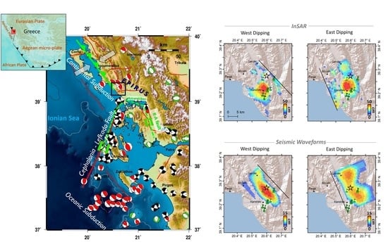
There is a spatial correlation of the estimated main slip patches with the locations of the observed landslides. Both fault dip directions explain their relative location.
The Kanallaki village, where the major damage was observed, is close or exactly above the main slip patch in all the presented models.
The InSAR and seismic waveform slip distributions agree as to the slip pattern: A west dipping fault plane would have slipped in a single main patch, whereas an east-dipping fault would have expressed two main slip patches.
The Cephalonia–Lefkada fault (which is one branch of the triple junction of western Greece—Figure 1) is known to have originated major earthquakes that consisted of double or even triple sub-events [53]. The source time function of the Kanallaki 2020 mainshock, as reported by IPGP (http://scardec.projects.sismo.ipgp.fr/ (accessed on 9 October 2020)) [54], depicts two moment release episodes. Thus, it is possible that the Kanallaki mainshock was a double-source earthquake, which could mean the existence of two main asperities like those presented in our east-dipping models.
Moreover, this means that multiple-source events are plausible even at the northern branch of the triple junction of western Greece. This possible double-source indication is an interesting insight for the area of Epirus, also because the event was only of moderate size.
Even though the stress analysis was limited to the Kanallaki sequence, the orientation of the principal axes, that is, a horizontal σ1 and a nearly vertical σ3, are compatible with the activity of the lithospheric plate movements. The thrust character of the sources and the stress orientation could indicate that the Kanallaki 2020 sequence is the result of the plate collision. Moreover, it seems that the stresses expressed by the specific sequence are separate from the activity of the other parts of the triple junction, even though the area is very close to it.
Thus, our results indicate the possibility that the Kanallaki 2020 sequence has an indicative tectonic significance. At the same time, we suggest that a moderate seismic sequences should be each time considered with skepticism with regard to what extent they can be considered a reliable indicator of the regional stress pattern or of the regional tectonics. Future major seismic events are likely to shed more light regarding the complex tectonics of North-Western Greece.

Supplementary Materials

The following are available online at https://www.mdpi.com/article/10.3390/rs13091752/s1: Figure S1: Seismic stations used during the seismic waveform inversion. Table S1: RMS InSAR non-linear Inversions.

Author Contributions

Conceptualization: N.S., A.K., A.A., S.A. and S.S.; formal analysis: N.S., A.K., C.T., A.A. and S.A.; writing—original draft preparation: N.S. and A.K.; writing—review and editing: S.S., S.A., A.A., C.T., M.P. and C.B.; visualization: N.S. and A.K. All authors have read and agreed to the published version of the manuscript.

Funding

A.K. acknowledges support through the projects “SafeSchools–T1EDK-01679” and “HELPOS-MIS5002697”, co-financed by the European Union and Greek national funds. N.S. was supported by the Italian Ministry of Economic Development (MISE) under the MISE DGISSEG-INGV 2020 project contract.

Data Availability Statement

Radar satellite data are from European Space Agency (https://scihub.copernicus.eu/ (accessed on 30 April 2020)). Digital seismic waveforms were retrieved from the ORFEUS Eida-nodes, (orfeus-eu.org), and are acquired from the following regional networks: HUSN (HL, doi:10.7914/SN/HL; HT, doi:10.7914/SN/HT; HA, doi:10.7914/SN/HA; HP, doi:10.7914/SN/HP; HI, doi:10.7914/SN/HI. Catalogue data were collected from the Department of Geophysics Aristotle University of Thessaloniki, (http://geophysics.geo.auth.gr/ss/ (accessed on 30 December 2020)) and the corresponding EMSC-CSEM online services (https://www.emsc-csem.org/ (accessed on 1 November 2020)). The Global Centroid-Moment-Tensor (CMT) Project https://www.globalcmt.org/ (accessed on 23 June 2020). The GreDaSS fault database is available at http://gredass.unife.it/ (accessed on 5 January 2021). The source time functions, IPGP (http://scardec.projects.sismo.ipgp.fr/ (accessed on 9 October 2020)).

Conflicts of Interest

The authors declare no conflict of interest. The funders had no role in the design of the study; in the collection, analyses, or interpretation of data; in the writing of the manuscript; or in the decision to publish the results.

References

  1. Valkaniotis, S.; Briole, P.; Ganas, A.; Elias, P.; Kapetanidis, V.; Tsironi, V.; Fokaefs, A.; Partheniou, H.; Paschos, P. The Mw = 5.6 Kanallaki Earthquake of 21 March 2020 in West Epirus, Greece: Reverse Fault Model from InSAR Data and Seismotectonic Implications for Apulia-Eurasia Collision. Geosciences 2020, 10, 454. [Google Scholar] [CrossRef]
  2. Lekkas, E.; Mavroulis, S.; Carydis, P.; Skourtsos, E.; Kaviris, G.; Paschos, P.; Ganas, A.; Kazantzidou-Firtinidou, D.; Parcharidis, I.; Gatsios, T.; et al. The 21 March 2020, Mw 5.7 Epirus (Greece) Earthquake. Newsl. Environ. Disaster Crises Manag. Strateg. 2020, 17, 2653–9454. [Google Scholar]
  3. Ntokos, D. Neotectonic study of Northwestern Greece. J. Maps 2018, 14, 178–188. [Google Scholar] [CrossRef] [Green Version]
  4. King, G.C.P.; Tselentis, A.; Gomberg, J.; Molnar, P.; Roecker, S.W.; Sinvhal, H.; Soufleris, C.; Stock, J.M. Microearthquake seismicity and active tectonics of the northwestern Greece. Earth Planet. Sci. Lett. 1983, 66, 279–288. [Google Scholar] [CrossRef]
  5. Hatzfeld, D.; Kassaras, I.; Panagiotopoulos, D.; Amorese, D.; Makropoulos, K.; Karakaisis, G.; Coutant, O. Microseimicity and strain pattern in northwestern Greece. TECTONICS 1995, 14, 773–785. [Google Scholar] [CrossRef]
  6. Kiratzi, A.A.; Papadimitriou, E.E.; Papazachos, B.C. Microearthquake survey in the Steno dam site in northwestern Greece. Ann. Geophys. 1987, 5, 161–166. [Google Scholar]
  7. IGRS–IFP (Institut de Géologie et Recherches du Sous-Sol, Athènes–Institut Français du Pétrole). Etude Géologique de l’Epire (Grèce Nord-occidentale); Editions Technip: Paris, France, 1966; p. 306. [Google Scholar]
  8. Makris, J. Geophysics and geodynamic implications for the evolution of the Hellenides. In Geological Evolution of the Mediterranean Basin; Stanley, J.D., Wezel, F.C., Eds.; Springer: Berlin/Heidelberg, Germany, 1985; pp. 231–248. [Google Scholar]
  9. Tselentis, A.; Sokos, E.; Martakis, N.; Serpetsidaki, A. Seismicity and Seismotectonics in Epirus, Western Greece: Results from a Microearthquake Survey. Bull. Seismol. Soc. Am. 2006, 96, 1706–1717. [Google Scholar] [CrossRef] [Green Version]
  10. Kiratzi, A. Mechanisms of Earthquakes in Aegean. In Encyclopedia of Earthquake Engineering; Beer, M., Kougioumtzoglou, I.A., Patelli, E., Siu-Kui Au, I., Eds.; Springer: Berlin/Heidelberg, Germany, 2015; pp. 1–22. [Google Scholar]
  11. Haddad, A.; Ganas, A.; Kassaras, I.; Lupi, M. Seismicity and geodynamics of western Peloponnese and central Ionian Islands: Insights from a local seismic deployment. Tectonophysics 2020, 778, 228353. [Google Scholar] [CrossRef]
  12. Pérouse, E.; Sébrier, M.; Braucher, R.; Chamot-Rooke, N.; Bourlès, D.; Briole, P.; Sorel, D.; Dimitrov, D.; Arsenikos, S. Transition from collision to subduction in Western Greece: The Katouna-Stamna active fault system and regional kinematics. Int. J. Earth Sci. 2017, 106, 967–989. [Google Scholar] [CrossRef] [Green Version]
  13. Kiratzi, A.; Sokos, E.; Ganas, A.; Tselentis, A.; Benetatos, C.; Roumelioti, Z.; Serpetsidaki, A.; Andriopoulos, G.; Galanis, O.; Petrou, P. The April 2007 earthquake swarm near Lake Trichonis and implications for active tectonics in western Greece. Tectonophysics 2008, 452, 51–65. [Google Scholar] [CrossRef]
  14. Scordilis, M.; Karakaisis, F.; Karacostas, G.; Panagiotopoulos, G.; Comninakis, E.; Papazachos, C. Evidence for transform faulting in the Ionian Sea: The Cephalonia Island earthquake sequence of 1983. PAGEOPH 1985, 123, 388–397. [Google Scholar] [CrossRef]
  15. Louvari, E.; Kiratzi, A.; Papazachos, B.C. The Cephalonia Transform Fault and its continuation to westernLefkada Island. Tectonophysics 1999, 308, 223–236. [Google Scholar] [CrossRef]
  16. Kostoglou, A.; Karakostas, V.; Bountzis, P.; Papadimitriou, E. Τhe February–March 2019 Seismic Swarm Offshore North Lefkada Island, Greece: Microseismicity Analysis and Geodynamic Implications. Appl. Sci. 2020, 10, 4491. [Google Scholar] [CrossRef]
  17. Caputo, R.; Pavlides, S. The Greek Database of Seismogenic Sources (GreDaSS), Version 2.0.0: A Compilation of Potential Seismogenic Sources (Mw > 5.5) in the Aegean Region 2013. Available online: http://gredass.unife.it/ (accessed on 5 January 2021).
  18. King, G.; Sturdy, D.; Whitney, J. The landscape geometry and active tectonics of the northwest Greece. Geol. Soc. Am. Bull. 1993, 105, 137–161. [Google Scholar] [CrossRef]
  19. Novotný, O.; Zahradník, J.; Tselentis, G. Northwestern Turkey earthquakes and the structure inferred from surface waves observed in Western Greece. Bull. Seismol. Soc. Amer. 2001, 91, 875–879. [Google Scholar] [CrossRef]
  20. Dreger, D.S. Time-Domain Moment Tensor INVerse Code (TDMT INVC) Version 1.1., 18; Berkeley Seismological Laboratory: Barkeley, CA, USA, 2002. [Google Scholar]
  21. Dreger, D.S. TDMT INV: Time domain seismic moment tensor INVersion. In International Handbook of Earthquake and Engineering Seismology; Lee, W.H.K., Kanamori, H., Jennings, P.C., Kisslinger, C., Eds.; Academic Press: Cambridge, MA, USA, 2002; p. 1627. [Google Scholar]
  22. Dreger, D.S. Berkeley seismic moment tensor method, uncertainty analysis, and study of non-double-couple seismic events. In Moment Tensor Solutions; Amico, S.D., Ed.; Springer Natural Hazards: Berlin/Heidelberg, Germany, 2018; pp. 75–92. [Google Scholar]
  23. Dreger, D.S.; Kaverina, A. Seismic remote sensing for the earthquake source process and near-source strong shaking: A case study of the 16 October 1999 Hector Mine earthquake. Geophys. Res. Lett. 2000, 27, 1941–1944. [Google Scholar] [CrossRef]
  24. Kaverina, A.; Dreger, D.; Price, E. The Combined Inversion of Seismic and Geodetic Data for the Source Process of the 16 October 1999 M 7.1 Hector Mine, California, Earthquake. Bull. Seism. Soc. Am. 2002, 92, 1266–1280. [Google Scholar] [CrossRef] [Green Version]
  25. Vavryčuk, V. Iterative joint inversion for stress and fault orientations from focal mechanisms. Geophys. J. Int. 2014, 199, 69–77. [Google Scholar] [CrossRef]
  26. Wallace, R.E. Geometry of shearing stress and relation to faulting. J. Geol. 1951, 59, 118–130. [Google Scholar] [CrossRef]
  27. Bott, M.H.P. The mechanics of oblique slip faulting. Geol. Mag. 1959, 96, 109–117. [Google Scholar] [CrossRef]
  28. Maury, J.; Cornet, F.H.; Dorbath, L. A review of methods for determining stress fields from earthquake focal mechanisms: Application to the Sierentz 1980 seismic crisis (Upper Rhine graben). Bull. Soc. Geol. Fr. 2013, 184, 319–334. [Google Scholar] [CrossRef]
  29. Vavryčuk, V. Earthquake mechanisms and stress field. In Encyclopedia of Earthquake Engineering; Beer, M., Ed.; Springer: Berlin, Germany, 2015; pp. 728–746. [Google Scholar] [CrossRef]
  30. Michael, A.J. Determination of stress from slip data: Faults and folds. J. Geophys. Res. 1984, 89, 11517–11526. [Google Scholar]
  31. Michael, A.J. Use of focal mechanisms to determine stress: A control study. J. Geophys. Res. 1987, 92, 357–368. [Google Scholar] [CrossRef]
  32. Lund, B.; Slunga, R. Stress tensor inversion using detailed microearthquake information and stability constraints: Application to Ölfus in southwest Iceland. J. Geophys. Res. 1999, 104, 14947–14964. [Google Scholar] [CrossRef]
  33. Fojtikova, L.; Vavryčuk, V. Tectonic stress regime in the 2003–2004 and 2012–2015 earthquake swarms in the Ubaye Valley, French Alps. Pure Appl. Geophys 2018, 175, 1997–2008. [Google Scholar] [CrossRef] [Green Version]
  34. Carvalho, J.; Vieira Barros, L.; Zahradník, J. Focal mechanisms and moment magnitudes of micro-earthquakes in central Brazil by waveform inversion with quality assessment and inference of the local stress field. J. South Am. Earth Sci. 2016, 71, 333–343. [Google Scholar]
  35. Massonnet, D. Satellite radar interferometry. Sci. Am. 1997, 276, 46–53. [Google Scholar]
  36. Massonnet, D.; Feigl, K.L. Radar interferometry and its application to changes in the Earth’s surface. Rev. Geophys. 1998, 36, 441–500. [Google Scholar] [CrossRef] [Green Version]
  37. Goldstein, R.; Werner, C. Radar Interferogram filtering for geophysical applications Radar interferogram filtering for geophysical applications. Geophys. Res. Lett. 1998, 25, 4035–4038. [Google Scholar]
  38. Costantini, M. A novel phase unwrapping method based on network programming. Geosci. Remote Sens. 1998, 36, 813–821. [Google Scholar]
  39. Farr, T.G.; Kobrick, M. Shuttle radar topography mission produces a wealth of data. EOS Trans. Am. Geophys. Un. 2000, 81, 583–585. [Google Scholar] [CrossRef]
  40. Yu, C.; Penna, N.T.; Li, Z. Generation of real-time mode high resolution water vapor fields from GPS observations. J. Geophys. Res. Atmos. 2017, 122, 2008–2025. [Google Scholar] [CrossRef]
  41. Yu, C.; Li, Z.; Penna, N.T.; Crippa, P. Generic atmospheric correction model for Interferometric Synthetic Aperture Radar observations. J. Geophys. Res. Solid Earth 2018, 123. [Google Scholar] [CrossRef]
  42. Yu, C.; Li, Z.; Penna, N.T. Interferometric synthetic aperture radar atmospheric correction using a GPS-based iterative tropospheric decomposition model. Remote Sens. Environ. 2018, 204, 109–121. [Google Scholar] [CrossRef]
  43. Levenberg, K. A method for the solution of certain problems in least squares. Q. Appl. Math. 1944, 2, 164–168. [Google Scholar] [CrossRef] [Green Version]
  44. Marquardt, D. An algorithm for least-squares estimation of nonlinear parameters. SIAM J. Appl. Math. 1963, 11, 431–441. [Google Scholar] [CrossRef]
  45. Okada, Y. Surface deformation due to shear and tensile faults in a half-space. Bull. Seism. Soc. Am. 1985, 75, 1135–1154. [Google Scholar]
  46. Hunstad, I.; Chini, M.; Salvi, S.; Tolomei, C.C.; Bignami, S.; Stramondo, E.; Trasatti, A. Finite fault inversion of DInSAR coseismic displacement of the 2009 L’Aquila earthquake (central Italy). Geophys. Res. Lett. 2009, 36, 15305. [Google Scholar] [CrossRef]
  47. Atzori, S.; Tolomei, C.; Antonioli, A.; Merryman Boncori, J.P.; Bannister, S.; Trasatti, E.; Pasquali, P.; Salvi, S. The 2010–2011 Canterbury, New Zealand, seismic sequence: Multiple source analysis from InSAR data and modeling. J. Geophys. Res. 2012, 117, 08305. [Google Scholar] [CrossRef]
  48. Atzori, S.; Antonioli, A.; Tolomei, C.; Novellis, V.; De Luca, C.; Monterroso, F. InSAR full-resolution analysis of the 2017–2018 M > 6 earthquakes in Mexico. Remote Sens. Environ. 2019, 234, 111461. [Google Scholar] [CrossRef]
  49. Menke, W. Geophysical Data Analysis: Discrete Inverse Theory; Academic Press: Cambridge, MA, USA, 1989. [Google Scholar]
  50. Papazachos, B.C.; Scordilis, E.M.; Panagiotopoulos, D.G.; Papazachos, C.B.; Karakaisis, G.F. Global relations between seismic fault parameters and moment magnitude of earthquakes. Bull. Geol. Soc. Greece 2004, 36. [Google Scholar] [CrossRef] [Green Version]
  51. Kapetanidis, V.; Kassaras, I. Contemporary crustal stress of the Greek region deduced from earthquake focal mechanisms. J. Geodyn. 2019, 123, 55–82. [Google Scholar] [CrossRef]
  52. Konstantinou, K.I.; Mouslopoulou, V.; Liang, W.-T.; Heidbach, O.; Oncken, O.; Suppe, J. Present-day crustal stress field in Greece inferred from regional-scale damped inversion of earthquake focal mechanisms. J. Geophys. Res. Solid Earth 2017, 122, 506–523. [Google Scholar] [CrossRef]
  53. Sokos, E.; Zahradník, J.; Gallovič, F.; Serpetsidaki, A.; Plicka, V.; Kiratzi, A. Asperity break after 12 years: The Mw6.4 2015 Lefkada (Greece) earthquake. Geophys. Res. Lett. 2016, 43, 6137–6145. [Google Scholar] [CrossRef] [Green Version]
  54. Vallée, M.; Douet, V. A new database of source time functions (STFs) extracted from the SCARDEC method. Phys. Earth Planet. Inter. 2016, 257, 149–157. [Google Scholar] [CrossRef]
Figure 1. Simplified tectonic regime near the location of the 2020 Kanallaki sequence (black rectangle) showing the triple junction of western Greece (light green notations). K–A fault notation is the Katouna–Amfilochia fault. The green dashed-line sketch of the Cephalonia–Lefkada fault Zone is based on [16]. Focal mechanisms (beachballs) indicate the representative kinematics at each area. Faults are from the GreDaSS fault database [17]. The inset shows the study area in a broader tectonic context.
Remotesensing 13 01752 g001
Figure 2. Spatial distribution of the Kanallaki 2020 sequence (green dots) for the period March–November 2020. Beach balls are focal mechanisms of the sequence (green) alongside previous available solutions (grey) for earthquakes with Mw > 5.0. The location of the Mw~6 event of 1895 is also shown (asterisk). The Margariti thrust fault sketch is based on [1], and GRCS330 and GRCS377 faults are from the GreDaSS Fault database [17]. The inset shows the magnitude histogram of the sequence.
Remotesensing 13 01752 g002
Figure 3. InSAR Line-of-Sight (LoS) surface displacement results from both the ascending and descending acquisition geometries (YYYYMMDD). “Asc” and “Desc” stand for Ascending and Descending, respectively. The detected uplifting pattern is in accordance with the thrust component indicated by the focal mechanisms.
Remotesensing 13 01752 g003
Figure 4. InSAR non-linear inversion statistics and trade-offs for an east-dipping fault. The scattered plots are showing the potential trade-offs between the various parameters. Red points are the optimal parameters in each case. Bottom histograms are the a-posteriori probability distributions of the parameters. Bell curves are indicating the Gaussian fit.
Remotesensing 13 01752 g004
Figure 5. The same with Figure 4, but for a west-dipping fault.
Remotesensing 13 01752 g005
Figure 6. InSAR and seismic waveform slip distribution models. For both types of modelling, the west dipping geometry indicates one main slip patch, while the east dipping geometry indicates two main slip patches. The black line is the fault trace. The star denotes the mainshock. Light-green flag-marks are the locations of landslides (from [1]). The different scales of the models depend on the smoothing adopted in each configuration.
Remotesensing 13 01752 g006
Figure 7. Comparison between observed and modelled InSAR deformation results of the linear inversion, for an east-dipping geometry.
Remotesensing 13 01752 g007
Figure 8. Comparison between observed and modelled InSAR deformation results of the linear inversion, for a west-dipping geometry.
Remotesensing 13 01752 g008
Figure 9. Stress inversion analysis results based on the seismic waveform focal mechanisms of the sequence. (a) Principal stress diagram. The stresses indicate a clear thrust faulting. (b) Uncertainty of the principal stresses, (c) Mohr’s cycle diagram with the positions of the faults (blue crosses). All events, except one, are in the lower semi-circle, which represents the second optimally oriented fault with Strike/Dip/Rake = 340°/20°/118° (Table 7). (d) Shape ratio histogram.
Remotesensing 13 01752 g009
Table 1. Radar satellite data used.
SatellitePre-EventPost-EventPassΔt (Days)
Sentinel-119/03/202025/03/2020Asc6
Sentinel-113/03/202025/03/2020Asc12
Sentinel-118/03/202030/03/2020Desc12
Sentinel-113/03/202025/03/2020Desc12
Sentinel-119/03/202025/03/2020Desc6
Table 2. Moment Tensor Solutions for the March 21, 2020, mainshock reported by different agencies and the solution calculated here. The GCMT scalar seismic moment = 4.78∙1017 N m. (GCMT- Global Centroid Moment Tensor; GFZ- GeoForschungsZentrum; AUTH-Aristotle University of Thessaloniki; USGS-United States Geological Survey; UOA-University of Athens; INGV-Istituto Nazionale di Geofisica e Vulcanologia; IPGP-Institut de Physique du Globe de Paris; OCA-Observatoire de la Côte d’Azur; NOA-National Observatory of Athens).
RefOrigin Time
(UTC)
Lat
°N
Lon
°E
Depth
(km)
MwStrike
(°)
Dip
(°)
Rake
(°)
Strike
(°)
Dip
(°)
Rake
(°)
DC
%
GCMT00:49:5439.1720.55135.733739119121576986
GFZ00:49:5339.3620.61165.73183790137528992
AUTH00:49:5239.3020.6275.7336381051375378100
USGS00:49:5239.3520.56145.73175187141389397
UOA00:49:5139.3120.48145.631321801446994100
INGV00:49:5139.1620.56145.733342107131507599
IPGP00:49:5139.3520.56105.8331351001395683100
OCA00:49:5139.2920.6155.731545901354590100
NOA00:49:5139.3320.5285.53153392132578985
This work00:49:51.839.30420.62175.733737106137557897
Table 3. Moment Tensor Solutions of foreshocks and major aftershocks (this work).
Date
YYYYMMDD
Origin Time (UTC)Lat (°N)Lon (°E)Depth (km)MwStrike
(°)
Dip
(°)
Rake
(°)
Strike
(°)
Dip
(°)
Rake
(°)
DC
%
VR
%
2020020121:22:2239.16820.59144.424415411272494467
2020032021:38:3039.30420.61564.23413112512165717460
2020032100:49:5239.30420.62175.73373710613755789781
2020032304:41:0339.23020.62463.92914415191801339180
2020032415:46:1039.28120.56763.6285277212564997337
2020032509:49:4539.27920.63693.91236143133696010084
2020032522:24:4039.24220.60273.6285438011848997134
2020041300:44:4139.21620.54963.4290367912455986727
2020041305:15:1639.26420.58783.33034910210643778975
2020052821:32:3639.24320.60573.33483912612559647058
Table 4. RMS InSAR Linear Inversions for the two nodal planes examined.
IntereferogramsEast DippingWest Dipping
20200313_20200325_Se_Asc0.0070.007
20200313_20200325_Sen_Des0.0040.004
20200318_20200330_Se_Des0.0030.003
20200319_20200325_Se_Asc0.0060.007
20200319_20200325_Sen_Des0.0040.004
Table 5. InSAR source results.
Strike °Dip °Rake °Geodetic Moment (N m)Moment Magnitude
West Dipping137431096.96·1017 5.8
East Dipping337371029.44·1017 5.9
Table 6. Principal stress orientations.
Stress AxisAzimuth °Plunge °
σ122515
σ21339
σ31371
Table 7. Optimally oriented faults.
IdStrike °Dip °Rake °
11255078
234020118
Publisher’s Note: MDPI stays neutral with regard to jurisdictional claims in published maps and institutional affiliations.

