Abstract
Rangelands provide significant socioeconomic and environmental benefits to humans. However, climate variability and anthropogenic drivers can negatively impact rangeland productivity. The main goal of this study was to investigate structural and productivity changes in rangeland ecosystems in New Mexico (NM), in the southwestern United States of America during the 1984–2015 period. This goal was achieved by applying the time series segmented residual trend analysis (TSS-RESTREND) method, using datasets of the normalized difference vegetation index (NDVI) from the Global Inventory Modeling and Mapping Studies and precipitation from Parameter elevation Regressions on Independent Slopes Model (PRISM), and developing an assessment framework. The results indicated that about 17.6% and 12.8% of NM experienced a decrease and an increase in productivity, respectively. More than half of the state (55.6%) had insignificant change productivity, 10.8% was classified as indeterminant, and 3.2% was considered as agriculture. A decrease in productivity was observed in 2.2%, 4.5%, and 1.7% of NM’s grassland, shrubland, and ever green forest land cover classes, respectively. Significant decrease in productivity was observed in the northeastern and southeastern quadrants of NM while significant increase was observed in northwestern, southwestern, and a small portion of the southeastern quadrants. The timing of detected breakpoints coincided with some of NM’s drought events as indicated by the self-calibrated Palmar Drought Severity Index as their number increased since 2000s following a similar increase in drought severity. Some breakpoints were concurrent with some fire events. The combination of these two types of disturbances can partly explain the emergence of breakpoints with degradation in productivity. Using the breakpoint assessment framework developed in this study, the observed degradation based on the TSS-RESTREND showed only 55% agreement with the Rangeland Productivity Monitoring Service (RPMS) data. There was an agreement between the TSS-RESTREND and RPMS on the occurrence of significant degradation in productivity over the grasslands and shrublands within the Arizona/NM Tablelands and in the Chihuahua Desert ecoregions, respectively. This assessment of NM’s vegetation productivity is critical to support the decision-making process for rangeland management; address challenges related to the sustainability of forage supply and livestock production; conserve the biodiversity of rangelands ecosystems; and increase their resilience. Future analysis should consider the effects of rising temperatures and drought on rangeland degradation and productivity.
1. Introduction
Land degradation affects ecosystem productivity and threatens its capacity to sustain human, livestock, and wildlife population specially in dryland environments. Drylands that are susceptible to desertification occupy 39.7% (~5.2 billion ha) of the global terrestrial ecosystems (~13 billion ha) [1,2]. Of this, sever land degradation is prevalent in over 10–20% of the dryland ecosystems [1,2,3]. For these reasons, land degradation in dryland ecosystems is recognized as one of the major environmental and socioeconomic challenges that can alter ecosystem services and human wellbeing [4,5,6,7]. Thus, understanding the rate, expansion, and severity of drylands degradation has received (and will continue to receive) considerable attention, due to their pivotal role in food production and water availability for more than 2 billion people in the world [3,8,9,10,11].
The main causes of drylands degradation are principally associated with population growth, overgrazing, inappropriate land and water use practices, and climate change impacts [1,11,12]. As a result, noticeable and persistent loss of vegetation cover and biomass productivity, reduction in forage and crop production, and decline in carrying capacity of rangelands are becoming common in these ecosystem [3,13,14]. Future predictions showed that climate change impacts (i.e., increase in surface air temperature and evapotranspiration, and decrease in precipitation) are expected to worsen poverty and inequality in developing countries [15,16].
Changes in above-ground biomass in drylands on which forage production and other life securing ecosystem services depend on can be measured by the net primary production (NPP) [13,17]. Several studies used temporal changes in NPP as an indicator of land degradation [2,18,19,20]. Nevertheless, the measurements and estimation of land degradation have been characterized by arbitrary assumptions, qualitative and inconsistent judgment, unreliable and spurious estimations [7,21,22]. Several studies have been criticized for underestimating the extent and severity of rangeland degradation [3,8,23]. The main reasons being the climate of dryland ecosystems (i.e., low annual precipitation and its increased interannual variability) [19,24], the successive occurrence of degradation for many decades at regional or continental scales [20], and the lack of objective measurements that quantify the extent and severity of all forms of degradation [4]. These reasons further complicate the identification of changes in dryland productivity either due to human activities (grazing and cropping) or natural variability [13,17]. Hence, the assessment of drylands degradation requires techniques that encompass spatial and temporal properties that strongly adhere to the measurement principles of repetitiveness, objectivity, and consistency [21,25]. In this regard, earth observations (OE) proved to be the only feasible means for long time and large-scale monitoring of vegetation productivity [8,9,18,24].
Vegetation indices (VIs) such as the normalized difference vegetation index (NDVI) have been used as proxy to detect and quantify long-term land degradation in drylands [6,7,11,17,18,21,25]. Two main categories of methodology have been employed to assess land degradation in drylands [7,22]—the first one observes changes in relationships between climate variables (i.e., precipitation and temperature) and VIs (i.e., measure of vegetation greenness and productivity) [8,22,23]. The second category analyzes vegetation phenology to detect structural change caused by processes such as deforestation and long-term trends [22,24]. Within each category, various methods have been applied. For example, the methods in the first category aim to control the influence of precipitation and/or temperature trends to detect permanent degradation [7,23]. The rain use efficiency (RUE) as proposed by [19]—the ratio of NPP to rainfall—has been used as an indicator of degradation [7,17,20,26,27] and ecosystem functioning [18,28]. The residual trend analysis (RESTREND) method as proposed by [11] was used frequently to estimate changes in productivity by relating annual maximum NDVI and precipitation [11,13,25,29]. In the second category, the breaks for additive and seasonal and trend (BFAST) developed by [30,31], have been employed to assess change in vegetation phenology with time (e.g., [32]).
Both RESTREND and BFAST, however, have limitations in accurately detecting land degradation when the relationship between vegetation and climate breaks and due to over sensitiveness in areas where natural climate variabilities are prevalent, respectively [5,8,22]. Over sensitiveness is represented by the detection of false breakpoints using BFAST when dryland vegetation skips phonological cycles in response to drought while the ecosystem is healthy. The time series segmented residual trend analysis (TSS-RESTREND) method was developed by [8,22,23] to address this limitation by combining BFAST and RESTREND to detect the breakpoints where the relationship between vegetation and precipitation or temperature changes [8,23]. The TSS-RESTREND leverages the ability of BFAST in detecting breakpoints in NDVI long timeseries [5,8]. The TSS-RESTREND was applied to detect land degradation in Australia and its results were qualitatively evaluated using wildfire data [8]. However, the TSS-RESTREND lacked in providing a quantitative assessment of detected breakpoints [8].
About 40% of the United States of America (USA) land is classified as drylands [33]. The largest portion of these drylands is rangelands—comprising 31% of the USA land [34]—which are mostly situated in the Western USA [35]. Rangelands support livestock production particularly beef cattle and major local economies in the Great Plains, the Intermountain West, and the Southwest rely heavily on this industry [36]. Since the pre-settlement era, about 34% of the USA rangelands have been permanently modified by human activities [37]. Woody plants encroachment, invasive species, prolonged drought, low resilience and management of rangelands could be the most critical factors that can affect current and future rangeland productivity [37,38]. Further, urban development, energy extraction (i.e., oil and gas), and expansion in agricultural lands are expected to contribute to rangelands fragmentation [39]. The degree to which climate variables (e.g., interannual variability of precipitation) can cause structural changes and affect forage productivity in New Mexico’s (NM) rangeland ecosystems has not been adequately studied. Structural change in an ecosystems can be described as the significant change in the pattern of organization of the ecosystem necessary for functioning [35]. A structural change of rangeland was considered as when a pixel has a significant break in its vegetation- precipitation relationships (VPR) that leads to irreversible degradation or significant increase in productivity. Moreover, quantitative assessment of rangeland degradation and its impacts on NM’s food-water-energy systems is critical for the sustainable use of its resources.
The goal of this study was to identify long-term structural and productivity changes in rangeland ecosystems due to interannual climate variability based on precipitation in New Mexico during the 1982–2015 period. Taking advantage of the consistent NDVI timeseries of Global Inventory Modeling and Mapping Studies (GIMMS), the study tested the hypothesis that there is no significant change in rangeland productivity in NM between 1982–2015 by evaluating the prevalence of significant difference in NM’s rangelands mean productivity before and after the years where the VPR breaks were occurred. The specific objectives were to: (1) characterize changes in rangeland productivity in terms of (a) direction of, and (b) type of structural changes in NPP as represented by NDVI using TSS-RESTREND; (2) develop an assessment framework for the identified changes in productivity; (3) use the assessment framework along with independent productivity data to identify areas affected by significant structural changes in NM’s rangeland ecosystems.
2. Data
2.1. Study Area
The study area was the state of New Mexico, USA, which covers a total land area of 314,918 km2 (Figure 1). NM’s climate is dominated by arid and semi-arid conditions with an average annual precipitation ranging from less than 254 mm in the southern desert to more than 500 mm in higher elevations in the northern part of the state [40]. The mean annual air temperature ranges from less than 4.4 °C in high mountains and valleys in the northern to 18 °C in the southern parts of the state.
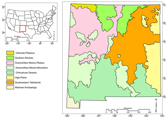
Figure 1.
A map showing the location of the New Mexico, the contiguous USA (red polygon), and the nine ecoregions within New Mexico [41].
NM’s land cover encompasses nine ecoregions that include the Chihuahua Deserts (22%) in south, southwestern part of NM, Southwestern Tablelands (22%) and Western High Plains (10%) in central, West and in the northwest parts of NM, Arizona/New Mexico Mountains (14%), Arizona/New Mexico Plateau (19%), Madrean Archipelago and southern Rockies [41] (Figure 1). Three major types of vegetation biomes (i.e., forest, shrubland and grassland) comprise the respective ecoregions [42].
2.2. Vegetation Cover
NM’s grassland biomes, particularly in the Desert Grassland Association—desert plain grassland and mixed grassland or mixed prairie—are dominated by black grama grass (Bouteloua eriopoda) and tobosa grass (Hilaria mutica) in the desert plains. Bluestem (Andropogon scoparius), san blue stem (A. halli), and Indian Grass (Sorghastrum nutans) are parts of mixed grassland or mixed prairie. Woodland biome can be found within a range of 1371 m to 2286 m elevation (amsl) and consists of one-seed juniper (Juniperus monosperma) and pinon pine (Pinus edulis) sometimes with oak (Quercus spp.) with an understory of grassland, forbs, and shrubs. Coniferous forest biomes can be found within a range of 2590 to 3658 m amsl in Petran subalpine and petran montane dominated by Enngelman spruce (Picea engel- mannii) and subalpine fir (Abies lasiocarpa). Petran montane forest association (2591.8 to 2896 m a.m.s.l) covers an extensive area of the state dominated Douglas fir, and white fir species. The land use/land cover data used in this analysis included the National Land Cover Dataset of 2011 [43] as well as the state’s ecoregions [41] and quadrants. These datasets were overlayed with the identified breakpoints to be related to changes in productivity over these different land cover types.
2.3. GIMMS NDVI
To study temporal changes in rangelands’ structure (i.e., significant changes in NPP trend), long-term NDVI timeseries was used as a proxy to NPP. Specifically, the GIMMS NDVI product based on the third generation Global Inventory Modeling and Mapping Studies NDVI (GIMM NDVIv3.1g) data was used in this study. These data was based on the Advanced Very High Resolution Radiometer (AVHRR) sensors [5,8] and it is of the most accurate datasets currently available. This version of the data corrected for calibration errors in a previous one [22]. The GIMMS NDVI data is available for the 1981–2015 period only at spatial and temporal resolutions of 8 km and 16 days, respectively. The GIMMS NDVI dataset was obtained from ECOCAST [44].
2.4. Rangeland Productivity
Rangeland productivity for the USA was obtained from the Rangeland Production Monitoring Service (RPMS) dataset developed by the United State Forest Service [45]. The dataset was prepared using NDVI from the Thematic Mapper for the 1984–2020 period at 250-meter pixels. The dataset provides estimates of annual production of rangeland vegetation in pounds per acre, which is useful in understanding trends and variability of rangeland forage resources [45]. The RPMS dataset was coupled with the assessment framework (Section 3.2) to evaluate the significance of rangeland productivity changes compared to those identified by the TSS-RESTREND method.
2.5. Precipitation, Drought, and Fire
Gridded precipitation data developed by Parameter-elevation Regressions on Independent Slopes Model (PRISM) was obtained from PRISM Climate Group [46]. Monthly precipitation at ~4 km pixels was used. To evaluate the accuracy of breakpoints in terms of timing, extent, and direction of change relative to potential disturbances, historical drought and fire events were compared with the breakpoints. Mean monthly and annual self-calibrated Palmar Drought Severity Index (PDSI) was acquired from [47]. Fire data were obtained from New Mexico Resources Geographic Information System (RGIS) [48].
3. Methods
This analysis followed three main steps—data preparation, the application of TSS-RESTREND, and the development and application of an assessment framework to evaluate the detected breakpoints and changes in productivity (Figure 2). The first step involved data acquisition, projection, resampling, and extraction of pixel values of GIMMS NDVI, PRISM precipitation, and RPMS productivity. The second step (Section 3.1) involved the application of the TSS-RESTREND method to identify breakpoints in space and time, their significance, and their structural changes. The last step provided a framework (Section 3.2) to evaluate the detected breakpoints using the RPMS—an approach that was lacking in the work by [8,23].
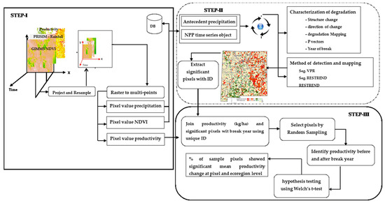
Figure 2.
Depreciation of TSS-RESTRND analysis and validation of breakpoints. In step 1, Data preparation which includes (i.e., acquisition of NPP data, precipitation, and productivity data), projection, resampling, and extraction of pixel level values. In Step II (TSS-RESTREND): method of residual fit, p-vector, trend of productivity change (i.e., decreasing, increasing, non-significance change and indeterminant), and ecosystem structure change were detected. In Step III (Evaluation), include stratified random sampling for validation, Welch’s t test on randomly selected pixels (i.e., to test the significant change of productivity before and after the break years).
3.1. Characterization of Change in Productivity Using TSS-RESTREND
3.1.1. NDVI and Precipitation Relationships
The Bimonthly GIMMS NDVI data were filtered using a quality control (QC) procedure to remove non-reliable values based on a quality flag [49,50]. Pixels with at least 75% reliable values were used. Non-vegetated pixels were excluded based on a threshold of a median NDVI of less than 0.1 [50,51]. Out of 4474 pixels, a total of 4454 pixel were used in the analysis. Complete mean monthly timeseries of NDVI (ctsNDVI) was assessed over each pixel. The PRISM precipitation data was resampled using a bilinear method to match the spatial resolution of the GIMMS NDVI and assessed at monthly time scale.
An ordinary Least Square regression (OLS) was used to develop the relationships between the ctsNDVI and the complete timeseries of optimal accumulated precipitation for each pixel for the 1982–2015 period (referred to as ctsVPR) [8]. The optimal accumulated precipitation was determined by identifying the pairs of ctsNDVI and accumulated precipitation that provide the highest correlation coefficient. The correlation coefficients of all possible OLS relationships between ctsNDVI and a matrix of precipitation accumulation period (1–12 months) with offset period (0–3 months) were evaluated following [8]. The relationships with the highest correlation coefficients were used to calculate the residual between the observed and predicted ctsNDVI (referred to as ctsVPR-residual).
3.1.2. Identification of Breakpoints
The BFAST method was applied on the ctsVPR-residual to list potential breakpoints. Briefly, the BFAST method decomposes the timeseries into season, trend, and reminder components—an approach that allows to detect changes in the season and trend components [52,53]. The list of potential breakpoints identified by the BFAST method [8] based on the ctsVPR-Residuals were further evaluated for their significance in the VPR—allowing to assess their impact on NPP as represented by the maximum NDVI timeseries. A Chow test was applied on the VPR-Residuals on all pixels with significant VPR (α = 0.05). Based on this test, all pixels that have no significant breakpoints in the VPR-Residual (α = 0.05) but have significant VPR (α = 0.05) were further assessed using the standard RESTREND by developing a regression between the VPR-Residuals and time (Equation (1)) [8].
where is intercept, is slope, and x is year
Pixels that showed significant breakpoints in VPR-Residuals (based on the Chow test above) and had significant VPR were further evaluated for the significance of these breakpoints but in the VPR also using Chow test. Pixels with significant breakpoints in VPR-Residuals but not in the VPR were further assessed using the Segmented RESTREND by developing a multivariate regression between VPR-Residual, time, and a dummy variable (Equation (2))
where is intercept, x is year, z is value of dummy variable (0 or 1), is slope, is offset at the breakpoint, and is the change in the slope at the breakpoint.
Pixels that showed significant breakpoints in VPR-Residuals and in VPR may indicate the presence of significant structural changes and thus the assumption of stationarity of the accumulation and offset periods used in the calculations of optimal accumulated precipitation before and after a breakpoint [5,54]. The set if the NDVImax and precipitation timeseries before and after a breakpoint was separated to recalculate new and independent VPR on either side of the breakpoints [8]. The precipitation data were standardized to account for the differences in the accumulation and offset periods among the breakpoints (Equation (3)).
where z is the standard score, xi is observed values, µ is the mean, and δ is the standard deviation. The NDVImax and standard score timeseries were further evaluated by fitting a multivariant regression (Equation (4)) [5,8].
where x is the standardized precipitation for year i, z the value of the dummy variable (0 or 1), β0 is intercept, β1 is slope, β2 is the offset at the breakpoint, and β3 the change in the slope at the breakpoint.
Pixels that did not meet any of the above conditions were classified as indeterminant—met the following conditions: (1) had no significant VPR and no significant breakpoints in VPR; or (2) no significant VPR, significant breakpoints in VPR, and no significant breakpoints in segmented VPR.
3.1.3. Identification of Structural Changes
Structural changes of each pixel within NM ecosystems were identified based on three properties that include the significance of the breakpoints, direction of change (i.e., increasing and decreasing in productivity), and method of detection (as described in Section 3.1.2). With the regard to the significance level and direction of change, all pixels were classified into nine categories as shown in (Table 1) following [55] and similar to other dryland degradation studies in Australia [8] and China [5].

Table 1.
Categories of threshold for vegetation change.
Consequently, a pixel can be considered having:
- Non-reversable degradation or initiation of degradation if it exhibited a breakpoint with p < 0.05 and a negative change (Table 1) in productivity as detected by Segmented VPR or Segmented RESTREND, respectively,
- Reversal or initiation of reversal in degradation, if it met the previous conditions except with a positive as detected by Segmented VPR or Segmented RESTREND, respectively,
- Stable increase in productivity, if it exhibited a breakpoint with p < 0.05 and a positive change as detected by RESTREND,
- Stable decrease in productivity if the opposite of the previous condition was detected (a condition that can be considered as an initiation of degradation) [11,13].
- Non-significant change (NSC) in productivity irrespective of the detection technique used (i.e., Segmented VPR, Segmented RESTREND, RESTREND, or Indeterminant), if it had a breakpoint with p > 0.1 and a constant direction change (i.e., 0),
- Indeterminate change if it had p = 0 and slope = 0.
A summary of the pixels based on these structural change categories was presented relative to NM’s total area, quadrant, ecoregions, and major land use/land cover classes.
3.2. Breakpoints Assessment Framework
The TSS-RESTREND method by [8] provided only a qualitative assessment of breakpoints with other independent data in terms of significance and direction of changes. These two properties are important to properly characterize changes in productivity. A framework was developed in this study to address this gap by proposed means to quantitatively assess these properties. This framework consisted of four steps: (1) Develop random samples within the identified significant breakpoints; (2) Select and use independent productivity data; (3) Evaluate the random samples at the pixel level; and (4) Group and evaluate all random samples that fall within identified ecoregions—allowing to identify whether the changes in productivity at the individual pixels are reflective of consistent regional changes.
Random Samples: A set of random samples in terms of size and location can be developed following [56,57]. To estimate the size of random samples, a prior knowledge of image accuracy/variability is required [57]. The degree of variability in the RPMS data is unknown, thus it was assumed that the maximum variability would be about 50% with 95% confidence level and ±5% precision [56]. This criterion helps to determine representative sample pixels using a stratified random sampling approach [58]. The strata were developed based on ecoregions, land use/land cover, and direction of change. Based on the formula from [57], the sample size was calculated as (Equation (5)).
where is the sample size, Z is the selected critical value of desired confidence level (1.96), p is the estimated proportion of an attribute that is present in the population (0.5), and q = 1 − p (0.5) with p and e (0.5) represent the desired level of precision.
The allocation of the random sample was based on the majority of the identified breakpoints in each method (Section 3.1.2). The random samples can be broadly allocated based on the direction of change and land cover within the identified significant breakpoints in the two main categories—the Segmented VPR and Segment RESTREND. Ecoregions and land use/land cover (NLCD 2011) [43] maps were overlaid to identify the locations of the pixels within these regions for further assessment.
Selection of independent data: The productivity data from the RPMS [45] was used to evaluate the accuracy of the identified breakpoints based on the TSS-RESTREND in terms of direction and significance of change in productivity. The data was resampled to match that of GIMMS NDVI [44,58]. Using the coordinates of GIMMS NDVI pixels, the corresponding RPMS productivity was extracted. The rangeland productivity was converted from pound per acre per year to kilogram per hectare per year. this process allowed to prepare a dataset that include RPMS productivity and with the corresponding TSS-RESTREND estimates of timing and direction of change, significance of breakpoints, and method of detection for each random sample.
Pixel level assessment: Using the location of the randomly selected samples (breakpoint pixels) and their identified year of breaks, the mean annual productivity for each pixel based on the RPMS data can be calculated for before and after the break years. Over each pixel, the number of years before and after the breaks were different and thus these mean values had different sample sizes. These mean values before and after the breaks over each pixel were then statistically compared using the Welch’s student-test for the significance in their difference and direction of change. The Welch’s t test was conducted assuming that the variances were not equal before and after the breaks [58,59]. The obtained results based on RPMS data using the Welch’s test were compared with those from the TSS-RESTREND method. A summary of the agreement of this comparison was provided over these pixels as well as over the representative land cover classes.
Ecoregion level assessment: a similar approach was followed in this step of the framework except in this case the randomly selected pixels were grouped to represent ecoregions—all sampled pixels within each ecoregion represent a single entity (analysis unit). The mean values of productivity based on RPMS of each group before their individual breaks were further averaged and compared to the corresponding average after the break. The averages were assessed for their significance and direction of change using the Welch’s student-test. The results were then compared with those obtained based on the TSS-RESTREND over the equivalent ecoregions.
4. Results
4.1. Characteristics of Change
4.1.1. Breakpoints and Direction of Change
The number of significant breakpoints detected (increased and decreased productivity) and precipitation anomalies between 1982 and 2015 were shown in Figure 3. Out of all the analyzed pixels (i.e., 4454), 814 (18.3% or ~50,000 km2) had significant breakpoints—with either increasing or decreasing trends—were detected over different land cover types. The remaining pixels that showed insignificant change (NSC), indeterminant, or identified as Agricultural represented about 55.6% (158,591 km2), 10.8% (30,656 km2) and 3.2% (9122 km2) of NM’s area (~315,900 km2). The distribution of these pixels is shown in Figure 4. Out of the 814 significant breakpoints, 52.3% (26,176 km2) and 46.5% (23,232 km2) had negative (decreasing) and positive (increasing) change in productivity, respectively (Table 2). The areas that showed significant increasing trends in productivity as I1, I2 and I3 were about 10,752 km2 (3.8%), 9408 km2 (3.3%), and 3072 km2 (1.1%) respectively. The areas that showed decreasing trend in productivity with D1, D2, and D3 level of significance were about 9088 km2 (3.2%), 13,056 km2 (4.6%), and 3776 km2 (1.3%), respectively.
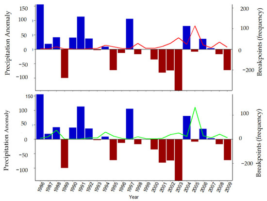
Figure 3.
A summary of the number of detected significant breakpoints along with corresponding precipitation anomaly (mm) based on a 33 year mean from PRISM. Top and bottom panels show pixels with decreasing (red line) and increasing (green line) trends in productivity, respectively.
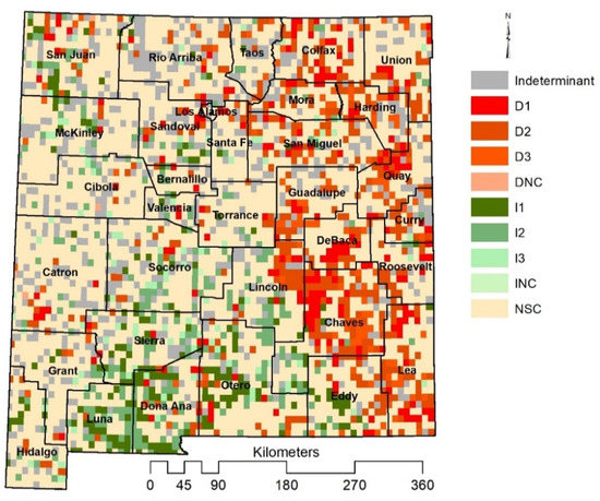
Figure 4.
The spatial distribution, significance, and direction of change in productivity using TSS-RESTREND (1982–2015). Bands of red (D1, D2, D3, D4) and green (I1, I2, I3, and INC) pixels indicate those with decreasing and increasing trends in productivity, respectively. NSC (yellow) and indeterminant (gray) pixels were those with non-significant and unidentified change, respectively.
Table 2.
A summary of the identified direction of change in productivity based on the TSS-RESTREND method in New Mexico during the 1982–2015 period.
From all significant breakpoints, 58%, 20%, and 15.7% were observed in shrubland, grassland, and evergreen forest ecosystems, respectively (Figure 5). The highest number of detected breakpoints was 250 (or 31% out of 814) in 2005. Among them, shrublands and grasslands combined accounted for 87.6% (219), out of which 72.8% and 14.8% were over shrublands and grasslands, respectively.
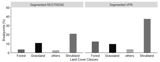
Figure 5.
The percentages of breakpoints that were identified within shrubland, grassland, evergreen forest, and other land cover types between 1982 and 2015 in NM categorized by the Segmented RESTREND and Segmented VPR methods.
4.1.2. Observed Types of Structural Changes
In general, identified breakpoints by the Segmented VPR method indicate significant ecosystem structural change—either decrease (i.e., irreversible degradation) or increase in productivity. Those identified with the Segmented RESTREND method indicate changes—either decrease (initiation of degradation) or increase (reversal from degradation)—in productivity that are not significant enough to alter the ecosystem structure.
From all obtained 814 significant breakpoints, 62.7% and 37.3% were identified using Segmented VPR and Segmented RESTREND methods, respectively. From those identified by Segmented RESTREND method, 20.8%, 10.5%, 3.4%, and 2.6% were over shrubland, grassland, evergreen forest, and other land cover classes, respectively. From those identified by Segmented VPR method, 37.3%, 12.3%, 9.5%, and 3.6% were over shrubland, evergreen forest, grassland, and other land cover classes, respectively.
The total number of pixels identified by the different methods and their direction of change were presented in Table 3. Those showed decreased (significant or insignificant) productivity were 786 or 17.6% (46,976 km2) out of 4454. About 4.9% (~14,016 km2) were identified using the Segmented VPR method; 4.3% (~12,160 km2) were identified using the Segmented RESTREND method; and the remaining 8.5% were identified using the RESTREND method (insignificant decrease or increase in productivity).
Table 3.
A summary of the pixels (in % relative to 4454 pixels) and methods used to identify the direction of change in productivity in New Mexico during the 1982–2015 period.
From all pixels that showed increased productivity (12.8% or 570 pixels, 34,816 km2), 5.7% (16,320 km2) were identified using the Segmented VPR method (i.e., significant gradual increase), 4.6% (12,992 km2) were identified using the RESTREND method (i.e., insignificant increase), and the remaining 2.5% (7168 km2) were identified using the Segmented RESTREND method (i.e., reversal of degradation).
More than half of NM’s area (55.6%~158,592 km2) show insignificant change in productivity based on the total number of pixels that fell within the NSC category (p ≥ 0.1). The pixels identified with the RESTREND method that accounted for 25.8% (~73,472 km2), and the remaining 29% were considered indeterminate.
Regionally, non-reversible decrease in productivity (i.e., degradation) was mostly observed in the northeastern (1.8%~5184 km2), northwestern (1.2%~3456 km2), and southeastern (0.99%~2816 km2) quadrants NM (Figure 6). Moreover, the initiation of degradation (i.e., decreasing trend based on the Segmented RESTREND method) was mostly detected in northeastern (1.8%~4992 km2), and southeastern (2.1%~5888 km2) quadrants, with a negligible initiation of degradation in the northwestern and southwestern NM (Figure 6).
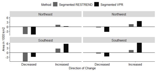
Figure 6.
Area and direction of change in productivity in northeastern, southeastern, northwestern, and southwestern quadrants of New Mexico as identified using the Segmented VPR (degraded vegetation or gradual increase) and Segmented RESTREND (reversal and initiation of degradation) methods.
From all analyzed pixels (i.e., 4454 pixels), the ones that showed increasing trends in productivity based on the Segmented VPR method (i.e., 5.7% or ~16,320 km2) were detected mostly in the southwestern (2.27%~6464 km2), southeastern (2%~5824 km2), and northwestern (1.3%~3712 km2) quadrants (Figure 6). Furthermore, 2.51% of the pixels (7168 km2) revealed reversal from degradation—increased productivity based on the Segmented RESTREND method (Figure 6). From which, 0.45% and 0.92% were in the northeastern and southeastern quadrants, respectively (Figure 6). The largest number of pixels that showed NSC was detected in northwestern (46,144 km2), while southeastern quadrant exhibited the least (32,256 km2~11.1%). Northeastern (40,896 km2) and southwestern (39,296 km2) NM revealed an equal number of NSC pixels during the study period.
4.2. Dominant Land Cover Class Changes
Significant trends (increasing or decreasing) in productivity (irreversible degradation, initiation in degradation, reversal in degradation, and initiation in reversal of degradation) were observed on NM’s dominant land cover classes that include shrubland, grassland, and evergreen forest (Figure 7).
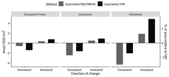
Figure 7.
Area and direction of change in productivity in grasslands, shrublands, and evergreen forests in New Mexico as identified using the Segmented VPR (degraded vegetation or gradual increase) and Segmented RESTREND (reversal and initiation of degradation) methods.
From all analyzed pixels (i.e., 4454), 2.2% of NM’s grassland (6336 km2), 4.5% of the shrubland (12,800 km2), and 1.7% of the evergreen forest pixels (4800 km2) showed significant decreasing trends in productivity–either with a complete or initiation of degradation. From all analyzed pixels, ~1.4% (3840 km2) and 0.88% (2496 km2) of NM’s grasslands that showed significant decrease in productivity were attributed to initiation of degradation (i.e., the Segmented RESTREND method) and non-reversal degradation (i.e., the Segmented VPR method), respectively (Figure 7).
Similarly, from all analyzed pixels, 2.2% (6336 km2) and 2.3% (6464 km2) of NM’s shrublands that showed significant decrease in productivity were attributed to initiation of degradation and non-reversal degradation, respectively. The degradation of shrublands was dominant in the northwestern (2048 km2) and southeastern (2112 km2) quadrants, while the degradation in grasslands was notably observed in northwestern (512 km2) and northeastern (1664 km2) quadrants.
On the other hand, 5.7% (out of the 4454 pixels) of NM’s shrubland pixels (16,248 km2), 1.3% of the grassland pixels (3648 km2), and 0.92% of the evergreen forest pixels (2624 km2) experienced either significant gradual increase in productivity or reversal of degradation (Figure 8). From all analyzed pixels, 1600 km2 (0.56%) and 2048 km2 (0.72%) of the grasslands that showed significant increase in productivity were attributed to reversal in degradation (using the Segmented RESTREND method) and significant increase in productivity (using the Segmented VPR method), respectively.
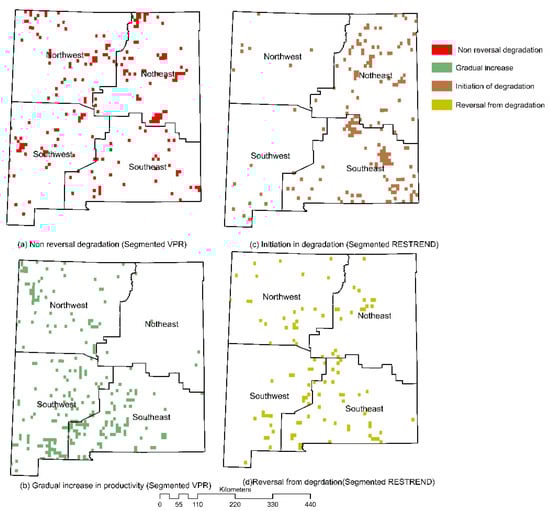
Figure 8.
Direction of change in productivity in New Mexico’s quadrants during the 1982–2015 period indicating (a) non reversal degradation, (b) gradual increase, (c) initiation of degradation, and (d) initiation of reversal from degradation along with the corresponding methods used.
4.3. Assessment of Breakpoints
This section provides a summary of the results obtained based on the breakpoints assessment framework described in Section 3.2.
4.3.1. Identified Random Samples
The total number of breakpoints based on the Segmented RESTREND and Segmented VPR methods were about 304 and 510, respectively. From which, 384 samples were randomly selected with 165 and 219 were based on the Segmented RESTREND and Segmented VPR methods, respectively (Table A1 and Table A2 in Appendix A). Since the Segmented VPR had more significant breakpoints with a noticeable change in productivity, only those pixels were subjected to the random selection. Only 155 samples out of the 219 (or 71%) showed significant difference in productivity before and after the break years (either decreasing or increasing) (Figure 9). The remaining 64 samples did not meet the criteria for significance and were not considered. From the 155 samples, 24% and 76% were obtained over grasslands and shrublands, respectively. The distribution of the grassland samples (i.e., 24%) represented the Southwestern (SW) Tablelands (46%), Arizona/New Mexico (AZ/NM) Plateau (35%), and Chihuahua Desert (16%) ecoregions. Similarly, 58%, 25%, and 11% of the shrubland samples (i.e., 76%) represented the Chihuahua Desert, AZ/NM Plateau, and SW Tablelands ecoregions, respectively.
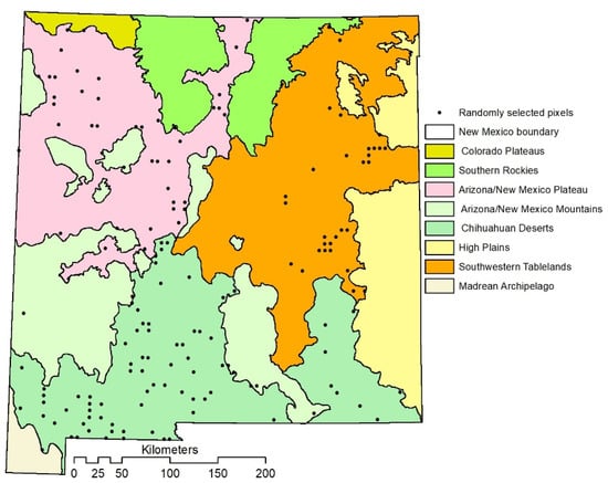
Figure 9.
The distribution of the randomly selected samples from the identified breakpoints based on the Segmented VPR method along with the ecoregions in New Mexico.
4.3.2. Changes in Productivity at Pixel Level
A summary of the comparison of the significance of the differences in mean productivity before and after the breakpoints between the Segmented VPR and the RPMS data was shown in Table 4 along with the direction (increase or decrease) of change in productivity. The results were presented as the percent of pixels that fell within each category relative to the number of the random samples (i.e., 155).
Table 4.
The percentages of pixels with decreasing and increasing trends in productivity as estimated from the RPMS data relative to randomly selected pixels (155) based on the Segmented VPR method categorized based on their significance of difference in mean productivity before and after the break years over major ecoregions in New Mexico.
Based on the Segmented VPR method, all the 155 randomly selected samples indicated significant difference in productivity before and after the break years. However, based on the RPMS only 55% of them showed significant differences in mean productivity before and after the break years until 2019, respectively (Table 4). From the 155 samples, 37% and 18% showed persistent decreasing and increasing in mean productivity after the break years until 2019 on RPMS data, respectively. About 36% and 9% showed increasing and decreasing trends before and after the break years on the RPMS data, respectively.
From the 37% of the sampled pixels that exhibited persistent decrease in mean productivity after the break years, 13% were in the Chihuahua Desert, and 18% in the SW Tablelands ecoregions. From the 18% of the sampled pixels that exhibited significant and consistent increase in mean productivity after break years, AZ/NM Mountains and AZ/NM Plateau ecoregions accounted for 3% and 15%, respectively. From the 36% of the sampled pixels with increased but insignificant difference in mean productivity before and after the break years, 35% were over the Chihuahua Desert ecoregion, and the remaining were equally obtained over AZ/NM Mountains and AZ/NM Plateau (Table 4). From the 9% of the sampled pixels with decreasing trend but insignificant difference in productivity before and after the break years, 5% were over AZ/NM Plateau.
In the sampled grasslands and shrublands pixels (i.e., 24% and 76% of the 155 samples, respectively) with either decreased or increased productivity, the difference in mean productivity before and after the break years was insignificant in 5% and 40%, respectively on RPMS (Table A3 in Appendix B). The grassland (12% of the samples) and shrubland pixels (26% of the samples) with decreased productivity had significant lower mean productivity before the break years on RPMS data. Similarly, out of the pixels that showed increased trend on productivity, 7% from grasslands and 11% from shrublands had significantly higher mean production than that before the break years on RPMS (Table A3).
4.3.3. Changes in Productivity at Ecoregion Level
A summary of the comparison between the Segmented VPR and RPMS at the ecoregion level (Section 3.2) including grassland and shrubland cover classes based on the sampled pixels (i.e., 155) was provided in Table A5 (Appendix C)—allows to highlight whether the changes at the individual pixels are reflective of those at the regional level.
Based on the RPMS data, a continuous and significant decrease in shrublands’ mean productivity after the break years in the Chihuahua (Welch’s test p ≤ 0.0001) and the AZ/NM Plateau (p = 0.0397) ecoregions was observed. Similarly, significant decline in mean productivity of grasslands of the SW Tablelands (p ≤ 0.0001) and AZ/NM (p = 0.019) ecoregions were observed after break years. The shrublands within the AZ/NM Mountains and the SW Tableland ecoregions and the grassland in Chihuahua and the AZ/NM Plateau ecoregions exhibited insignificant differences in mean productivity between before and after the break years—stable ecosystem productivity during the study period.
In contrary, the sampled pixels over the shrublands in the Chihuahua Desert (p = 0.0194) and the AZ/NM (p = 0.00765). Mountain ecoregions showed significant increase in mean productivity after the break years (Table A5). There was a significant increase in mean productivity in the grasslands within AZ/NM Plateau ecoregions after the break years. However, sampled shrubland and grassland pixels in the AZ/NM Plateau and the Chihuahua Desert, respectively, showed insignificant difference in mean productivity before and after the break years, suggesting a negligible increase in mean productivity after the break years during the study period.
5. Discussion
5.1. Characteristics of Change
The significance of the breakpoints as identified by the TSS-RESTREND methods can be interpreted relative to observed ecosystem structural changes [8,13]. Out of 67.9% of the pixels that met the criteria of RESTREND [13], 8.5% and 4.6% showed decreased and increased productivity, respectively. These pixels exhibited gradual change as their VPR remined consistent over time with no major ecosystem structural changes [13,60]. The behavior of the pixels that were identified by the Segmented VPR method (11.6%) experiencing irreversible degradation (4.9%) or increased productivity (5.7%) can partially be attributed to abrupt land use changes (decreeing or increasing) induced by human activities and climate variability [13,61] such as overgrazing or easing of drought conditions [62]. More than half of NM that did not experience significant change in productivity (NSC = 55.6%—Table 2) was dominantly in the western part of the state. This can partially be explained by the fact that western NM is the driest region in the state. Thus, it experiences weaker interactions related to climate variability and human activities—thus minimal effects on productivity. The pixels that were identified as indeterminant (10.8%) were those that none of the methods was able to fit their observed behavior [8,55] and there was no clear explanation for such behavior.
There were relatively higher human activities in northeastern, northwestern and southeastern NM represented by crude oil and natural gas production and livestock grazing practices. The prevalence of irreversible degradation and initiation of degradation were apparent in these regions [63]. On the other hand, significant changes in productivity (i.e., increase) was observed mostly in southwestern and northwestern NM, where forest were minimally influenced by human activities. On landscapes where human activities were dominant, i.e., southeastern NM, significant increase in productivity can be associated with parallel restoration activities and land use management practices [55,64].
Overall, there was a consistent increase in the number of detected significant breakpoints during the 1980s, 1990s, and 2000s, with 9.5%, 19.2%, and 71.4%, respectively (Figure 10). Again, the combined effects of climate change and anthropogenic factors can explain this increase [65]. For example, NM’s precipitation remained close to the long-term average (only recently showed increased variability) since 1920 while air temperature showed an increasing trend since 1970s [63,66,67] with a simultaneous increase in fossil fuel production activities since 1980s.
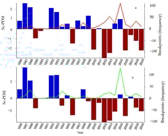
Figure 10.
A summary of breakpoints with (a) decreasing and (b) increasing trends in productivity along with the weighted average of self-calibrated Palmer Severity Drought Index (sc-PSDI).
It is challenging to identify a single factor that can be considered as the direct cause of these breakpoints and ecosystem structural changes [8,68]. However, it was possible to compare these breakpoints with some observed ecosystem structural changes whether gradual (e.g., land use management and climate change) or abrupt (e.g., wildfire). Such a comparison can help in evaluating the accuracy of these breakpoints in terms of timing, distribution, and direction of change [8,53].
5.2. Land Cover Changes Relative to Drought and Wildfire
Some of the major drivers of change in NM’s dryland ecosystems were identified as climate (e.g., drought) which is influenced by increased concentration of atmospheric greenhouse gases (GHG) (e.g., CO2); wildfire; grazing practices (i.e., livestock density); and land use conversion [21,35,68] were used here to highlight their effects on the breakpoints.
5.2.1. Detected Changes Compared to Previous Studies and Current Restoration Activities
The significant decrease in grasslands and shrublands was mostly observed in northwestern, northeastern, and southeastern NM—consistent with [4] that indicated that degradation was mostly over grassland-savanna. Degradation of grasslands, in some cases, was directly linked to increased productivity of shrublands. In NM, increased productivity in shrublands was noticed southwestern deserts and plains. This increase was attributed to land cover conversion from black grama and other valuable grasses-dominated areas to bushes due to over grazing and drought [69]. The evident climate warming, expected increase interannual precipitation variability, and projected increase in aridity can further enhance the growth of shrubs (i.e., encroachments of woody plants) over grasses since the later are heavily depended on transient surface moisture [70,71]. It was also argued that increased CO2 concentration in the atmosphere can improve plant CO2 uptake and reduce water loss through plant’s stomata thus increasing the photosynthesis process and this mechanism actually favor woody vegetation over non-woody ones [72,73].
The general notion that was suggested in some studies was that encroachments of shrublands to grasslands can be considered as one stage of degradation that can threaten the integrity of the rangelands [74]. However, it was argued that, shrublands are not necessarily degraded, nor do they necessarily represent “degradation” due to their ability to support valued ecosystem services [71,75], and they also have a long-term mean annual above ground NPP—equivalent to that of grasslands [76]. In NM, there have been a number of restoration and brush management efforts undertaken to control invasive species, and retain favored shrub species [64]. This suggested that the attribution of drivers to changes in productivity in environmental studies remains challenging owing to the diversity of driving forces and limited sources of ground truth data for validation [77].
The increased productivity in grasslands that was observed in western NM can partially be attributed to local scale successful restoration efforts by the Bureau of Land Management [64]. These efforts targeted the replacement of Creosote and mesquite by healthy grasslands, and reclamation of surfaces resulted from oil and gas extraction operations. According to Powell [78], gradual improvements in range conditions (increased productivity) in southwestern NM was not only related to the results of better moisture, but also cumulative efforts on rangeland management, such as proper stocking, vastly improved grazing distribution, and brush management.
5.2.2. Breakpoints and Drought
The sc-PSDI for NM and the detected significant breakpoints with decreasing and increasing trends were shown in Figure 10. A weighted average of the sc-PDSI was calculated over the breakpoints with decreasing and decreasing trends separately to evaluate their timing against drought events. Some previous findings suggested that extended periods of drought (or relatively dry conditions) can introduce lasting negative impacts (degradation) on rangelands and other ecosystems [8,79]. Based on Figure 10, it was noticed that from all the detected breakpoints during the study period (1982–2015), 67.9% were observed only in 2000s from which 38.2% exhibited decreased trend in productivity (Figure 10a). Coincidently, these breakpoints overlapped with frequent and extended periods of drought events in NM that were also observed regionally in the southwest USA during 2000s. The impact of this regional drought had resulted in a decrease in productivity in more than 30% of the coterminous USA, out of which ~15% (equivalent to more than 41 million ha) was rangelands [37].
The increased number of breakpoints after 2000 suggested a permanent degradation or damage to ecosystems which mechanistically can occur when these ecosystems have little to no time to recover from a previous consecutive drought event. A recovery period from a drought event as defined by [79] is the return of an ecosystem to pre-drought values of GPP and can vary from immediate to multiple years depending on vegetation, climate, disturbance, and drought. It was indicated that dryland ecosystems such as those in NM, had experienced increased recovery periods that were highly sensitive to precipitation and temperature [79]. With the expected future projections of rising temperature and drier conditions, the drought recovery of dry ecosystems would even be longer. When droughts have shorter return period (or more frequent) this makes ecosystems more susceptible to drought or ecosystem degradation continues and builds up until a threshold is reached and the degradation become irreversible (or permanent), a condition that was referred to in [79] as a tipping point. This study suggested that these thresholds may have been reached as represented by the detected breakpoints. This explains, to some extent, the appearance of breakpoints compared to drought events. The timing of these breakpoints suggested the accumulation of dry conditions that impact ecosystem functions until reaching tipping points. Further analysis is needed to understand the timing or emergence of the breakpoints and drought accumulation periods and the response of ecosystems relative to vegetation type and climate.
Moreover, these recent exceptionally drought conditions in NM (during 2000–2015) also varied in spatial extent, duration, and intensity [80]. These variations may have contributed to the occurrence of 38% breakpoints with decreasing trends (i.e., initiation and irreversible degradation) in southeastern (Eddy, Lea, Chaves, and Otero counties); northeastern (Colfax, De Bacca, and San Miguel counties); and northwestern NM (San Juan county). From all pixels that experienced significant decrease in productivity, 35% were observed in De bacca, San Miguel, San Juan, and Otero counties as drought might have a profound influence in reducing vegetation productivity (e.g., plant mortality) [81,82].
On the other hand, reversal from degradation and significant increase in productivity was dominantly observed in the northwestern, southeastern, and southwestern NM (Figure 8). In NM, wetter years were observed from 1986 to the end of 1990s, followed by drier years from 1999–2003 and 2005 (Figure 10). Significant breakpoints with increase in productivity were identified during 2000s dry years in Otero, Dona Anna, Luna, San Juan and Socorro counties. About 13.5% of these breakpoints were observed in the first four of counties. This can partially be attributed to the fact that precipitation remained near the long-term mean after the drier years over these counties that resulted in reversal from degradation or significant increase in productivity, respectively (Figure 10).
5.2.3. Breakpoints and Wildfire
Wildfire generally reduces plant cover, alters habitat structures, decrease rangeland conditions, and requires much longer recovery period [83]. The significant breakpoints with decreased productivity (i.e., irreversible degradation based on Segmented VPR) that coincided with fire events are shown in Figure 11 and Figure 12. Major wildfire incidents occurred in 1989 and 1994 followed by a consistent increase in frequency each year since 2001. This increase was noticeably concurrent with drought events. The number and time of some breakpoints mostly followed these of the fire incidents. The alignment of fire incidents with breakpoints can indicate the ability of TSS-RESTREND to detect the timing of ecosystem changes as suggested by [8]. However, based on Figure 11 and Figure 12, it appeared that only a small number of breakpoints coincided with fire incidents during the study period—suggested that fire may have a limited contribution to the development of breakpoints. While, the timing of these fire incidents can partly explain the occurrence of the breakpoints, it was not rationale to state that these fire incidents were the only direct cause of the breakpoints. Other factors need to be considered to provide a rational explanation of the remaining breakpoints such as vegetation types and their response to environmental and climate disturbance (drought). The accumulation of successive dry conditions can push an ecosystem to pass a threshold of permanent damage of vegetation—ideal fire-prone conditions. Further analysis is needed to identify the causes of breakpoints relative the fire and was out of the scope of this analysis.
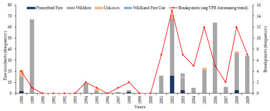
Figure 11.
Timeseries of breakpoints concurrent different types of fire incidents in New Mexico during the 1984–2015 period.
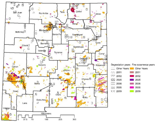
Figure 12.
A summary of breakpoints and fire incidents indicated with the timing of some major incidents.
5.3. Breakpoints and the RPMS
Based on the RPMS data, a decrease in the mean annual productivity was detected over the pixels with significant breakpoints (i.e., identified by Segmented VPR method) during the 1984–2019 period (Figure 13). The mean productivity of these pixels was lower than that of the long-term of the 36 years which was about 613.2 kg/ha. Moreover, the variability in the annual productivity of these pixels ranged from 588 kg/ha in 1995 to 641 kg/ha in 2006.
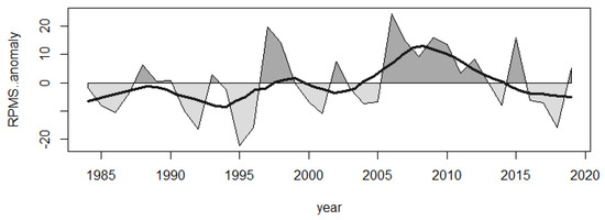
Figure 13.
Productivity anomaly based on the Range land Production Monitoring Service (RPMS) [45] averaged over the pixels that were identified with the Segmented VPR method with decreasing trend during the 1984–2019 period.
Of the sampled pixels that were evaluated for changes in productivity before and after the break years, 38% with decreasing trend showed a significant difference in mean productivity after the break years with 12% in grasslands (Table A3) and 26% in shrublands (Table A4). Similar to this finding, [84,85] indicated that there was an apparent decline in NPP in the southwestern USA that was attributed to the response of these ecosystems to the combination of a warmer temperature and a decline in precipitation. The pixels that showed significant decrease in productivity in NM’s rangeland (i.e., in Chihuahua Desert and AZ/NM plateau ecoregions) coincided with those from [45] that showed a similar behavior (Table A5). The difference in the productivity before and after the break years might be substantiated by the xeric nature of the southwestern USA and southeastern Great Plains in response to interannual variability of the precipitation [86]. On the other hand, 8% and 36% of sampled pixels with decreased and increased productivity (i.e., based on the Segmented VPR), respectively showed insignificant difference in mean productivity before and after the break years based on the RPMS data [45]. These findings were in agreement with those by [83] which suggested that the structure and composition of semi-arid and arid regions of the southwestern USA have undergone noticeable changes over the last two decades.
6. Limitation and Future Work
As the study aimed to detect degradation of vegetation, rangelands (i.e., shrubland and grasslands), the authors acknowledged some limitations that need to be considered when using these findings. The TSS-RESTREND was able to identify the breakpoints, their location, time, and type and direction of change in productivity at the state level. Due to the limited availability of ground biomass data, pixels that exhibited significant changes were validated using derived productivity from the RPMS [45] that showed only 55% agreement. Ground-based data can be more accurate means in assessing the identified breakpoints. Another important factor that can contribute to degradation is the temperature which can significantly affect NM’s dryland ecosystems.
For future, the authors would address some of these limitations using ground observations (when available) for example from the long-term rangeland monitoring observatories at the Jornada Experimental Range. The obtained breakpoints seemed consistent with some of the disturbances (drought and fire). However, the authors would consider the combined use of temperature and precipitation to improve the detection of breakpoints such as the pixels that have been classified as indeterminant. Additional quantitative analysis would be conducted to determine how drought may affect the timing of breakpoints, rangeland condition, and productivity, which can be useful in developing rangeland management practices to adapt and mitigate drought impacts.
7. Conclusions
This study evaluated the degradation of New Mexico’s rangelands during the 1984 2015 period with respect to climate using an NDVI timeseries—as a surrogate of NPP—and precipitation to represent climate variability. These datasets were evaluated using the TSS-RESTREN method to detect breakpoints in the NDVI timeseries, direction and significance of change in productivity at each pixel. The study developed a breakpoint assessment framework that allowed to quantitively evaluate the identified changes that used an independent productivity data (i.e., RPMS). A qualitative assessment of the changes against land management activities, drought, and wildfire was also conducted.
The study indicated that about 17.6% of New Mexico experienced a decrease in productivity while 12.8% of the state experienced an increase in productivity. More than half of the state (55.6%) had insignificant change productivity, 10.8% was classified as indeterminant, and the remaining 3.2% was considered as agriculture was not evaluated.
The degradation in productivity was observed in about 2.2%, 4.5%, and 1.7% of NM’s grassland, shrubland, and evergreen forest land cover classes, respectively. Simultaneously, about 5.7%, 1.3%, and 0.92% of NM’s shrublands, grasslands, and evergreen forests were characterized by an increase in productivity, respectively. Regionally, significant decrease in productivity was observed in the northeaster and southeastern quadrants of the state while significant increase was observed in northwestern, southwestern, and a small portion in southeastern quadrants. The timing and number of detected breakpoints coincided with NM’s drought frequency and severity and some fire incidents.
The TSS-RESTREN showed 55% agreement with the RPMS data over areas with significant decrease in productivity based on randomly selected pixels. Regionally, there was an agreement between the TSS-RESTREND and RPMS on the occurrence of significant degradation in productivity over the grasslands and shrublands within the Arizona/New Mexico Tablelands and in the Chihuahua Desert ecoregions, respectively.
A long timeseries assessment of rangeland productivity in New Mexico is critical to support decisions related to ecosystems management and conservation. The findings of this study can be used to address some of the rangeland degradation challenges that directly impact rangeland conditions, forage supply in the region, and New Mexican’s livelihood as these systems support livestock production. In areas where degradation was prevalent (i.e., northeastern, and southeastern NM), special intervention would be needed to conserve the biodiversity of rangeland and increase the resilience of these ecosystems. As this study considered only precipitation, it was noticed that the rising temperature can play a significant role in vegetation. Thus, future analysis should consider its effects on rangeland productivity. Future research should also pay more attention to the association of degradation and productivity with recurring droughts.
Author Contributions
Conceptualization, M.G.G. and H.M.E.G.; data curation, M.G.G. and T.A.A.; formal analysis, M.G.G.; funding acquisition, H.M.E.G.; investigation, M.G.G., H.M.E. and T.A.A.; methodology, M.G.G., H.M.E. and T.A.A.; project administration, H.M.E.G.; resources, H.M.E.G.; software, M.G.G. supervision, H.M.E.G.; validation, M.G.G., H.M.E. and T.A.A.; visualization, M.G.G., H.M.E.G. and T.A.A.; writing—original draft, M.G.G.; writing—review & editing, H.M.E.G. and T.A.A. All authors have read and agreed to the published version of the manuscript.
Funding
This research was partially funded by the National Science Foundation (NSF), awards #1739835 and#IIA-1301346, and New Mexico State University.
Data Availability Statement
The data used in this study are openly available in data [43,44,45,46,47,48].
Acknowledgments
The authors would like to thank two anonymous reviewers for their time and effort in providing valuable comments and suggestions that helped in improving the manuscript.
Conflicts of Interest
The authors declare no conflict of interest. The funders had no role in the design of the study; in the collection, analyses, or interpretation of data; in the writing of the manuscript, or in the decision to publish the results. Any opinions, findings, and conclusions or recommendations expressed in this material are those of the author(s) and do not necessarily reflect the views of the National Science Foundation.
Appendix A
Proportional allocation of the randomly sampled pixels as identified by Segmented VPR and Segmented RESTREND is shown in Table A1.
Table A1.
Allocation of the randomly selected pixels as identified with Segmented VPR method over the different land cover classes based on the National Land Cover Dataset of 2011 (NLCD 2011) along the corresponding ecoregions.
Table A1.
Allocation of the randomly selected pixels as identified with Segmented VPR method over the different land cover classes based on the National Land Cover Dataset of 2011 (NLCD 2011) along the corresponding ecoregions.
| Ecoregions | Decreasing | Increasing | NSC | Total | ||||||||
|---|---|---|---|---|---|---|---|---|---|---|---|---|
| 52 | 71 | 82 | 31 | 42 | 52 | 71 | 82 | 42 | 52 | 71 | ||
| Arizona/New Mexico Mountains | 1 | 1 | 0 | 0 | 1 | 10 | 1 | 0 | 0 | 0 | 1 | 16 |
| Arizona/New Mexico Plateau | 13 | 4 | 0 | 0 | 0 | 16 | 7 | 0 | 1 | 2 | 0 | 43 |
| Chihuahua Desert | 21 | 1 | 0 | 1 | 0 | 73 | 6 | 0 | 0 | 5 | 0 | 106 |
| Colorado Plateaus | 4 | 0 | 0 | 0 | 0 | 2 | 0 | 0 | 0 | 1 | 0 | 6 |
| High Plains | 4 | 1 | 1 | 0 | 0 | 1 | 1 | 0 | 0 | 0 | 2 | 11 |
| Madrean Archipelago | 0 | 0 | 0 | 0 | 0 | 3 | 1 | 1 | 0 | 1 | 0 | 5 |
| Southwestern Tablelands | 10 | 16 | 0 | 0 | 0 | 1 | 1 | 0 | 0 | 1 | 1 | 31 |
| Total | 53 | 24 | 1 | 1 | 1 | 106 | 18 | 1 | 1 | 9 | 4 | 219 |
31 = Bareland, 42 = Evergreen Forest, 52 = Shrub/Scrub, 71 = Grassland/Herbaceous, 82 = Cultivated Crops.
Table A2.
Allocation of the randomly selected pixels as identified with Segmented RESTREND method over the different land cover classes based on the National Land Cover Dataset of 2011 (NLCD 2011) along with the corresponding ecoregions.
Table A2.
Allocation of the randomly selected pixels as identified with Segmented RESTREND method over the different land cover classes based on the National Land Cover Dataset of 2011 (NLCD 2011) along with the corresponding ecoregions.
| Ecoregions | Decreasing | Increasing | Total | |||||||
|---|---|---|---|---|---|---|---|---|---|---|
| 22 | 52 | 71 | 90 | 95 | 42 | 52 | 71 | 52 | ||
| Arizona/New Mexico Mountains | 0 | 1 | 0 | 0 | 0 | 0 | 3 | 2 | 0 | 6 |
| Arizona/New Mexico Plateau | 0 | 1 | 2 | 1 | 0 | 0 | 6 | 4 | 0 | 13 |
| Chihuahua Desert | 1 | 37 | 1 | 0 | 1 | 0 | 25 | 4 | 0 | 68 |
| Colorado Plateaus | 0 | 1 | 0 | 0 | 0 | 0 | 1 | 0 | 0 | 1 |
| High Plains | 0 | 9 | 6 | 1 | 0 | 0 | 1 | 0 | 0 | 16 |
| Madrean Archipelago | 0 | 1 | 0 | 0 | 0 | 0 | 0 | 0 | 0 | 1 |
| Southern Rockies | 0 | 0 | 1 | 0 | 0 | 0 | 0 | 0 | 0 | 1 |
| Southwestern Tablelands | 0 | 15 | 30 | 0 | 1 | 1 | 4 | 6 | 1 | 58 |
| Total | 1 | 65 | 39 | 1 | 1 | 1 | 40 | 16 | 1 | 165 |
22 = Low Intensity Developed, 52 = Shrub/Scrub, 71 = Grassland/Herbaceous, 90 = Woody Wetlands, 95 = Emergent Herbaceous Wetlands.
Appendix B
The percentages of the randomly selected pixels (i.e., 155 identified by Segmented-VPR method) over grasslands and shrublands that were evaluated for their significance of the difference in mean productivity between before and after the break years at the pixel level using the Rangeland Production Monitoring Service (RPMS) data.
Table A3.
The percentages of the randomly selected grassland pixels with respect to their significance in the difference in mean productivity before and after the break years based on the RPMS data along with their identified direction of change over the major ecoregions in New Mexico.
Table A3.
The percentages of the randomly selected grassland pixels with respect to their significance in the difference in mean productivity before and after the break years based on the RPMS data along with their identified direction of change over the major ecoregions in New Mexico.
| Ecoregions | Insignificant Difference | Significant Difference | Total | ||
|---|---|---|---|---|---|
| Decreasing | Increasing | Decreasing | Increasing | ||
| Arizona/New Mexico Mountains | 1 | 0 | 0 | 0 | 1 |
| Arizona/New Mexico Plateau | 0 | 0 | 1 | 7 | 8 |
| Chihuahua Desert | 0 | 3 | 1 | 0 | 4 |
| Southwestern Tablelands | 1 | 0 | 10 | 0 | 11 |
| Total | 2 | 3 | 12 | 7 | 24 |
Table A4.
The percentages of the randomly selected shrublands pixels with respect to their significance in the difference in mean productivity before and after the break years based on the RPMS data along with their identified direction of change over the major ecoregions in New Mexico.
Table A4.
The percentages of the randomly selected shrublands pixels with respect to their significance in the difference in mean productivity before and after the break years based on the RPMS data along with their identified direction of change over the major ecoregions in New Mexico.
| Ecoregions | Insignificant Difference | Significant Difference | Total | ||
|---|---|---|---|---|---|
| Decreasing | Increasing | Decreasing | Increasing | ||
| Arizona/New Mexico Mountains | 1 | 1 | 0 | 3 | 5 |
| Arizona/New Mexico Plateau | 5 | 1 | 5 | 8 | 19 |
| Chihuahua Desert | 1 | 32 | 12 | 0 | 45 |
| Southwestern Tablelands | 0 | 0 | 8 | 0 | 8 |
| Total | 6 | 33 | 26 | 11 | 76 |
Appendix C
A summary of the statistical significance test result of the difference in mean in productivity before and after the break years using the randomly selected pixels (i.e., 155 identified by Segmented-VPR method) based on the Rangeland Production Monitoring Service (RPMS) data at the ecoregion level.
Table A5.
Significance of the difference in mean productivity before and after the break years based on the on increasing and decreasing shrublands and grassland randomly selected pixels using RPMS data at the ecoregion level.
Table A5.
Significance of the difference in mean productivity before and after the break years based on the on increasing and decreasing shrublands and grassland randomly selected pixels using RPMS data at the ecoregion level.
| Trend | Ecoregion | Shrublands | Grasslands | ||||
|---|---|---|---|---|---|---|---|
| Welch’s t-Statistic | df | p | Welch’s t-Statistic | df | p | ||
| Decreasing | Chihuahua Desert | −4.35 | 1379 | ≤0.0001 s | −1.23 | 39 | 0.227 |
| Arizona/New Mexico Mountains | 0.33 | 119 | 0.742 | −1.98 | 69.6 | 0.0516 | |
| Southwestern Tablelands | −1.79 | 735 | 0.0745 | −4.35 | 1053 | ≤0.0001 *** | |
| Arizona/New Mexico Plateau | 2.06 | 1122 | 0.0397 * | 2.38 | 126 | 0.019 * | |
| Increasing | Chihuahua Desert | 2.34 | 2178 | 0.0194 * | 1.47 | 196 | 0.143 |
| Arizona/New Mexico Mountains | 2.72 | 108 | 0.00765 ** | - | - | - | |
| Southwestern Tablelands | - | - | - | - | - | - | |
| Arizona/New Mexico Plateau | 1.42 | 857 | 0.157 | 2.4 | 736 | 0.065 * | |
*** p values less than or equal to 0.0001, ** p values less than 0.001, * p values less than 0.05.
References
- Katyal, J.C.; Vlek, P.L.G. Desertification: Concept, Causes and Amelioration; ZEF Discussion Papers on Development Policy, N. 33; University of Bonn, Center for Development Research (ZEF): Bonn, Germany, 2000. [Google Scholar]
- Hoover, D.L.; Bestelmeyer, B.; Grimm, N.B.; Huxman, T.E.; Reed, S.C.; Sala, O.; Seastedt, T.R.; Wilmer, H.; Ferrenberg, S. Traversing the Wasteland: A Framework for Assessing Ecological Threats to Drylands. BioScience 2020, 70, 35–47. [Google Scholar] [CrossRef]
- World Resources Institute (Ed.) Ecosystems and Human Well-Being: Desertification Synthesis: A Report of the Millennium Ecosystem Assessment; World Resources Institute: Washington, DC, USA, 2005; ISBN 978-1-56973-590-9. [Google Scholar]
- Noojipady, P.; Prince, S.D.; Rishmawi, K. Reductions in Productivity Due to Land Degradation in the Drylands of the Southwestern United States. Ecosyst. Health Sustain. 2015, 1, 1–15. [Google Scholar] [CrossRef]
- Liu, C.; Melack, J.; Tian, Y.; Huang, H.; Jiang, J.; Fu, X.; Zhang, Z. Detecting Land Degradation in Eastern China Grasslands with Time Series Segmentation and Residual Trend Analysis (TSS-RESTREND) and GIMMS NDVI3g Data. Remote Sens. 2019, 11, 1014. [Google Scholar] [CrossRef]
- Fensholt, R.; Langanke, T.; Rasmussen, K.; Reenberg, A.; Prince, S.D.; Tucker, C.; Scholes, R.J.; Le, Q.B.; Bondeau, A.; Eastman, R.; et al. Greenness in Semi-Arid Areas across the Globe 1981–2007—An Earth Observing Satellite Based Analysis of Trends and Drivers. Remote Sens. Environ. 2012, 121, 144–158. [Google Scholar] [CrossRef]
- Higginbottom, T.; Symeonakis, E. Assessing Land Degradation and Desertification Using Vegetation Index Data: Current Frameworks and Future Directions. Remote Sens. 2014, 6, 9552–9575. [Google Scholar] [CrossRef]
- Burrell, A.L.; Evans, J.P.; Liu, Y. Detecting Dryland Degradation Using Time Series Segmentation and Residual Trend Analysis (TSS-RESTREND). Remote Sens. Environ. 2017, 197, 43–57. [Google Scholar] [CrossRef]
- Gibbs, H.K.; Salmon, J.M. Mapping the World’s Degraded Lands. Appl. Geogr. 2015, 57, 12–21. [Google Scholar] [CrossRef]
- UNEP. Global Drylands: A UN System-Wide Response. Report 1. 132. Available online: https://www.unep-wcmc.org/resources-and-data/global-drylands--a-un-system-wide-response (accessed on 17 April 2021).
- Evans, J.; Geerken, R. Discrimination between Climate and Human-Induced Dryland Degradation. J. Arid Environ. 2004, 57, 535–554. [Google Scholar] [CrossRef]
- Land Degradation by Main Type of Rural Land Use in Dryland Areas. Available online: http://www.fao.org/3/X5308E/x5308e04.htm#3.%20land%20degradation%20by%20main%20type%20of%20rural%20land%20use%20in%20dryland%20areas (accessed on 14 February 2020).
- Wessels, K.J.; van den Bergh, F.; Scholes, R.J. Limits to Detectability of Land Degradation by Trend Analysis of Vegetation Index Data. Remote Sens. Environ. 2012, 125, 10–22. [Google Scholar] [CrossRef]
- Nardone, A.; Ronchi, B.; Lacetera, N.; Ranieri, M.S.; Bernabucci, U. Effects of Climate Changes on Animal Production and Sustainability of Livestock Systems. Livest. Sci. 2010, 130, 57–69. [Google Scholar] [CrossRef]
- IPBES. The Assessment Report on Land Degradation and Restoration. 748. Available online: https://www.ipbes.net/assessment-reports/ldr (accessed on 18 April 2021).
- Mirzabaev, A.J.; Wu, J.; Evans, F.; García-Oliva, I.A.G.; Hussein, M.H.; Iqbal, J.; Kimutai, T.; Knowles, F.; Meza, D.; Nedjraoui, F.; et al. Weltz, 2019: Desertification. In Climate Change and Land: An IPCC Special Report on Climate Change, Desertification, Land Degradation, Sustainable Land Management, Food Security, and Greenhouse Gas Fluxes in Terrestrial Ecosystems; Shukla, P.R., Skea, J., Buendia, E.C., Masson-Delmotte, V., Pörtner, H.-O., Roberts, D.C., Zhai, P., Slade, R., Connors, S., van Diemen, R., et al., Eds.; in press; Available online: https://www.ipcc.ch/site/assets/uploads/sites/4/2019/11/06_Chapter-3.pdf (accessed on 18 April 2021).
- Bai, Z.G.; Dent, D.L.; Olsson, L.; Schaepman, M.E. Proxy Global Assessment of Land Degradation. Soil Use Manag. 2008, 24, 223–234. [Google Scholar] [CrossRef]
- Horion, S.; Prishchepov, A.V.; Verbesselt, J.; de Beurs, K.; Tagesson, T.; Fensholt, R. Revealing Turning Points in Ecosystem Functioning over the Northern Eurasian Agricultural Frontier. Glob. Chang. Biol. 2016, 22, 2801–2817. [Google Scholar] [CrossRef] [PubMed]
- Houerou, H.N.L. Rain Use Efficiency: A Unifying Concept in Arid-Land Ecology. J. Arid Environ. 1984, 7, 213–247. [Google Scholar]
- Fensholt, R.; Rasmussen, K.; Kaspersen, P.; Huber, S.; Horion, S.; Swinnen, E. Assessing Land Degradation/Recovery in the African Sahel from Long-Term Earth Observation Based Primary Productivity and Precipitation Relationships. Remote Sens. 2013, 5, 664–686. [Google Scholar] [CrossRef]
- Andela, N.; Liu, Y.Y.; van Dijk, A.I.J.M.; de Jeu, R.A.M.; McVicar, T.R. Global Changes in Dryland Vegetation Dynamics (1988–2008) Assessed by Satellite Remote Sensing: Comparing a New Passive Microwave Vegetation Density Record with Reflective Greenness Data. Biogeosciences 2013, 10, 6657–6676. [Google Scholar] [CrossRef]
- Burrell, A.L.; Evans, J.P.; Liu, Y. The Impact of Dataset Selection on Land Degradation Assessment. ISPRS J. Photogramm. Remote Sens. 2018, 146, 22–37. [Google Scholar] [CrossRef]
- Burrell, A.L.; Evans, J.P.; Liu, Y. The Addition of Temperature to the TSS-RESTREND Methodology Significantly Improves the Detection of Dryland Degradation. IEEE J. Sel. Top. Appl. Earth Obs. Remote Sens. 2019, 12, 2342–2348. [Google Scholar] [CrossRef]
- Heumann, B.W.; Seaquist, J.W.; Eklundh, L.; Jönsson, P. AVHRR Derived Phenological Change in the Sahel and Soudan, Africa, 1982–2005. Remote Sens. Environ. 2007, 108, 385–392. [Google Scholar] [CrossRef]
- Herrmann, S.M.; Anyamba, A.; Tucker, C.J. Recent Trends in Vegetation Dynamics in the African Sahel and Their Relationship to Climate. Glob. Environ. Chang. 2005, 15, 394–404. [Google Scholar] [CrossRef]
- Prince, S.D.; Wessels, K.J.; Tucker, C.J.; Nicholson, S.E. Desertification in the Sahel: A Reinterpretation of a Reinterpretation. Glob. Chang. Biol. 2007, 13, 1308–1313. [Google Scholar] [CrossRef]
- Dardel, C.; Kergoat, L.; Hiernaux, P.; Grippa, M.; Mougin, E.; Ciais, P.; Nguyen, C.-C. Rain-Use-Efficiency: What It Tells Us about the Conflicting Sahel Greening and Sahelian Paradox. Remote Sens. 2014, 6, 3446–3474. [Google Scholar] [CrossRef]
- Bernardino, P.N.; De Keersmaecker, W.; Fensholt, R.; Verbesselt, J.; Somers, B.; Horion, S. Global-scale Characterization of Turning Points in Arid and Semi-arid Ecosystem Functioning. Glob. Ecol. Biogeogr. 2020, 29, 1230–1245. [Google Scholar] [CrossRef]
- Archer, E.R.M. Beyond the “Climate versus Grazing” Impasse: Using Remote Sensing to Investigate the Effects of Grazing System Choice on Vegetation Cover in the Eastern Karoo. J. Arid Environ. 2004, 57, 381–408. [Google Scholar] [CrossRef]
- Verbesselt, J.; Zeileis, A.; Herold, M. Near Real-Time Disturbance Detection Using Satellite Image Time Series. Remote Sens. Environ. 2012, 123, 98–108. [Google Scholar] [CrossRef]
- Verbesselt, J.; Hyndman, R.; Zeileis, A.; Culvenor, D. Phenological Change Detection While Accounting for Abrupt and Gradual Trends in Satellite Image Time Series. Remote Sens. Environ. 2010, 114, 2970–2980. [Google Scholar] [CrossRef]
- Robin, P.W.; Nackoney, J. Drylands, People, and Ecosystem Goods and Services: A Web-Based Geospatial Analysis; PDF Version; World Resources Institute; Available online: http://pdf.wri.org/drylands (accessed on 18 April 2021).
- Thomas, P.H.; Symeonakis, E. Identifying Ecosystem Function Shifts in Africa Using Breakpoint Analysis of Long-Term NDVI and RUE Data. Remote. Sens. 2020, 12, 1894. [Google Scholar] [CrossRef]
- Schuman, G.E.; Janzen, H.H.; Herrick, J.E. Soil Carbon Dynamics and Potential Carbon Sequestration by Rangelands. Environ. Pollut. 2002, 116, 391–396. [Google Scholar] [CrossRef]
- Havstad, K.; Peters, D.; Allen-Diaz, B.; Bartolome, J.; Bestelmeyer, B.; Briske, D.; Brown, J.; Brunson, M.; Herrick, J.; Huntsinger, L.; et al. The Western United States Rangelands: A Major Resource. In ASA, CSSA, and SSSA Books; Wedin, W.F., Fales, S.L., Eds.; American Society of Agronomy, Crop Science Society of America, Soil Science Society of America: Madison, WI, USA, 2015; pp. 75–93. ISBN 978-0-89118-194-1. [Google Scholar]
- Holechek, J.L.; Geli, H.M.E.; Cibils, A.F.; Sawalhah, M.N. Climate Change, Rangelands, and Sustainability of Ranching in the Western United States. Sustainability 2020, 12, 4942. [Google Scholar] [CrossRef]
- Reeves, M.C.; Mitchell, J.E. Extent of Coterminous US Rangelands: Quantifying Implications of Differing Agency Perspectives. Rangel. Ecol. Manag. 2011, 64, 585–597. [Google Scholar] [CrossRef]
- Skaggs, R.K. Ecosystem Services and Western U.S. Rangelands. Choices 2008, 23, 37–41. [Google Scholar]
- Mitchell, J.E. Rangeland Resource Trends in the United States: A Technical Document Supporting the 2000 USDA Forest Service RPA Assessment; U.S. Department of Agriculture, Forest Service, Rocky Mountain Research Station: Ft. Collins, CO, USA, 2000; p. RMRS-GTR-68.
- New Mexico Topo Maps and Outdoor Places to Visit. Available online: https://www.anyplaceamerica.com/directory/nm/ (accessed on 24 November 2019).
- Level III Ecoregions of New Mexico. Available online: https://hort.purdue.edu/newcrop/cropmap/newmexico/maps/NMeco3.html (accessed on 2 July 2020).
- Castetter, E.F. The Vegetation of New Mexico. New Mex. Q. 1956, 26, 16. [Google Scholar]
- Data|Multi-Resolution Land Characteristics (MRLC) Consortium. Available online: https://www.mrlc.gov/data (accessed on 21 September 2019).
- Ecocast Data Drop Directory. Available online: https://ecocast.arc.nasa.gov/data/pub/gimms/3g.v1/ (accessed on 5 June 2020).
- USDA. Forest Service FSGeodata Clearinghouse—Rangelands. Available online: https://data.fs.usda.gov/geodata/rastergateway/rangelands/index.php (accessed on 26 August 2020).
- PRISM Climate Group, Oregon State U. Available online: http://www.prism.oregonstate.edu/ (accessed on 29 January 2020).
- WWDT. Available online: https://wrcc.dri.edu/wwdt/time/ (accessed on 19 October 2019).
- NM RGIS|New Mexico Resource Geographic Information System Program. Available online: http://rgis.unm.edu/ (accessed on 21 September 2019).
- Quality Control Introducing the R “Gimms” Package. Available online: https://envin-marburg.gitbooks.io/introducing-the-r-gimms-package/content/chapter04/quality_control.html (accessed on 2 July 2020).
- De Jong, R.; Verbesselt, J.; Zeileis, A.; Schaepman, M. Shifts in Global Vegetation Activity Trends. Remote Sens. 2013, 5, 1117–1133. [Google Scholar] [CrossRef]
- Holben, B.N. Characteristics of Maximum-Value Composite Images from Temporal AVHRR Data. Int. J. Remote Sens. 1986, 7, 1417–1434. [Google Scholar] [CrossRef]
- Verbesselt, J.; Hyndman, R.; Newnham, G.; Culvenor, D. Detecting Trend and Seasonal Changes in Satellite Image Time Series. Remote Sens. Environ. 2010, 114, 106–115. [Google Scholar] [CrossRef]
- De Jong, R.; Verbesselt, J.; Schaepman, M.E.; de Bruin, S. Detection of breakpoints in global NDVI time series. In Proceedings of the 34th International Symposium on Remote Sensing of Environment (ISRSE), Sydney, Australia, 10–15 April 2011; Available online: https://www.zora.uzh.ch/id/eprint/77356/ (accessed on 18 April 2021).
- Fensholt, R.; Horion, S.; Tagesson, T.; Ehammer, A.; Grogan, K.; Tian, F.; Huber, S.; Verbesselt, J.; Prince, S.D.; Tucker, C.J.; et al. Assessing Drivers of Vegetation Changes in Drylands from Time Series of Earth Observation Data. In Remote Sensing Time Series; Kuenzer, C., Dech, S., Wagner, W., Eds.; Springer International Publishing: Cham, Switzerland, 2015; Volume 22, pp. 183–202. ISBN 978-3-319-15966-9. [Google Scholar]
- Li, X.B.; Li, R.H.; Li, G.Q.; Wang, H.; Li, Z.F.; Li, X.; Hou, X.Y. Human-Induced Vegetation Degradation and Response of Soil Nitrogen Storage in Typical Steppes in Inner Mongolia, China. J. Arid Environ. 2016, 124, 80–90. [Google Scholar] [CrossRef]
- PEOD5/PD005: Sampling the Evidence of Extension Program Impact. Available online: https://edis.ifas.ufl.edu/pd005 (accessed on 16 April 2021).
- Cochran, W.G. Sampling Techniques, 3rd ed.; Wiley Series in Probability and Mathematical Statistics; Wiley: New York, NY, USA, 1977; ISBN 978-0-471-16240-7. [Google Scholar]
- R: The R Project for Statistical Computing. Available online: https://www.r-project.org/ (accessed on 5 February 2020).
- Welch T-Test: Excellent Reference You Will Love—Datanovia. Available online: https://www.datanovia.com/en/lessons/types-of-t-test/unpaired-t-test/welch-t-test/ (accessed on 31 August 2020).
- Jamali, S.; Seaquist, J.; Eklundh, L.; Ardö, J. Automated Mapping of Vegetation Trends with Polynomials Using NDVI Imagery over the Sahel. Remote Sens. Environ. 2014, 141, 79–89. [Google Scholar] [CrossRef]
- Van Auken, O.W. Shrub Invasions of North American Semiarid Grasslands. Annu. Rev. Ecol. Syst. 2000, 31, 197–215. [Google Scholar] [CrossRef]
- Browning, D.M.; Maynard, J.J.; Karl, J.W.; Peters, D.C. Breaks in MODIS Time Series Portend Vegetation Change: Verification Using Long-Term Data in an Arid Grassland Ecosystem. Ecol. Appl. 2017, 27, 1677–1693. [Google Scholar] [CrossRef]
- Gedefaw, M.G.; Geli, H.M.E.; Yadav, K.; Zaied, A.J.; Finegold, Y.; Boykin, K.G. A Cloud-Based Evaluation of the National Land Cover Database to Support New Mexico’s Food–Energy–Water Systems. Remote Sens. 2020, 12, 1830. [Google Scholar] [CrossRef]
- Restore New Mexico—ScienceBase-Catalog. Available online: https://www.sciencebase.gov/catalog/item/573cda13e4b0dae0d5e4b15a (accessed on 21 January 2021).
- Loftin, S.R.; Agllilar, R.; Chung, M.C.; Alice, L.; Robbie, W.A. Desert grassland and shrubland ecosystems. In United States Department of Agriculture Forest Service General Technical Report Rm; 1995; pp. 80–94. Available online: https://www.srs.fs.usda.gov/pubs/38859 (accessed on 16 April 2021).
- Sawalhah, M.N.; Holechek, J.L.; Cibils, A.F.; Geli, H.M.E.; Zaied, A. Rangeland Livestock Production in Relation to Climate and Vegetation Trends in New Mexico. Rangel. Ecol. Manag. 2019, 72, 832–845. [Google Scholar] [CrossRef]
- Johnson, L.E.; Geli, H.M.E.; Hayes, M.J.; Smith, K.H. Building an Improved Drought Climatology Using Updated Drought Tools: A New Mexico Food-Energy-Water (FEW) Systems Focus. Front. Clim. 2020, 2. [Google Scholar] [CrossRef]
- Bond, W.J.; Midgley, G.F. Carbon Dioxide and the Uneasy Interactions of Trees and Savannah Grasses. Philos. Trans. R. Soc. B Biol. Sci. 2012, 367, 601–612. [Google Scholar] [CrossRef] [PubMed]
- Allison, R.C.D.; Ashcroft, N. New Mexico Range Plants. 48. Available online: https://aces.nmsu.edu/pubs/_circulars/CR374/ (accessed on 18 April 2021).
- Gremer, J.R.; Bradford, J.B.; Munson, S.M.; Duniway, M.C. Desert Grassland Responses to Climate and Soil Moisture Suggest Divergent Vulnerabilities across the Southwestern United States. Glob. Chang. Biol. 2015, 21, 4049–4062. [Google Scholar] [CrossRef]
- Bestelmeyer, B.T.; Peters, D.P.C.; Archer, S.R.; Browning, D.M.; Okin, G.S.; Schooley, R.L.; Webb, N.P. The Grassland–Shrubland Regime Shift in the Southwestern United States: Misconceptions and Their Implications for Management. BioScience 2018, 68, 678–690. [Google Scholar] [CrossRef]
- Ukkola, A.M.; Prentice, I.C.; Keenan, T.F.; van Dijk, A.I.J.M.; Viney, N.R.; Myneni, R.B.; Bi, J. Reduced Streamflow in Water-Stressed Climates Consistent with CO2 Effects on Vegetation. Nat. Clim. Chang. 2016, 6, 75–78. [Google Scholar] [CrossRef]
- Donohue, I.; Garcia Molinos, J. Impacts of Increased Sediment Loads on the Ecology of Lakes. Biol. Rev. 2009, 84, 517–531. [Google Scholar] [CrossRef] [PubMed]
- Mangold, J.; Monaco, T.; Sheley, R.; Sosebee, R.; Svejcar, T. Invasive Rangeland Plants. In Range and Animal Sciences and Resources Management, Vol. II; ©Encyclopedia of Life Support Systems (EOLSS), 2010; Available online: https://www.eolss.net/sample-chapters/C10/E5-35-21.pdf (accessed on 18 April 2021).
- Eldridge, D.J.; Bowker, M.A.; Maestre, F.T.; Roger, E.; Reynolds, J.F.; Whitford, W.G. Impacts of Shrub Encroachment on Ecosystem Structure and Functioning: Towards a Global Synthesis: Synthesizing Shrub Encroachment Effects. Ecol. Lett. 2011, 14, 709–722. [Google Scholar] [CrossRef]
- Peters, D.P.C. Recruitment Potential of Two Perennial Grasses with Different Growth Forms at a Semiarid-Arid Transition Zone. Am. J. Bot. 2002, 89, 1616–1623. [Google Scholar] [CrossRef]
- Cherlet, M.; Hutchinson, C.; Reynolds, J.; Hill, J.; Sommer, S.; von Maltitz, G. World Atlas of Desertification Rethinking Land Degradation and Sustainable Land Management; European Union: Luxembourg, 2018; ISBN 978-92-79-75350-3. [Google Scholar]
- Powell, J.C. Rangelands of southwest New Mexico—An upside view. Rangelands 1992, 14, 265–268. [Google Scholar]
- Schwalm, C.R.; Anderegg, W.R.; Michalak, A.M.; Fisher, J.B.; Biondi, F.; Koch, G.; Litvak, M.; Ogle, K.; Shaw, J.D.; Wolf, A. Global Patterns of Drought Recovery. Nature 2017, 548, 202–205. [Google Scholar] [CrossRef]
- Preparedness Bureau Mitigation|NM Department of Homeland Security & Emergency. Available online: https://www.nmdhsem.org (accessed on 16 April 2021).
- Lotsch, A. Response of Terrestrial Ecosystems to Recent Northern Hemispheric Drought. Geophys. Res. Lett. 2005, 32, L06705. [Google Scholar] [CrossRef]
- Ponce-Campos, G.E.; Moran, M.S.; Huete, A.; Zhang, Y.; Bresloff, C.; Huxman, T.E.; Eamus, D.; Bosch, D.D.; Buda, A.R.; Gunter, S.A.; et al. Ecosystem Resilience despite Large-Scale Altered Hydroclimatic Conditions. Nature 2013, 494, 349–352. [Google Scholar] [CrossRef] [PubMed]
- Snyman, H.A. Estimating the Short-Term Impact of Fire on Rangeland Productivity in a Semi-Arid Climate of South Africa. J. Arid Environ. 2004, 59, 685–697. [Google Scholar] [CrossRef]
- Reeves, M.C.; Baggett, L.S. A Remote Sensing Protocol for Identifying Rangelands with Degraded Productive Capacity. Ecol. Indic. 2014, 43, 172–182. [Google Scholar] [CrossRef]
- Polley, H.W.; Briske, D.D.; Morgan, J.A.; Wolter, K.; Bailey, D.W.; Brown, J.R. Climate Change and North American Rangelands: Trends, Projections, and Implications. Rangel. Ecol. Manag. 2013, 66, 493–511. [Google Scholar] [CrossRef]
- Zhao, M.; Running, S.W. Drought-Induced Reduction in Global Terrestrial Net Primary Production from 2000 Through 2009. Science 2010, 329, 940–943. [Google Scholar] [CrossRef] [PubMed]


Publisher’s Note: MDPI stays neutral with regard to jurisdictional claims in published maps and institutional affiliations. |
© 2021 by the authors. Licensee MDPI, Basel, Switzerland. This article is an open access article distributed under the terms and conditions of the Creative Commons Attribution (CC BY) license (https://creativecommons.org/licenses/by/4.0/).