Spatiotemporal Changes of Winter Wheat Planted and Harvested Areas, Photosynthesis and Grain Production in the Contiguous United States from 2008–2018

Abstract

Winter wheat is a main cereal crop grown in the United States of America (USA), and the USA is the third largest wheat exporter globally. Timely and reliable in-season forecast and year-end estimation of winter wheat grain production in the USA are needed for regional and global food security. In this study, we assessed the consistency between the agricultural statistical reports and satellite-based data for winter wheat over the contiguous US (CONUS) at both the county and national scales. First, we compared the planted area estimates from the National Agricultural Statistics Service (NASS) and the Cropland Data Layer (CDL) from 2008–2018. Second, we investigated the relationship between gross primary production (GPP) estimated by the vegetation photosynthesis model (VPM) and grain production from the NASS. Lastly, we explored the in-season utility of GPP_VPM in monitoring seasonal production. Strong spatiotemporal consistency of planted areas was found between the NASS and CDL datasets. However, in the Southern Great Plains, both the CDL and NASS planted acreage were noticeable larger (>20%) than the NASS harvested area, where some winter wheat fields were used as forage for cattle grazing. County-level GPP_VPM was linearly related with grain production of winter wheat, with an R² value of 0.68 across the CONUS. The relationships between grain production and GPP_VPM in those counties without a substantial difference (<20%) between planted and harvested area were much stronger and their harvest index (HI_GPP) values ranged from 0.2–0.3. GPP_VPM in May could explain about 70–90% of the variance of winter wheat grain production. Our findings highlight the potential of GPP_VPM in winter wheat monitoring, especially for those high harvested/planted ratio, which could provide useful data to guide planning and marketing for decision makers, stakeholders, and the public.

1. Introduction

Wheat is one of the most widely cultivated grain crops in the world, covering approximately one sixth of the total arable land area, and wheat grain contributes ~20% of total dietary calories worldwide [1]. Wheat is also widely traded in the world food market with approximately ~23% of the world’s annual wheat grain production being traded internationally. The United States of America (USA) ranks the fifth for wheat production (after the European Union, China, India, and Russia) and the third for wheat grain export (after Russia and the European Union) [2]. Winter wheat dominates the USA wheat grain production, accounting for approximately 80% of national wheat production [3]. The interannual fluctuation of winter wheat production in the USA could have significant impacts on the international wheat trade and global food security. Therefore, timely, reliable, and spatially explicit information on winter wheat planted and harvested areas, grain yield, and production are critical for regional and global food security as well as international food trade.

The agricultural surveys and statistical reports by governmental agencies have been the major data sources for crop acreages (including planted and harvested area), grain yield, and grain production for each year from county to national scales [4,5,6,7]. The U.S. Department of Agriculture (USDA) National Agricultural Statistics Service (NASS) leads the effort for in-season forecast and year-end estimation of grain production of most crops grown in the USA. Each year, the NASS conducts several surveys and extensive field observations to collect a variety of data needed to fulfill this task [6,7]. Spatially, an efficient sample design is usually required for agricultural surveys to provide crop estimates over regions. However, the sampling fields only covers part of the intended region. Temporally, it takes time for the government to gather and process the survey data and, for information confidentiality, the agricultural survey data usually have a scheduled release. There are no reports or data available between the scheduled releases. Thus, agricultural surveys are usually time consuming, expensive, and have spatial and temporal gaps [8].

Satellite-based Earth observation has been a viable technology for identifying and mapping planted and harvested crop areas since the early 1970s [9]. Numerous studies have used multiple temporal remote sensing data to characterize and map individual crop types [10,11,12,13,14]. The Cropland Data Layer (CDL) datasets, released by the NASS/USDA [15], have reported annual planted areas for all major crops in the contiguous United States (CONUS) since 2008. Annual maps of pixel-based crop planted areas from the CDL provide supplementary acreage estimates to NASS acreage survey data, but it was reported that CDL-based crop planted area estimates were slightly lower than the NASS statistical estimates [15]. To date, there has no systematic comparative study to examine the spatiotemporal consistency of winter wheat planted area estimates between NASS and CDL datasets from 2008–2018 in the CONUS. Additionally, the spatiotemporal consistency and dynamics between winter wheat planted areas (CDL, NASS) and harvested area (NASS) from 2008–2018 in the CONUS has not been investigated.

Satellite remote sensing is also widely applied in estimating crop yield or production [16,17,18,19]. The process-based mathematical models and statistical regression models use climate inputs and satellite images to predict crop yield [20,21,22,23]. Climate variables, such as downward short-wave radiation, air temperature, and precipitation, are common inputs in those models [20,24]. Though climate data describe the environmental conditions that affect crop growth, it cannot directly measure the impacts of abiotic and biotic factors on crop growth. Climate data are usually used with other datasets to predict crop yield [21]. Vegetation indices, such as the enhanced vegetation index (EVI) and normalized difference vegetation index (NDVI), are widely utilized to monitor crop growth status and estimate crop yield [22,25,26]..

Gross and net primary production (GPP, NPP, respectively), aboveground biomass (AGB), and grain production and yield (GP, GY, respectively) of crop fields are interlinked by the concept of the harvest index (HI), which can be defined in three ways: (1) HI_AGB = GY/AGB, (2) HI_NPP = GY/NPP, and (3) HI_GPP = GY/GPP. Most of the agricultural literature uses HI_AGB or HI_NPP to estimate crop yield and/or grain production [27,28,29]. GPP estimates from light use efficiency (LUE) models driven by climate and satellite data are available to the public [30,31,32]. Crop yield is estimated from GPP and GPP-based HI (HI_GPP). He et al. [26] modeled HI_GPP from county-level MODIS GPP and grain production statistics for croplands in Montana from 2008–2015 and applied the HI_GPP for yield prediction in Montana. For maize and soybean croplands in the CONUS, Wu et al. [33] reported strong relationships between GPP simulated by the vegetation photosynthesis model (VPM) and grain production from the NASS, and there are small interannual changes of HI_GPP. However, knowledge is still limited on the spatiotemporal relationship between GPP and grain production in the CONUS and on the performance of GPP for in-season grain production forecasting for winter wheat.

In this study, as one of a series of papers to explore the relationship between GPP_VPM and grain production, we followed the general framework of the previous paper [33]. However, this paper focused on winter wheat croplands. First, we investigated the spatiotemporal dynamics of winter wheat cropping areas in the CONUS at national and county scales from 2008 to 2018. We quantified the spatiotemporal consistencies between NASS and CDL datasets for planted areas and for planted/harvested areas. Differences between winter wheat planted area and harvested area were expected because winter wheat fields can be used as dual-purpose fields: beef cattle grazing and/or grain production. This is a typical phenomenon in the Southern Great Plains (SGP). Second, we hypothesize that the relationships between winter wheat GPP and grain production are strong and linear. We analyzed the spatiotemporal dynamics of winter wheat GPP and grain production over the CONUS at national and county scales from 2008–2018. The GPP data are derived from the VPM (GPP_VPM), which were evaluated with GPP data from the in situ cropland eddy flux tower sites (GPP_EC) [30]. Third, we explored the relationships between GPP_VPM and NASS grain production and quantified the ratio between GPP and grain production, namely, GPP-derived harvest index (HI_GPP). Finally, we assessed the linear regression models between county-level cumulated GPP over time and annual grain production and explored the potential to monitor winter wheat grain production in the CONUS within the growing season of winter wheat.

2. Materials and Methods

2.1. Study Area

The CONUS includes 3233 counties and 48 states. The climate is diverse, ranging from a temperate climate in the northern region to a subtropical climate in the southern region (e.g., Florida). Winter wheat is primarily cultivated in the Great Plains (Figure 1). The Southern Great Plains (Texas, Oklahoma, and Kansas) are the largest winter wheat producing region, accounting for over 40% of national wheat grain production in the USA [34]. Winter wheat cultivation is largely rain-fed. Note that in the Southern Great Plains, varying areas of winter wheat fields are used as dual-purpose fields: beef cattle grazing and/or grain production, dependent upon weather, market conditions, and other factors [35].

2.2. Winter Wheat Planted and Harvested Areas, and Grain Production Data from 2008–2018 from the USDA NASS Statistical Dataset

The USDA National Agricultural Statistic Service (NASS) Quick Stats database (https://quickstats.nass.usda.gov/, accessed on 28 April 2021) provides annual statistics on crop acreages (planted and harvested area) and grain production at national and county scales. The NASS crop statistical data are derived from the surveys of farm operators, grain processors, commercial storage firms, in situ yield samples, etc. As an example, the NASS winter wheat planted area and harvested area estimates come mostly from the Agricultural Survey in December and June. Farmers are asked by NASS survey enumerators about the acreage they planted and the acreage they plan to harvest [3]. The grain yield statistical data were derived from both the Objective Yield Survey (OYS) and Agricultural Yield Survey (AYS). The AYS is based on farmers’ reported yield and the OYS is based on crop biophysical measurements of selected samples. Grain production is calculated by yield estimates at survey dates and to-be-harvested area, and predicted by assuming normal weather conditions for the remaining part of the growing season.

2.3. Winter Wheat Planted Area Data from the USDA NASS Cropland Data Layer Dataset (CDL)

The annual CDL dataset at a 30 m spatial resolution includes more than one hundred crop types in the CONUS [15]. The CDL dataset is produced by using a machine learning method, in situ reference data, and multi-date satellite images to identify crop types. The training data used in the crop classification include the National Land Cover Dataset (NLCD) and the USDA Farm Service Agency (FSA) Common Land Unit (CLU) data. The CLU attributes include the crop types and acreages reported by producers to the FSA county offices in the early growing season. The CDL classifier utilizes multiple temporal remote sensing images from multiple sensors, including Landsat TM/ETM+, AWiFS, Deimos-1, UK-DMC-2, and MODIS images [15]. The spatial resolution of the CDL dataset is 30 m from 2010–2018 and 56 m from 2008–2009. In 2018, the CDL data for 2008 and 2009 were reprocessed to 30 m. The CDL data from 2008 to 2018 at a 30 m spatial resolution were used, which ensures the spatial resolution is consistent during the study period.

The CDL dataset provides detailed spatial information for individual crop types, and high classification accuracies (>90%) for major crop types (e.g., winter wheat, soybean, and maize) were reported [15]. Numerous agriculture-related studies and land cover change studies have used the CDL dataset [36,37,38,39]. CropScape, which is a web-based data portal, provides interactive tools for people to download, visualize, and analyze the CDL data in a more effective and efficient way [40]. The annual total planted area of winter wheat in each county was calculated from CropScape. The national total areas in each year were then calculated as the total of annual planted crop areas over all the counties in the nation.

2.4. Gross Primary Production Estimates for Winter Wheat from the Vegetation Photosynthesis Model (GPP_VPM)

The VPM estimates the daily GPP from the amount of PAR absorbed by chlorophyll (APAR_chl) and the light use efficiency [41,42]. GPP derived from the eddy-covariance tower sites (GPP_EC) was used to assess daily GPP_VPM in different croplands, including winter wheat [43,44], soybean [45,46], paddy rice [47], maize [45,48], and sugarcane [49]. Strong temporal consistency between GPP_EC and GPP_VPM was reported in the aforementioned publications, with R² values ranging from 0.70 to 0.98. The driving data of the VPM include vegetation indices (land surface water index (LSWI) and EVI) and meteorological data (air temperature, shortwave radiation). The theory, model structure, and parameters of the VPM were documented in [30,31]. We followed the same procedure to run VPM simulations as reported in an earlier publication [30], which used different maximum light use efficiency (LUE₀) parameter values for C₃ and C₄ crops to improve GPP estimation in croplands, as follows:

GPP = APAR_chl × LUE

(1)

APAR_chl = FPAR_chl × PAR

(2)

LUE = LUE₀ × T_scalar × W_scalar

(3)

LUE₀ = LUE_0-C3 × FA_C3 + LUE_0-C4 × FA_C4

(4)

where FPARchl is the fraction of PAR absorbed by chlorophyll in the canopy; LUE₀ is the maximum light use efficiency without environmental stress; Tscalar and Wscalar are the temperature and water limitation scalars; FA_C3 and FA_C4 are the area fractions of C₃ and C₄ plants within each 500 m MODIS pixel (range of 0–1.0), LUE_0-C3 and LUE_0-C4 are the maximum LUE values for C3 and C4 plants, respectively.

The growing season total GPP of winter wheat at each pixel was calculated by summarizing daily GPP between the USDA planted and harvested dates. The mean GPP values in each county during the growing season were area weighted according to the area fraction of winter wheat in a county derived from the CDL datasets within 500 m pixels. More details about the VPM and GPP calculation can be found in [33]. The growing season total GPP of winter wheat in each county was calculated by the mean GPP multiplied by the total area of winter wheat within all pixels in the county (Figure 1f).

2.5. Statistical Analysis

To explore the interannual changes of winter wheat cropping areas and grain production from 2008–2018, we calculated the anomaly of each variable as the difference between the value in a specific year and the multi-year average from 2008–2018, and then normalized it by the multi-year average. We used linear regression models to quantify the relationships between grain production and cropping areas, and between GPP_VPM and grain production at national and county scales. The performance of models was assessed using the coefficient of determination (R²), bias, and root mean square error (RMSE) between the modeled grain production estimates and the NASS grain production statistics. The regression slope between grain production and GPP_VPM, representing the conversion coefficient from GPP_VPM to grain production, was also termed as the GPP-based harvest index (HI_GPP).

$$R^2={\left(\frac{{{\displaystyle \sum }}_{i=1}^n\left(G{P}_{sim}\left(i\right)-\overline{G{P}_{sim}}\right)\times \left(\left(G{P}_{NASS}\left(i\right)-\overline{G{P}_{NASS}}\right)\right)}{\sqrt{{{\displaystyle \sum }}_{i=1}^n{\left(G{P}_{sim}\left(i\right)-\overline{GP{P}_{sim}}\right)}^2}\sqrt{{{\displaystyle \sum }}_{i=1}^n{\left(G{P}_{NASS}\left(i\right)-\overline{GP{P}_{NASS}}\right)}^2}}\right)}^2$$

(5)

$$RMSE=\sqrt{{{\displaystyle \sum }}_{i=1}^n{\left(G{P}_{sim}\left(i\right)-G{P}_{NASS}\left(i\right)\right)}^2/n}$$

(6)

$$bias=G{P}_{sim}-G{P}_{NASS}$$

(7)

where GP_sim is the simulated grain production at a county scale based on linear models, $\overline{G{P}_{sim}}$ is the mean GP_sim across counties in the CONUS, i is the county number, and n is the total number of counties. As there are missing NASS statistics data for some counties over the years, we only kept those counties with continuous data from 2008–2018. The total number is 795. GP_NASS is the NASS grain production, $\overline{G{P}_{NASS}}$ is the mean GP_NASS across counties in the CONUS.

2.6. In-Season Forecasting of Winter Wheat Grain Production Using Cumulated GPP_VPM Data

Accurate and timely prediction of grain production and yield is one requirement in crop production monitoring programs. To explore the in-season prediction skill from GPP_VPM, linear regression models were applied between cumulated GPP (GPP_cum) over time and grain production at the county scale (see Equation (1)).

$$Grain Production=a\times {{\displaystyle \sum }}_1^t(GP{P}_t\times k)+b\hspace{1em}\hspace{1em}\hspace{1em}t=1,2,3,\dots ,46$$

(8)

where t is the time intervals in a year (ranging from 1 to 46), as GPP_VPM data are at an 8-day temporal resolution and have 46 estimates within each year; k is the number of days within a time interval, being 8 days for t = 1 to 45, and 5 or 6 days (non-leap year, leap year) for t = 46. In this study, we used a calendar year schedule to run the statistical models for all counties, though winter wheat is usually planted in late fall of the previous year (e.g., late September to October). The GPP_cum in the previous fall season is usually low and was not included in Equation (1), as we tried to make the task simple, without delineating the exact planting dates of winter wheat in the fall season of the previous year. We also assumed that it has a negligible effect on the modeling skills.

3. Results

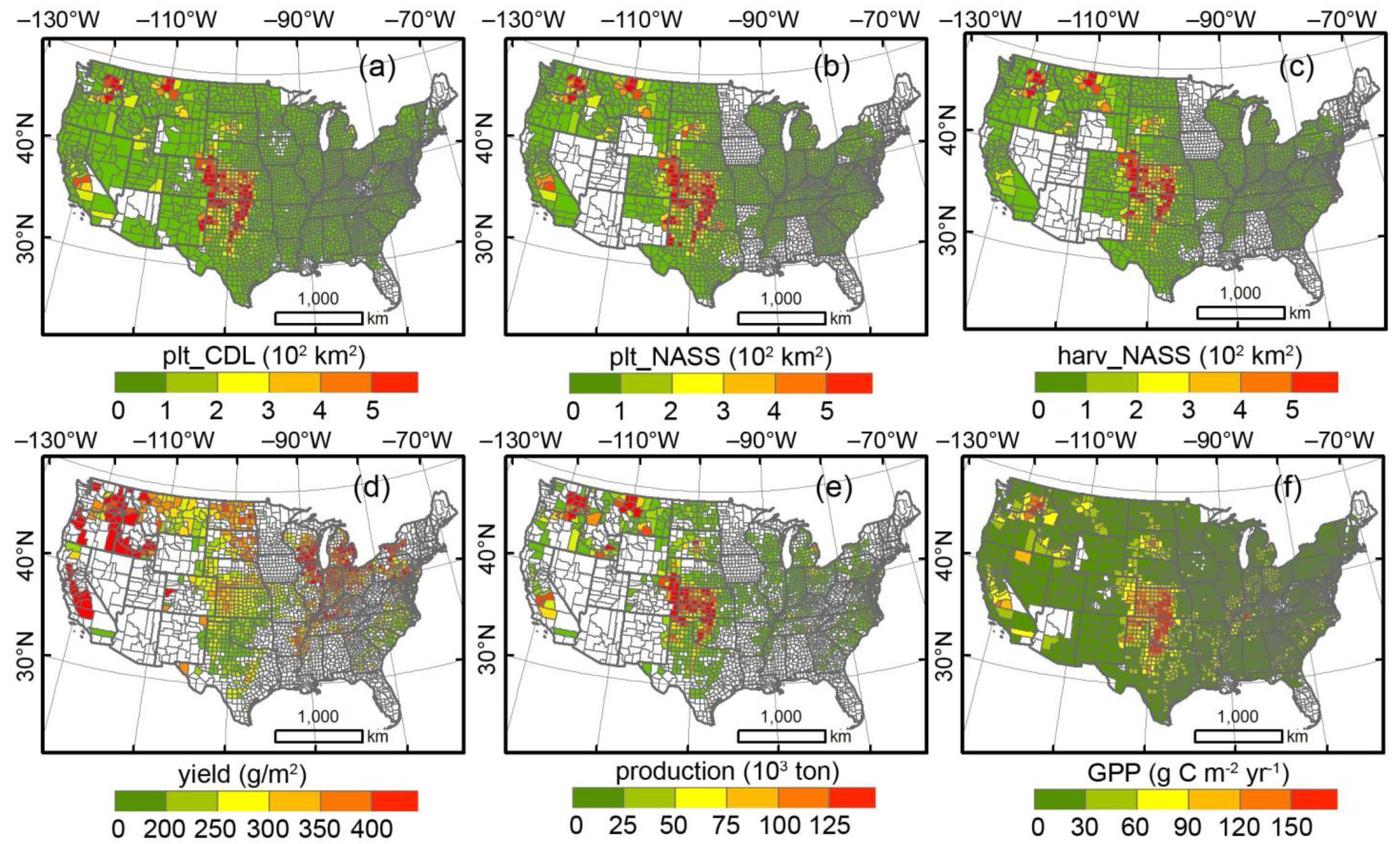
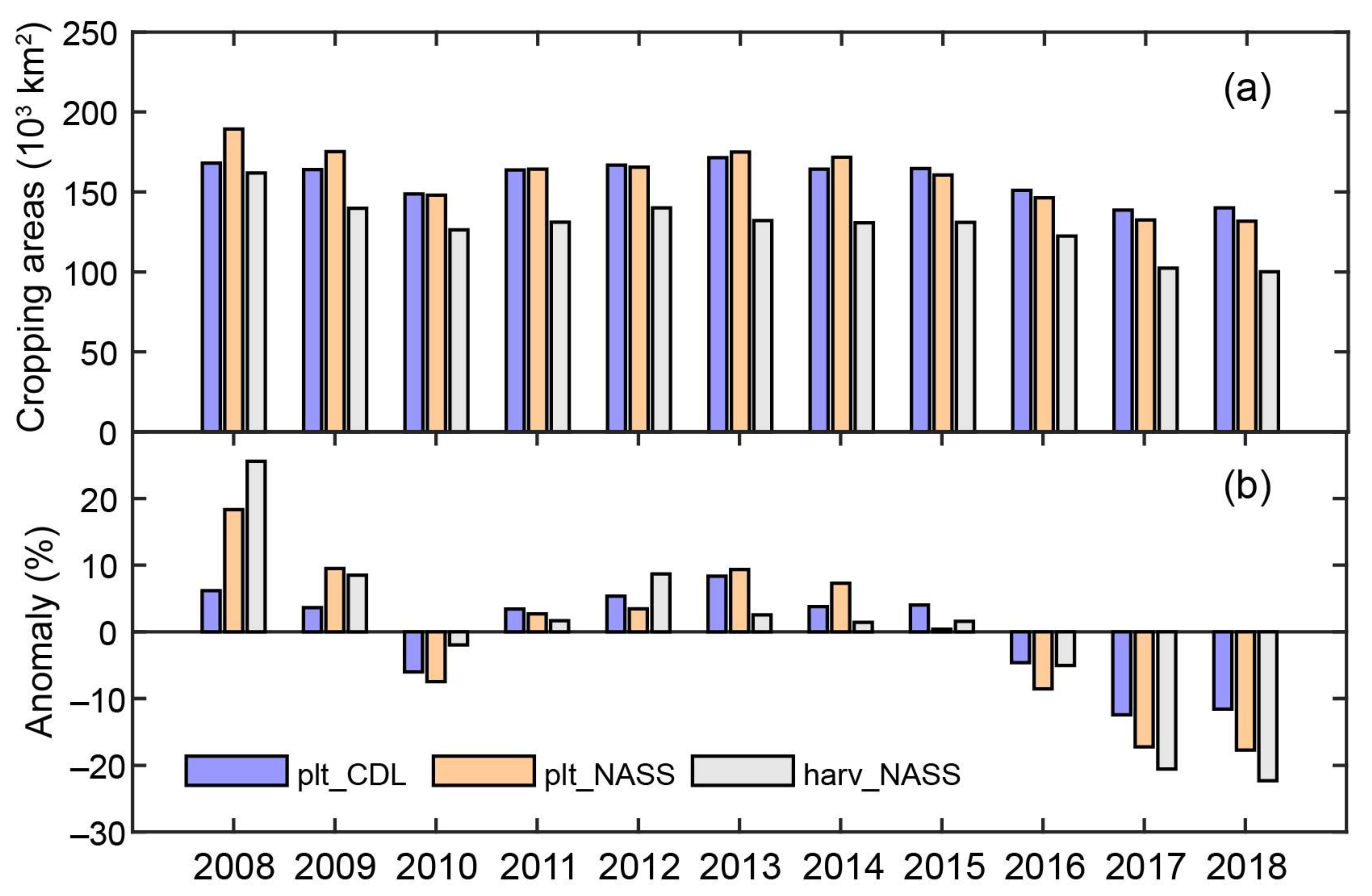
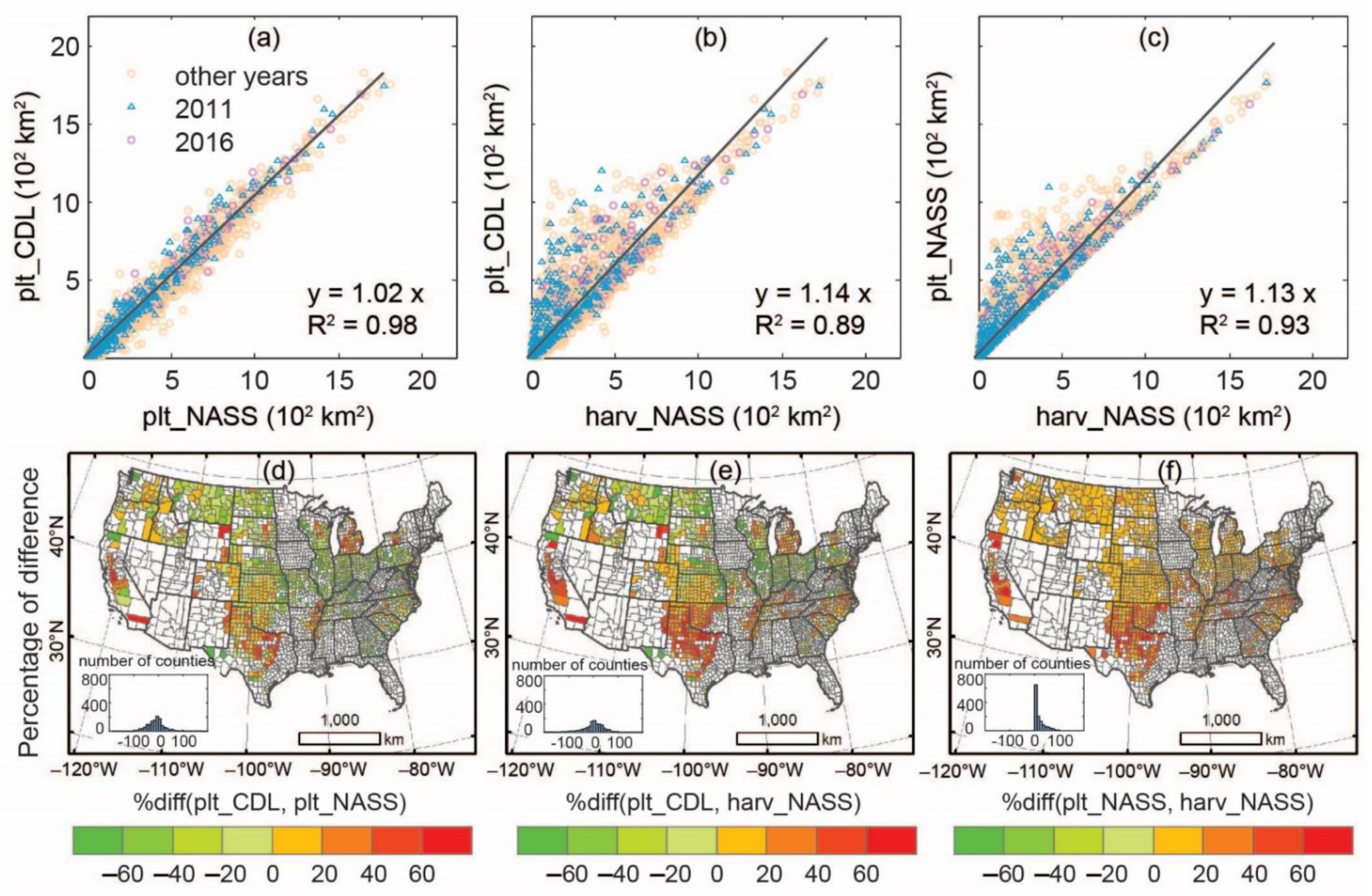
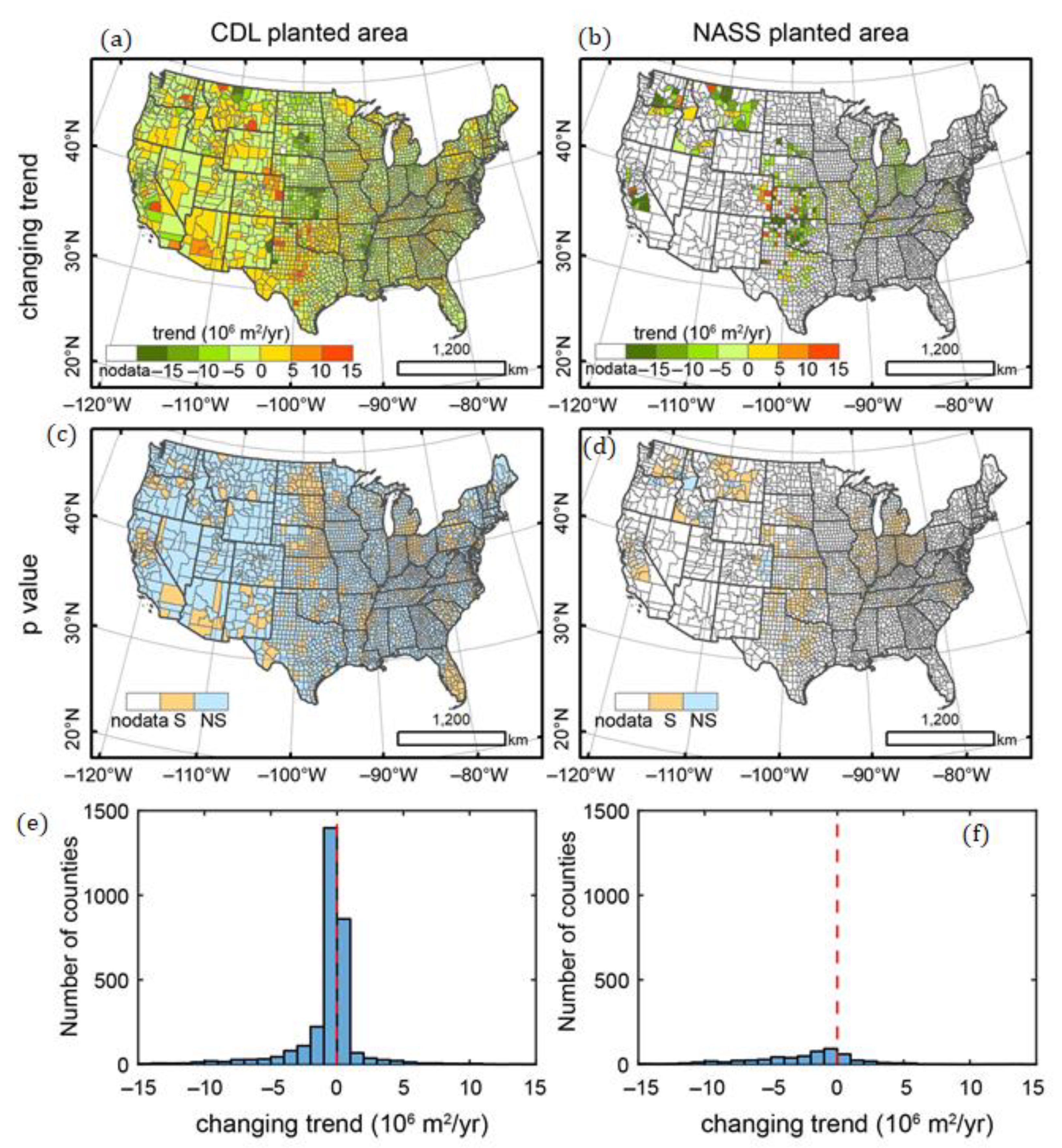
3.1. Spatiotemporal Consistency of Winter Wheat Planted and Harvested Areas from 2008–2018

At the national scale, the NASS winter wheat planted and harvested areas had three phases of changes in the study period: (1) a decrease phase from 2008–2010, (2) an increase phase from 2010–2013, and (3) a decrease phase from 2013–2018 (Figure 2a). The CDL winter wheat planted area had similar three-phase dynamics similar to the NASS planted area (Figure 1a). The disagreements between the NASS planted area and CDL planted area were relatively small for most of the years (<10%). We calculated the anomaly for the mean values of 2008–2018, and the planted area from both NASS and CDL datasets showed a significant decrease from 2013 (Figure 2b). The NASS harvested area had a similar change pattern to the planted area but with different magnitudes over the years (Figure 2b).

At the county scale, for all the counties with winter wheat planted acreages from both NASS and CDL datasets in the period of 2008–2018, winter wheat planted areas calculated from the CDL were highly consistent with those from the NASS’s officially reported dataset (R² = 0.98, p < 0.001) (Figure 3a). There are relatively small interannual variations in the slope values (<10%) and R² values among the individual years (

Table 1. A summary of the relationships among winter wheat cropping areas between the CDL and NASS datasets from 2008–2018 (plt_CDL, CDL planted area; plt_NASS, NASS planted area; harv_NASS, NASS harvested area).

Year	plt_CDL vs. plt_NASS				plt_CDL vs. harv_NASS				plt_NASS vs. harv_NASS
	Slope	R2	Bias (102 km2)	RMSE (102 km2)	Slope	R2	Bias (102 km2)	RMSE (102 km2)	Slope	R2	Bias (102 km2)	RMSE (102 km2)
2008	0.96	0.97	–12.22	280.66	1.07	0.94	3.82	266.03	1.11	0.96	16.03	280.66
2009	0.99	0.99	–6.46	306.28	1.11	0.87	16.84	286.65	1.13	0.90	23.30	306.28
2010	1.02	0.99	1.13	292.75	1.12	0.95	15.93	279.13	1.11	0.97	14.80	292.75
2011	1.02	0.99	0.75	287.00	1.15	0.86	23.09	268.17	1.14	0.90	22.34	287.00
2012	1.02	0.99	1.67	300.82	1.10	0.91	17.68	288.64	1.09	0.95	16.01	300.82
2013	1.01	0.99	–1.11	301.23	1.15	0.87	22.61	279.99	1.14	0.89	23.72	301.23
2014	0.97	0.98	–4.41	302.44	1.13	0.84	21.75	275.66	1.18	0.88	26.16	302.44
2015	1.06	0.99	5.12	321.55	1.19	0.93	26.63	303.82	1.14	0.96	21.51	321.55
2016	1.06	0.98	5.54	311.76	1.17	0.92	23.35	296.98	1.11	0.96	17.81	311.76
2017	1.07	0.97	6.33	298.89	1.21	0.87	29.65	281.70	1.15	0.94	23.31	298.89
2018	1.09	0.98	8.90	303.80	1.22	0.84	34.24	285.68	1.14	0.90	25.34	303.80

). In many counties, winter wheat harvested areas were much smaller than winter wheat planted areas (Figure 3b,c). Most of those counties with a large discrepancy between winter wheat planted area and harvested area were distributed in the Southern Great Plains and California, where some winter wheat fields were used as cool-season forage for beef cattle production (grazing or haying).

At the county scale, the interannual trends of winter wheat planted areas from 2008–2018 were calculated (Figure 4). As the NASS dataset has missing data in each year for various counties, only 626 counties were included (Figure 4b,d). According to the CDL dataset, 2168 counties had a loss of winter wheat planted area and 998 counties had a gain of winter wheat planted area (Figure 4a). There was a geographic shift of winter wheat plant area, as shown by the loss and gain of winter wheat planted area at the county scale (Figure 4a). Many counties in Kansas and the Northern Great Plains (in particular, South Dakota) had large losses of winter wheat planted area (Figure 4a). In comparison, many counties in Oklahoma, Texas, and several other midwest states had moderate to large gains of winter wheat planted area (Figure 4a). For most states, there is a reasonable spatial agreement of loss and gain of winter wheat planted area between the NASS and CDL datasets, however, in Oklahoma and Texas, there are noticeable differences between these two datasets (Figure 4a,b). A number of counties in Oklahoma and Texas had losses of winter wheat planted area according to the NASS dataset but gains of winter wheat area according to the CDL dataset. This discrepancy could be related to the imprecise estimates of winter wheat area from the CDL dataset because of image spatial resolution, misclassifications, and misalignment of field boundaries [36].

For all the counties with winter wheat grain production, from planted and harvested area data from 2008–2018, grain production had noticeably stronger relationships with harvested areas than with planted area (Figure 5) due to part of the planted acreages being used for grazing and hay.

Table 2. A summary of the relationships between county-level winter wheat grain production and cropping areas in the CONUS from 2008–2018 from the NASS and CDL datasets.

Year	prod_NASS vs. plt_CDL				prod_NASS vs. plt_NASS				prod_NASS vs. harv_NASS
	Slope	R2	Bias (103 ton)	RMSE (103 ton)	Slope	R2	Bias (103 ton)	RMSE (103 ton)	Slope	R2	Bias (103 ton)	RMSE (103 ton)
2008	257.56	0.80	5.02	74.06	251.73	0.81	5.65	73.27	293.28	0.89	1.17	79.10
2009	214.09	0.66	4.65	71.02	215.73	0.69	4.46	71.25	273.40	0.86	–2.45	80.06
2010	257.45	0.80	1.12	80.36	265.18	0.82	0.26	81.46	306.04	0.89	–4.26	87.52
2011	215.92	0.60	3.51	70.60	225.97	0.63	2.33	71.93	290.31	0.79	–5.22	81.19
2012	243.86	0.75	2.98	79.01	256.14	0.79	1.48	80.81	293.26	0.87	–3.03	86.51
2013	221.88	0.61	4.56	74.68	227.6	0.63	3.85	75.47	296.46	0.82	–4.64	85.83
2014	181.54	0.56	5.81	60.39	179.37	0.57	6.06	60.10	244.45	0.77	–1.54	69.66
2015	197.58	0.72	3.57	69.65	213.49	0.76	1.49	72.19	256.62	0.85	–4.14	79.55
2016	278.65	0.75	2.53	95.96	305.26	0.80	–0.75	100.07	359.77	0.89	–7.45	109.08
2017	244.46	0.67	1.87	83.97	275.46	0.75	–1.94	88.52	343.50	0.88	–10.30	99.43
2018	218.49	0.59	2.08	79.48	249.05	0.65	–1.73	83.93	319.78	0.8	–10.53	95.35

lists the statistics of the linear regression models (slope, R², and RMSE) between grain production and cropping areas in the period of 2008–2018, and the poorest relationship occurred in the spring drought year of 2014.

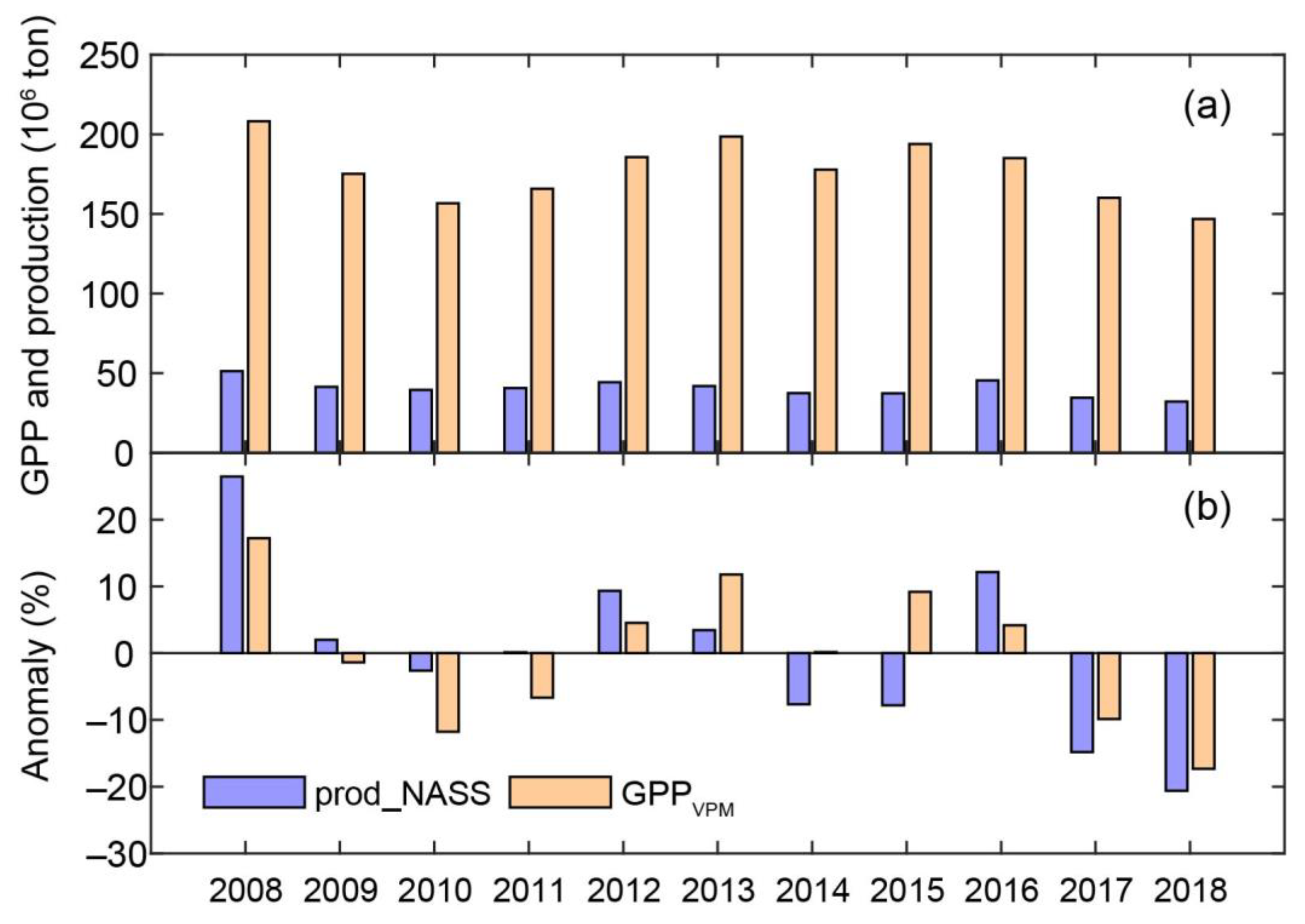
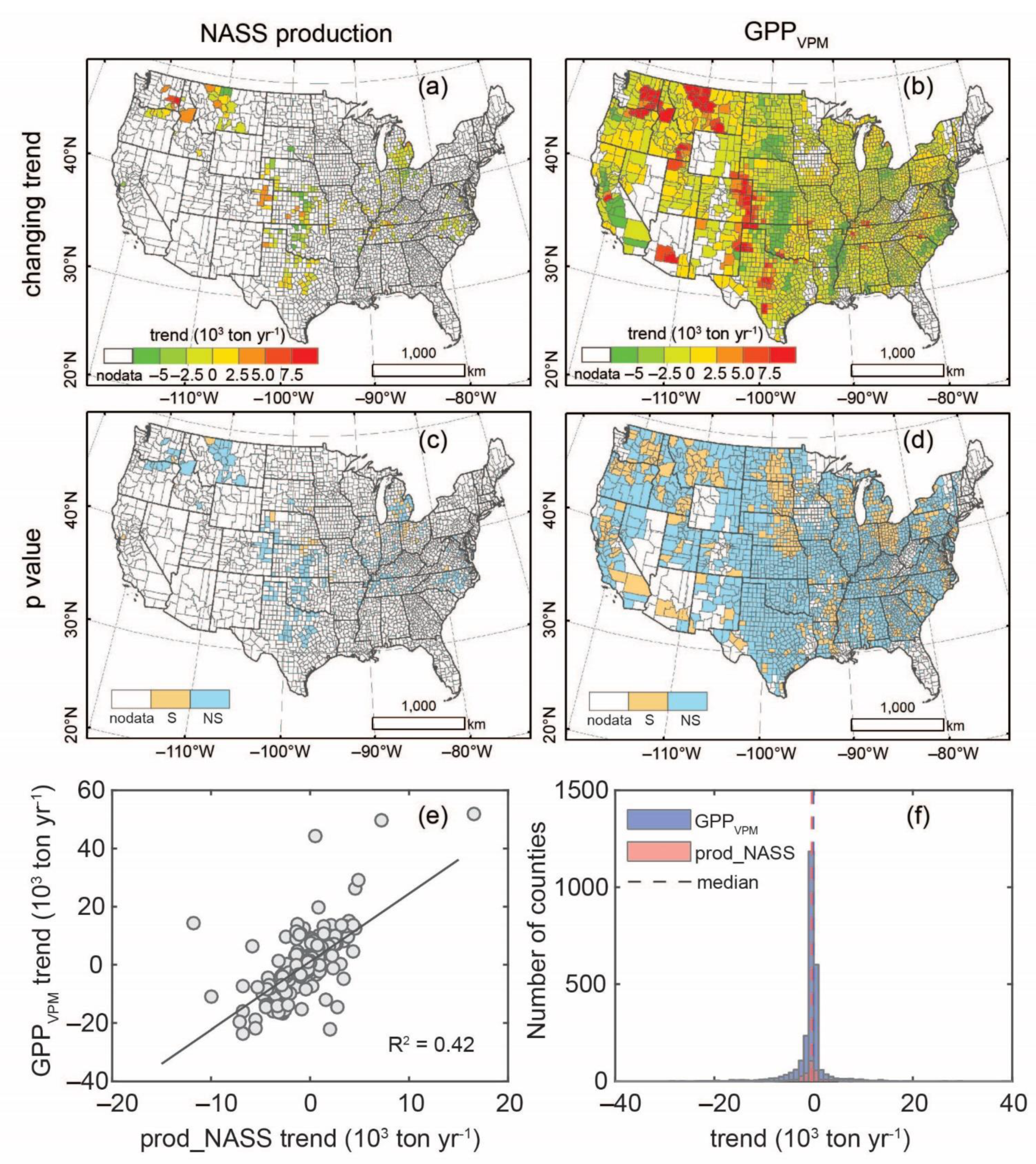
3.2. Spatiotemporal Dynamics of GPP_VPM and Grain Production from NASS Dataset from 2008–2018

At the national scale, winter wheat grain production showed a decreasing trend from 2008–2018 (Figure 6), which is largely determined by the decrease in planted and harvested area (Figure 1). GPP_VPM showed a similar decreasing trend as grain production from 2008 to 2018, but with strong response in some drought years, such as 2011 and 2014.

At the county scale, we quantified the interannual trends of GPP_VPM and grain production from 2008–2018 (Figure 7). Out of 291 counties with continuous NASS grain production data during the 11 years, winter wheat grain production showed increasing trends in 90 counties and decreasing trends in 201 counties (Figure 7a,c). The interannual trend of NASS grain production had a strong linear relationship with the that of GPP_VPM (Figure 7e). Out of 2609 counties in the CONUS, GPP_VPM data show 821 counties with a substantial increasing trend and 1788 counties with a decreasing trend (Figure 7b,d). Many counties with a decrease in GPP_VPM were located in the Great Plains (South Dakota, Kansas, Oklahoma) and the states along the Mississippi River (Figure 7b,d). Many counties in the northwestern states and the western edge of the Southern Great Plains showed an increasing trend of GPP_VPM (Figure 7b,d). The probability distributions of the interannual trends of NASS grain production and GPP_VPM were similar, with narrow ranges of normal distribution (Figure 7f).

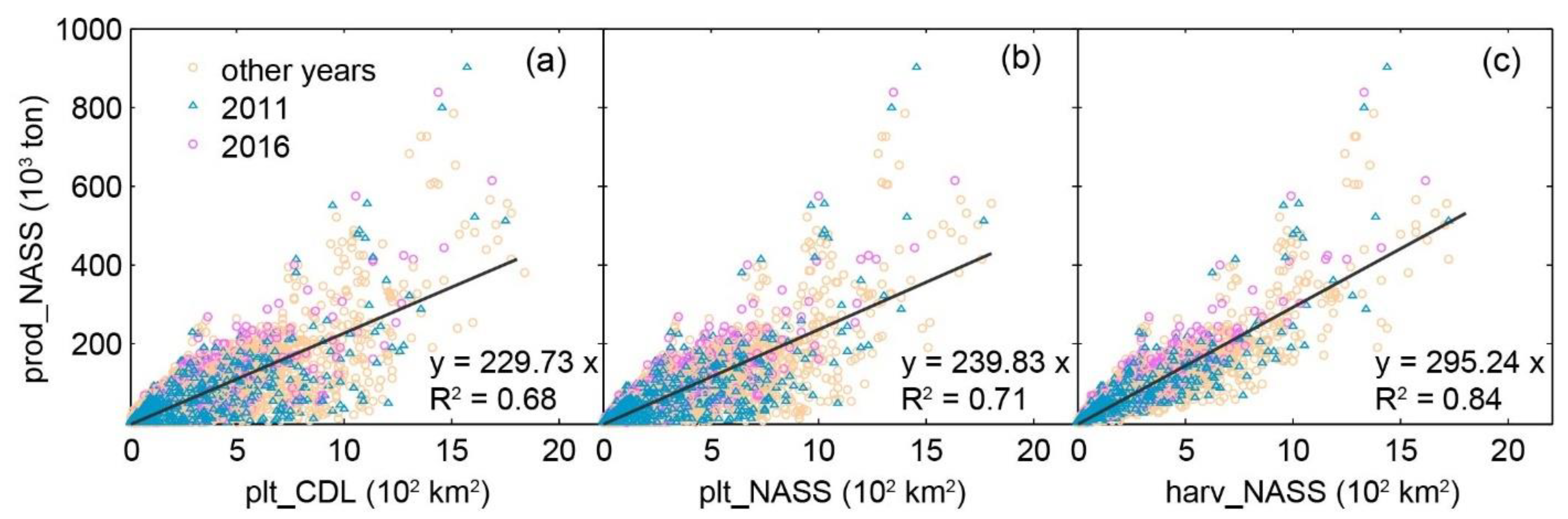
3.3. The Relationships between County-Level GPP_VPM and Winter Wheat Grain Production from 2008 to 2018

At the county scale, the relationships between GPP_VPM and winter wheat grain production from 2008 to 2018 varied from one year to another (Figure 8a), with R² values ranging from 0.59 (2008) to 0.75 (2016) (

Table 3. Statistics of linear regression results between county-level GPP_VPM and winter wheat grain production from NASS over CONUS from 2008–2018. All the counties are considered.

Year	Slope	R2	Bias (103 ton)	RMSE (103 ton)
2008	0.306	0.711	5.374	72.506
2009	0.298	0.591	4.899	69.652
2010	0.320	0.741	1.736	79.246
2011	0.343	0.688	1.404	71.655
2012	0.254	0.694	4.260	78.217
2013	0.290	0.692	3.840	76.209
2014	0.295	0.609	3.397	60.451
2015	0.229	0.660	4.071	68.616
2016	0.304	0.746	2.831	96.078
2017	0.306	0.713	0.657	84.463
2018	0.321	0.709	0.356	81.633

). The slope values in the models with no intercept (GP = HI_GPP × GPP_VPM) varied from 0.25 (2012) to 0.33 (2011) (Table 3). When all the county-year data in the CONUS were used in the linear regression model for GPP_VPM and grain production (GP), GPP_VPM could explain 68% of the variance in winter wheat grain production (Figure 8a). The relationships (Figure 8b) were also affected by the differences between the planted area calculated from CDL and harvested area from NASS statistics, which varied according to county and year (Figure 3). When including only those counties with differences less than 20% between the planted area from CDL and the harvested area from NASS, the relationship between GPP_VPM and grain production was much stronger (R² > 0.8,

Table 4. Statistics of linear regression results between county-level GPP_VPM and winter wheat grain production from NASS over CONUS from 2008–2018 by considering the relative differences between CDL-derived planted area and NASS harvested area.

Relative Difference	Slope	R2	Bias (103 ton)	RMSE (103 ton)	Number of Counties
[0,10]	0.27	0.87	0.42	113.62	3715
[10,20]	0.22	0.83	3.07	71.80	2501
[20,30]	0.17	0.79	4.48	48.47	1609
[30,40]	0.14	0.80	4.28	40.65	1076
[40,50]	0.11	0.81	3.47	34.56	691
[50,60]	0.10	0.83	3.48	38.22	519
>60	0.07	0.69	0.44	26.57	2127

).

HI_GPP values had a moderate range of variation across most of the county-years (Figure 8c), which was not affected much by the difference between the two cropping areas (Figure 8c). For those counties with small differences (<20%) between the two cropping areas, HI_GPP values ranged from 0.2–0.3 (Figure 8d). Geographically, high HI_GPP values occurred in the northern part of the CONUS, and the winter wheat belt region in the Southern Great Plains generally had a lower HI_GPP, except for part of western Kansas (Figure 9).

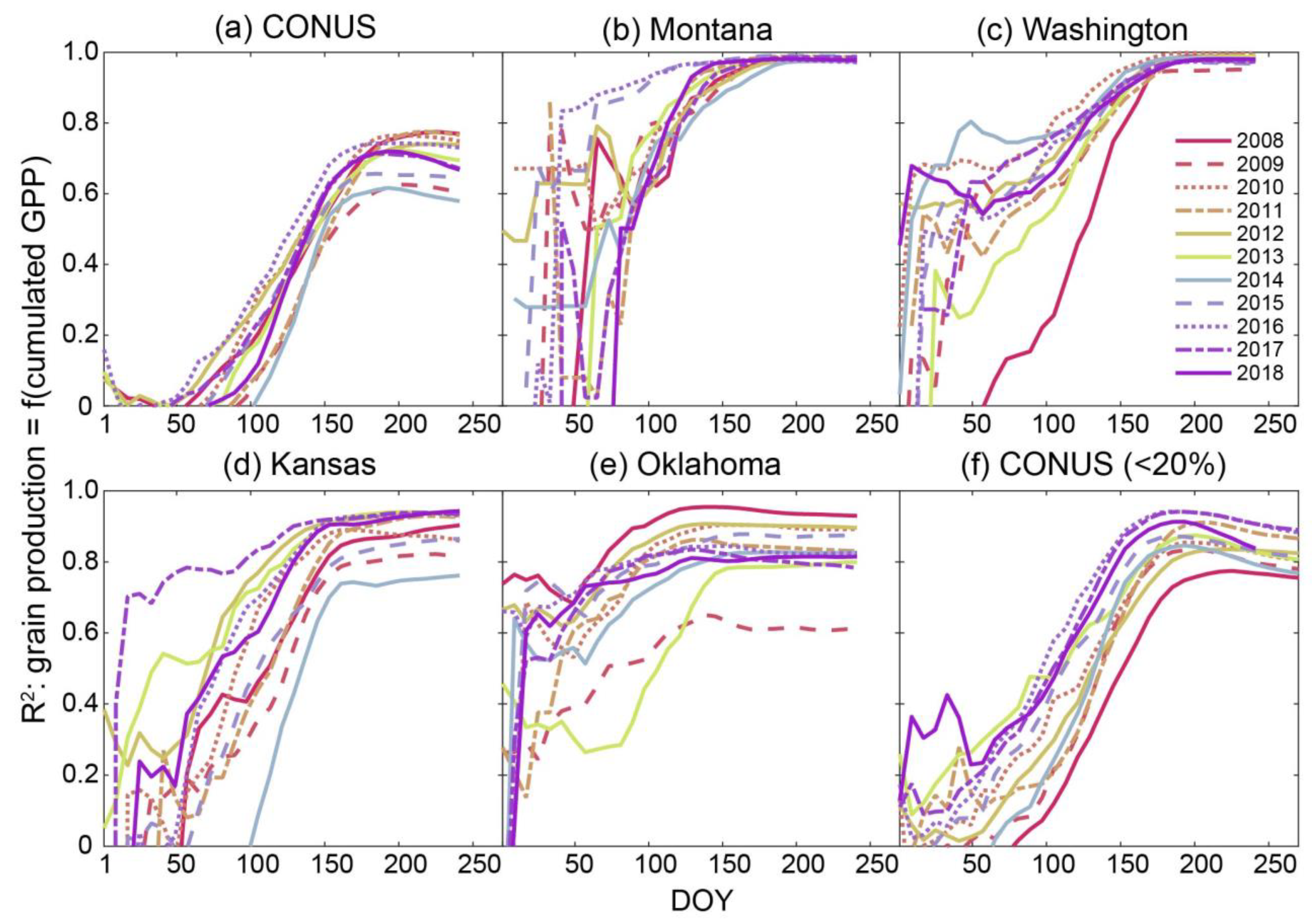
3.4. In-Season Forecasting of Winter Wheat Grain Production Using Cumulative GPP Data

In the CONUS, winter wheat is usually planted from September–November, and harvested from June–August of the following year. We assessed the potential of the simple linear regression model in forecasting grain production based on cumulative GPP. When using all the county-year data in the CONUS, the model prediction skill increased over time, reaching 60% to 80% by the end of June (Figure 10a). When using all the county-year data in a state, the model prediction skills for those states located in the cold northern part of the CONUS, where there were few differences between CDL-derived planted area and NASS harvested area, reached 90% by the end of May (Figure 10b,c). For those states located in the Southern Great Plains with big differences between the two cropping areas, that is, CDL-derived planted area and harvested area from NASS statistics, the model prediction skill varies over the years, ranging from 70% to 90% (Figure 10d,e). After excluding those counties with a difference larger than 20% between the two cropping areas, the model prediction skill for the CONUS increases and varies between 80% and 90% over the years (Figure 10f).

4. Discussion

4.1. Spatiotemporal Dynamics of Winter Wheat Planted Area, GPP, and Grain Production

Many factors contributed to the spatiotemporal changes of winter wheat planting, GPP, and grain production, including the grain market volatility (e.g., international trade market, fluctuating market price), and climate-induced variation. For international trade, the US share of global exports for wheat was ~20% before 2013, which then shrank to ~15% in recent years, driven by rising exports from Russia, the European Union, and South America [50]. The global wheat price also experienced an increase from ~5 dollars/bushel in 2008 to ~9 dollars/bushel in 2012, then decreased to ~USD 5/bushel in 2018 [51]. The interannual variation of winter wheat planted area, GPP, and grain production is highly consistent with the wheat price dynamics (Figure 2 and Figure 6). Domestically, as winter wheat is usually planted from September to October, and is harvested in June and July after maize and soybean planting, this makes it compete directly with maize and soybean. With less profit created by winter wheat over the years, maize and soybeans are preferred by US farmers. The recurring droughts throughout the Great Plains also exacerbated the shrinkage of winter wheat acreage. The 2011 drought in the Southern Great Plains and the 2017 drought in the Northern Great Plains impacted wheat growing, resulting in a large production reduction in 2012 (Figure 6). After the 2017 drought, wheat was replaced by soybean as the predominant crop in North Dakota, and more US states are increasingly planting maize and soybeans rather than wheat. For example, in Kansas, the largest wheat growing state in the US, wheat planted areas become smaller than maize and soybean areas in 2017 [52].

4.2. Spatiotemporal Consistency of Winter Wheat Cropping Areas from the CDL and NASS Datasets

Crop planted area and its spatial distribution are the first data layer for crop production monitoring and forecasting. A few studies compared the planted area derived from the CDL dataset and NASS statistics over a few years or over a few states [15,36]. The CDL pixel-based planted area estimates generally showed a satisfying accuracy for major crops (85–95% for maize, soybean, and wheat), but had a tendency of underestimation compared with NASS planted area. The pixel counting estimation of crop acreage from the CDL may underestimate crop acreages for certain counties and states but may yield overestimation for other states and counties. It should be indicated that the R² value does not indicate that the estimation is biased up or down. In this study, the winter wheat planted area estimates in the CONUS for the CDL dataset showed a strong spatiotemporal consistency (R² = 0.98) with those from the NASS dataset from 2008–2018 at the county scale (Figure 3). This high spatiotemporal consistency can be largely attributed to the accuracy of the CDL and NASS statistical data, especially for major crop types (winter wheat, soybean, and maize) [15] in the major crop production areas. The high accuracy and robustness of the CDL dataset for winter wheat planted area estimation makes it reliable for crop monitoring.

Crop harvested area and its spatial distribution were directly related to crop production because some crop fields could not be harvested due to damage, failure, and other factors. However, there is still a lack of pixel-based harvested area at a regional scale. Thus, it is important to calculate the difference between planted and harvested area for monitoring crop production. In our study, we found that the spatiotemporal consistency of winter wheat planted and harvested area in the CONUS varied substantially, especially in the Southern Great Plains and in some spring drought years (2011, 2013–2014), with a difference of more than 20% (Figure 2 and Figure 3). The Southern Great Plains are one of the key regions for the nation’s wheat and beef production. In many counties of the Southern Great Plains region, winter wheat is used as part of a dual purpose graze–grain system, serving as both a grain crop and a forage crop to supply beef cattle [35,53]. Drought is an important factor that can lead to the loss of grain yield and abandonment of winter wheat acreage in the Southern Great Plains. Winter wheat crops in this area normally break from dormancy in late February or early to mid-March. A lack of precipitation or snow before the dormancy period could significantly reduce the growth of winter wheat crops [54]. These factors could have led to the significant differences between planted and harvested area, especially over the Southern Great Plains.

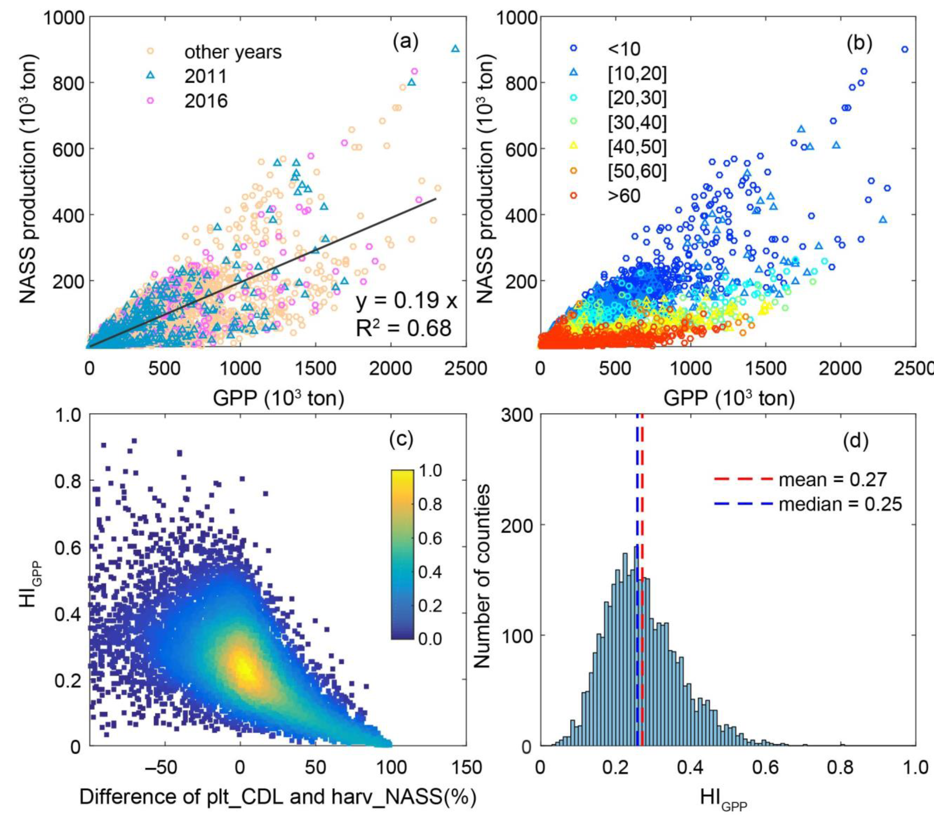
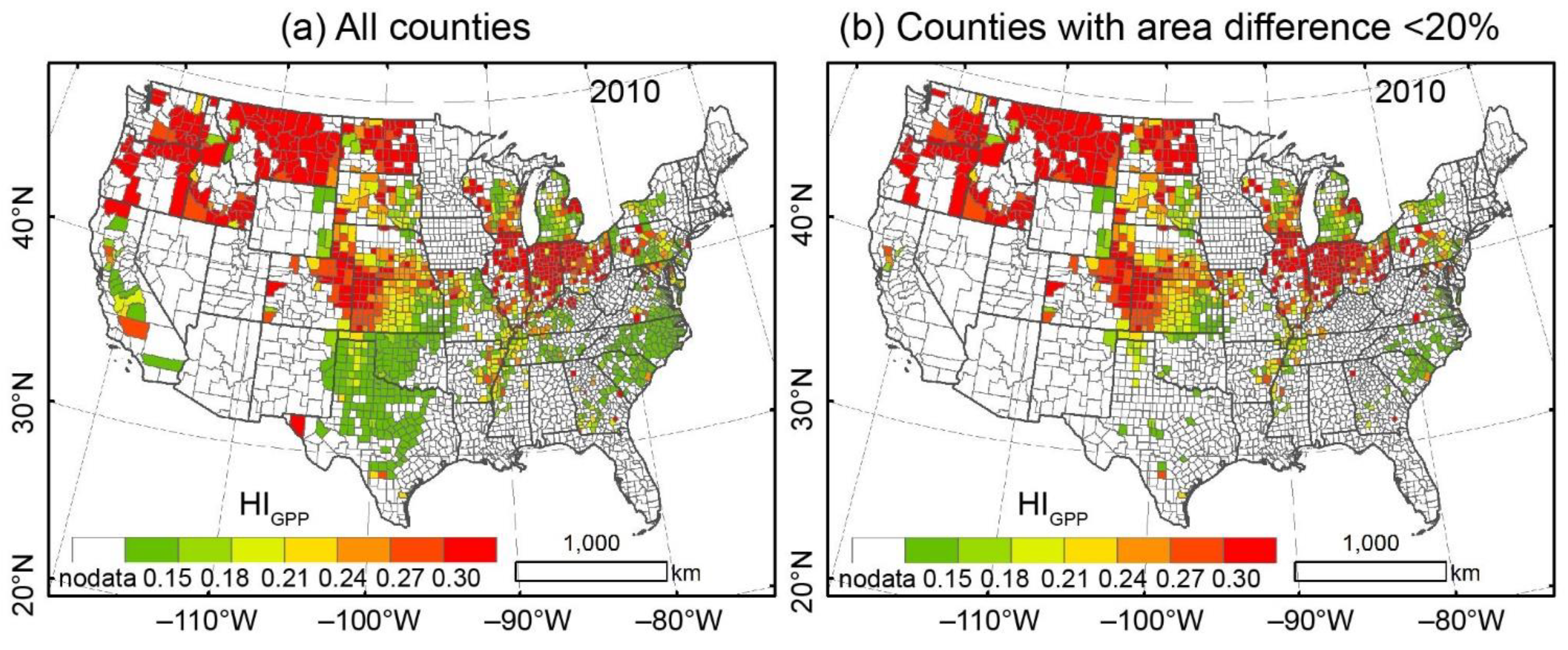
4.3. Harvest Index—The Relationship between Winter Wheat Grain Production and GPP_VPM

The “harvest index” (HI) is used in crop production research in different ways: the ratio of crop grain production over (1) aboveground biomass (AGB), namely HI_AGB [28], (2) net primary production (NPP), namely HI_NPP [27,29], and (3) gross primary production (GPP), namely HI_GPP [26,33]. These three His are different but related to each other, as GPP, NPP, and AGB are closely related. GPP represents the total carbon fixed by photosynthesis during the growing season. NPP is part of GPP, deducted by autotrophic respiration, and is often estimated as a sum of aboveground biomass and belowground biomass at harvest time. AGB is the total biomass allocated to the leaves, stems, branches, and seeds. The grain production (yield) is part of AGB at harvest.

HI_AGB derived from field-level studies showed a large variability in previous studies [28,55], which is contributed to the seed variety and growing condition. HI_NPP is usually calculated from HI_AGB and the root:shoot ratio at the field scale. The root:shoot ratio for wheat ranges from 0.19–0.21 [28,56]. For HI_GPP, Done et al. [57] and He et al. [26] reported a value of 0.29–0.37 based on modeled GPP and yield data at a regional scale. Our results showed a median HI_GPP of 0.30 from 2008–2018, and it fluctuated over counties and years (Figure 5). This variation of the GPP–yield relationship (HI_GPP) could result from environmental factors, crop management, and crop varieties (genomics). For example, winter wheat grain production in the Southern Great Plains is relatively low and more variable than for other regions, because some winter wheat fields are used as pasture for cattle grazing. The rate of abandonment could vary in some extreme climate years, as adverse weather reduces wheat yield. In addition, fertilizer application, tillage, and row spacing could also affect the yield both spatially and temporally [58]. Additional studies are needed to quantify the responses of GPP and grain production under extreme climate events.

4.4. In-Season Forecasting for Winter Wheat Grain Production

The LUE-based GPP models provide a simple but efficient way to estimate biomass or yield [59]. Unlike empirical models, they are semi-empirical and can be applied at both site or regional scales with calibration and validation [59,60]. Our study combined the GPP estimated from the VPM and CDL crop area and to predict winter wheat grain production. At the county and state scales, the predicted grain production estimates correlated well with the NASS grain production. This in-season forecasting pilot study was run at county and state scales because the NASS grain production data are readily available at those scales. Lack of access to the field-scale grain production data limits the validation of GPP_VPM-based grain production data at the field scale. GPP data at a moderate spatial resolution (500 m) were used in this study. For the major production regions of winter wheat, which produced more than 40% of the total winter wheat grain, the field sizes are usually large and there are few mixed pixels in these counties and states. However, for other regions, the mixed pixels problem can cause significant discrepancies in calculating wheat GPP and grain production. GPP products with high spatial resolutions (e.g., 30 m Landsat, and 10 m Sentinel-2) and suitable temporal frequency (weekly) may overcome the above limitations for field-scale agricultural applications.

This study highlighted the importance of accurate and in-season or annual maps of crop types for the prediction of crop production, including both planted and harvested areas. Annual or in-season maps of crop planted areas provided the basic information at the beginning of the growing season. Annual to-be-harvested area maps in the growing season would be helpful in predicting grain production as grain production is calculated as a function of “to-be-harvested” crop areas. For some major crops like maize and soybean, there could be no significant differences between planted area and harvested area in the CONUS [33]. Thus, early mapping of the planted area in the growing season could be used for grain production estimation. However, for winter wheat, our study showed that there were significant differences between planted and harvested areas over the CONUS, especially the Southern Great Plains, where the relative difference could be greater than 20%. Though numerous studies have tried to provide in-season crop type maps as early as possible based on remote sensing data [61,62], there is not much attention paid to the research of planted and harvested area mapping. A separate classification of planted area and harvested area can help to get a more accurate prediction of grain production. Another issue is to have updated (in-season) and high spatial resolution (e.g., 30 m or 10 m) crop classification maps. The CDL dataset usually has a six-month lag time after harvest, before being released to the public, and a delay of six months after harvest would preclude in-season grain production prediction. Time series satellite observations at high spatial resolutions, for example, from Sentinel-2 (5-day to 10-day revisit) and Sentinel-1 (6-day or 12-day revisit), offer rich data to map different types of crops at a field scale in a timely fashion, especially in those regions with complicated crop landscapes and frequent cloud cover.

5. Conclusions

We evaluated the spatiotemporal consistency among NASS winter wheat statistics (planted area, harvested area, grain production), CDL-derived planted area, and GPP_VPM for 2008–2018 at national and county scales. High spatiotemporal consistencies of planted area from the CDL and NASS datasets were found. There were large disagreements between the CDL planted area and NASS harvested area in many counties, especially in the SGP. The correlation between annual total GPP_VPM and grain production varied with individual counties, depending upon the differences between CDL planted area and NASS harvested area. It was found that the cumulative GPP_VPM at an 8-day interval and HI_GPP were able to accurately predict winter wheat grain production at the county scale from early May to late June. HI_GPP, calculated as the ratio of grain production over GPP, varied over a small range over different counties and years, when excluding those counties with large differences of CDL planted and NASS harvested areas, with a median value of 0.27. The results from this study highlight the importance of differentiating planted area and harvested area in crop mapping. Our results also demonstrate the potential of using GPP_VPM products in estimating and monitoring grain production of winter wheat in the CONUS.

References

1. Mitchell, D.O.; Mielke, M. Wheat: The global market, policies, and priorities. Glob. Agric. Trade Dev. Ctries. 2005, 195–214. [Google Scholar]
2. USDA FAS. World Agricultural Production; USDA, Ed.; USDA Foreign Agriculture Service: Washington, DC, USA, 2020.
3. USDA NASS. USDA Crop Production 2014 Summary; USDA: Washington, DC, USA, 2014; Volume 1.
4. ADB. Results of the Methodological Studies for Agricultural and Rural Statistics; Asian Development Bank: Mandaluyong City, Philippines, 2015. [Google Scholar]
5. Carfagna, E.; Carfagna, A. Alternative Sampling Frames and Administrative Data. What is the Best Data Source for Agricultural Statistics? Agric. Surv. Methods 2010. [Google Scholar] [CrossRef]
6. USDA NASS. The Yield Forecasting Program of NASS; USDA, Ed.; NASS Staff Report No. SMB 12-01; USDA: Washington, DC, USA, 2012.
7. USDA NASS/WAOB. Understanding USDA Crop Forecasts; USDA, Ed.; Miscellaneous Publication: Washington, DC, USA, 1999; No.1554.
8. De Groote, H.; Traore, O. The cost of accuracy in crop area estimation. Agric. Syst. 2005, 84, 21–38. [Google Scholar] [CrossRef] [Green Version]
9. Mulla, D.J. Twenty five years of remote sensing in precision agriculture: Key advances and remaining knowledge gaps. Biosyst. Eng. 2013, 114, 358–371. [Google Scholar] [CrossRef]
10. Shelestov, A.; Lavreniuk, M.; Kussul, N.; Novikov, A.; Skakun, S. Exploring Google Earth Engine Platform for Big Data Processing: Classification of Multi-Temporal Satellite Imagery for Crop Mapping. Front. Earth Sci. 2017, 5, 1–10. [Google Scholar] [CrossRef] [Green Version]
11. Orynbaikyzy, A.; Gessner, U.; Conrad, C. Crop type classification using a combination of optical and radar remote sensing data: A review. Int. J. Remote Sens. 2019, 40, 6553–6595. [Google Scholar] [CrossRef]
12. Massey, R.; Sankey, T.T.; Congalton, R.G.; Yadav, K.; Thenkabail, P.S.; Ozdogan, M.; Sánchez Meador, A.J. MODIS phenology-derived, multi-year distribution of conterminous U.S. crop types. Remote Sens. Environ. 2017, 198, 490–503. [Google Scholar] [CrossRef]
13. Zhong, L.; Hu, L.; Zhou, H.; Tao, X. Deep learning based winter wheat mapping using statistical data as ground references in Kansas and northern Texas, US. Remote Sens. Environ. 2019, 233, 111411. [Google Scholar] [CrossRef]
14. Skakun, S.; Franch, B.; Vermote, E.; Roger, J.-C.; Becker-Reshef, I.; Justice, C.; Kussul, N. Early season large-area winter crop mapping using MODIS NDVI data, growing degree days information and a Gaussian mixture model. Remote Sens. Environ. 2017, 195, 244–258. [Google Scholar] [CrossRef]
15. Boryan, C.; Yang, Z.; Mueller, R.; Craig, M. Monitoring US agriculture: The US Department of Agriculture, National Agricultural Statistics Service, Cropland Data Layer Program. Geocarto Int. 2011, 26, 341–358. [Google Scholar] [CrossRef]
16. Lobell, D.B.; Azzari, G.; Burke, M.; Gourlay, S.; Jin, Z.; Kilic, T.; Murray, S. Eyes in the Sky, Boots on the Ground: Assessing Satellite- and Ground-Based Approaches to Crop Yield Measurement and Analysis. Am. J. Agric. Econ. 2020, 102, 202–219. [Google Scholar] [CrossRef]
17. Guan, K.Y.; Wu, J.; Kimball, J.S.; Anderson, M.C.; Frolking, S.; Li, B.; Hain, C.R.; Lobe, D.B. The shared and unique values of optical, fluorescence, thermal and microwave satellite data for estimating large-scale crop yields. Remote Sens. Environ. 2017, 199, 333–349. [Google Scholar] [CrossRef] [Green Version]
18. Deines, J.M.; Patel, R.; Liang, S.; Dado, W.; Lobell, D.B. A million kernels of truth: Insights into scalable satellite maize yield mapping and yield gap analysis from an extensive ground dataset in the US Corn Belt. Remote Sens. Environ. 2021, 253, 112174. [Google Scholar] [CrossRef]
19. Karthikeyan, L.; Chawla, I.; Mishra, A.K. A review of remote sensing applications in agriculture for food security: Crop growth and yield, irrigation, and crop losses. J. Hydrol. 2020, 586. [Google Scholar] [CrossRef]
20. Zhuo, W.; Huang, J.X.; Li, L.; Zhang, X.D.; Ma, H.Y.; Gao, X.R.; Huang, H.; Xu, B.D.; Xiao, X.M. Assimilating Soil Moisture Retrieved from Sentinel-1 and Sentinel-2 Data into WOFOST Model to Improve Winter Wheat Yield Estimation. Remote Sens. 2019, 11, 1618. [Google Scholar] [CrossRef] [Green Version]
21. Cai, Y.; Guan, K.; Lobell, D.; Potgieter, A.B.; Wang, S.; Peng, J.; Xu, T.; Asseng, S.; Zhang, Y.; You, L.; et al. Integrating satellite and climate data to predict wheat yield in Australia using machine learning approaches. Agric. For. Meteorol. 2019, 274, 144–159. [Google Scholar] [CrossRef]
22. Becker-Reshef, I.; Vermote, E.; Lindeman, M.; Justice, C. A generalized regression-based model for forecasting winter wheat yields in Kansas and Ukraine using MODIS data. Remote Sens. Environ. 2010, 114, 1312–1323. [Google Scholar] [CrossRef]
23. Wang, Y.L.; Xu, X.G.; Huang, L.S.; Yang, G.J.; Fan, L.L.; Wei, P.F.; Chen, G. An Improved CASA Model for Estimating Winter Wheat Yield from Remote Sensing Images. Remote Sens. 2019, 11, 1088. [Google Scholar] [CrossRef] [Green Version]
24. Kern, A.; Barcza, Z.; Marjanovic, H.; Arendas, T.; Fodor, N.; Bonis, P.; Bognar, P.; Lichtenberger, J. Statistical modelling of crop yield in Central Europe using climate data and remote sensing vegetation indices. Agric. For. Meteorol. 2018, 260, 300–320. [Google Scholar] [CrossRef]
25. Franch, B.; Vermote, E.F.; Becker-Reshef, I.; Claverie, M.; Huang, J.; Zhang, J.; Justice, C.; Sobrino, J.A. Improving the timeliness of winter wheat production forecast in the United States of America, Ukraine and China using MODIS data and NCAR Growing Degree Day information. Remote Sens. Environ. 2015, 161, 131–148. [Google Scholar] [CrossRef]
26. He, M.; Kimball, J.; Maneta, M.P.; Maxwell, B.; Moreno, A.; Begueria, S.; Wu, X. Regional crop gross primary productivity and yield estimation using fused Landsat-MODIS data. Remote Sens. 2018, 10, 372. [Google Scholar] [CrossRef] [Green Version]
27. Guan, K.; Berry, J.A.; Zhang, Y.; Joiner, J.; Guanter, L.; Badgley, G.; Lobell, D.B. Improving the monitoring of crop productivity using spaceborne solar-induced fluorescence. Glob. Chang. Biol. 2016, 22, 716–726. [Google Scholar] [CrossRef]
28. Prince, S.D.; Haskett, J.; Steininger, M.; Strand, H.; Wright, B. Net primary production of U.S. midwest croplands from agricultural harvest yield data. Ecol. Indic. 2001, 11, 1194–1205. [Google Scholar] [CrossRef]
29. Lobell, D.B.; Hicke, J.A.; Asner, G.P.; Field, C.; Tucker, C.; Los, S. Satellite estimates of productivity and light use efficiency in United States agriculture, 1982–1998. Glob. Chang. Biol. 2002, 8, 722–735. [Google Scholar] [CrossRef]
30. Wu, X.C.; Xiao, X.M.; Zhang, Y.; He, W.; Wolf, S.; Chen, J.Q.; He, M.Z.; Gough, C.M.; Qin, Y.W.; Zhou, Y.L.; et al. Spatiotemporal Consistency of Four Gross Primary Production Products and Solar-Induced Chlorophyll Fluorescence in Response to Climate Extremes Across CONUS in 2012. J. Geophys. Res. Biogeosci. 2018, 123, 3140–3161. [Google Scholar] [CrossRef]
31. Zhang, Y.; Xiao, X.; Wu, X.; Zhou, S.; Zhang, G.; Qin, Y.; Dong, J. A global moderate resolution dataset of gross primary production of vegetation for 2000–2016. Sci. Data 2017, 4, 1–13. [Google Scholar] [CrossRef] [PubMed] [Green Version]
32. Running, S.; Nemani, R.; Heinsch, F.A.; Zhao, M.; Reeves, M.; Hashimoto, H. A contiguous satellite-derived measure of global terrestrial primary production. Bioscience 2004, 54, 547–560. [Google Scholar] [CrossRef]
33. Wu, X.C.; Xiao, X.; Yang, Z.; Wang, J.; Steiner, J.; Bajgain, R. Spatial-temporal dynamics of maize and soybean planted area, harvested area, gross primary production, and grain production in the Contiguous United States during 2008–2018. Agric. For. Meteorol. 2020, 297, 108240. [Google Scholar] [CrossRef]
34. Steiner, J.L.; Schneider, J.M.; Pope, C.; Steele, R.F. Southern Plains Assessment of Vulnerability and Preliminary Adaptation and Mitigation Strategies for Farmers, Ranchers and Forest Land Owners; Anderson, T., Ed.; United States Department of Agriculture: Washington DC, USA, 2015; p. 61.
35. Edwards, J.T.; Carver, B.F.; Horn, G.W.; Payton, M.E. Impact of Dual-Purpose Management on Wheat Grain Yield. Crop. Sci. 2011, 51, 2181–2185. [Google Scholar] [CrossRef]
36. Lark, T.J.; Mueller, R.; Johnson, D.M.; Gibbs, H.K. Measuring land-use and land-cover change using the U.S. department of agriculture’s cropland data layer: Cautions and recommendations. Int. J. Appl. Earth Obs. Geoinf. 2017, 62, 224–235. [Google Scholar] [CrossRef]
37. Lark, T.J.; Spawn, S.A.; Bougie, M.; Gibbs, H.K. Cropland expansion in the United States produces marginal yields at high costs to wildlife. Nat. Commun. 2020, 11, 1–11. [Google Scholar] [CrossRef] [PubMed]
38. Wright, C.K.; Wimberly, M.C. Recent land use change in the Western Corn Belt threatens grasslands and wetlands. Proc. Natl. Acad. Sci. USA 2013, 110, 4134–4139. [Google Scholar] [CrossRef] [PubMed] [Green Version]
39. Wang, C.; Zhong, C.; Yang, Z.W. Assessing bioenergy-driven agricultural land use change and biomass quantities in the U.S. Midwest with MODIS time series. J. Appl. Remote Sens. 2014, 8, 085198. [Google Scholar] [CrossRef] [Green Version]
40. Han, W.G.; Yang, Z.; Di, L.P.; Mueller, R. CropScape: A Web service based application for exploring and disseminating US conterminous geospatial cropland data products for decision support. Comput. Electron. Agric. 2012, 84, 111–123. [Google Scholar] [CrossRef]
41. Xiao, X.M.; Hollinger, D.; Aber, J.; Goltz, M.; Davidson, E.A.; Zhang, Q.Y.; Moore, B. Satellite-based modeling of gross primary production in an evergreen needleleaf forest. Remote Sens. Environ. 2004, 89, 519–534. [Google Scholar] [CrossRef]
42. Xiao, X.M.; Zhang, Q.Y.; Braswell, B.; Urbanski, S.; Boles, S.; Wofsy, S.; Berrien, M.; Ojima, D. Modeling gross primary production of temperate deciduous broadleaf forest using satellite images and climate data. Remote Sens. Environ. 2004, 91, 256–270. [Google Scholar] [CrossRef]
43. Yan, H.; Fu, Y.L.; Xiao, X.; He, Q.H.; He, H.L.; Ediger, L. Modeling gross primary productivity for winter wheat–maize double cropping system using MODIS time series and CO2 eddy flux tower data. Agric. Ecosyst. Environ. 2009, 129, 391–400. [Google Scholar] [CrossRef]
44. Doughty, R.; Xiao, X.; Wu, X.; Zhang, Y.; Bajgain, R.; Zhou, Y.; Qin, Y.; Zou, Z.; McCarthy, H.; Friedman, J.; et al. Responses of gross primary production of grasslands and croplands under drought, pluvial, and irrigation conditions during 2010–2016, Oklahoma, USA. Agric. Water Manag. 2018, 204, 47–59. [Google Scholar] [CrossRef]
45. Dong, J.W.; Xiao, X.M.; Wagle, P.; Zhang, G.L.; Zhou, Y.T.; Jin, C.; Torn, M.S.; Meyers, T.P.; Suyker, A.E.; Wang, J.B.; et al. Comparison of four EVI-based models for estimating gross primary production of maize and soybean croplands and tallgrass prairie under severe drought. Remote Sens. Environ. 2015, 162, 154–168. [Google Scholar] [CrossRef] [Green Version]
46. Jin, C.; Xiao, X.M.; Wagle, P.; Griffis, T.; Dong, J.W.; Wu, C.Y.; Qin, Y.W.; Cook, D.R. Effects of in-situ and reanalysis climate data on estimation of cropland gross primary production using the Vegetation Photosynthesis Model. Agric. For. Meteorol. 2015, 213, 240–250. [Google Scholar] [CrossRef] [Green Version]
47. Xin, F.F.; Xiao, X.M.; Zhao, B.; Miyata, A.; Baldocchi, D.; Knox, S.; Kang, M.; Shim, K.M.; Min, S.; Chen, B.Q.; et al. Modeling gross primary production of paddy rice cropland through analyses of data from CO2 eddy flux tower sites and MODIS images. Remote Sens. Environ. 2017, 190, 42–55. [Google Scholar] [CrossRef] [Green Version]
48. Kalfas, J.L.; Xiao, X.; Vanegas, D.X.; Verma, S.B.; Suyker, A.E. Modeling gross primary production of irrigated and rain-fed maize using MODIS imagery and CO2 flux tower data. Agric. For. Meteorol. 2011, 151, 1514–1528. [Google Scholar] [CrossRef] [Green Version]
49. Xin, F.F.; Xiao, X.M.; Cabral, O.M.R.; White, P.M.; Guo, H.Q.; Ma, J.; Li, B.; Zhao, B. Understanding the Land Surface Phenology and Gross Primary Production of Sugarcane Plantations by Eddy Flux Measurements, MODIS Images, and Data-Driven Models. Remote Sens. 2020, 12, 2186. [Google Scholar] [CrossRef]
50. Bond, J.K. Wheat Outlook: May 2020. In Wheat Sector at a Glance; USDA ERS: Washington, DC, USA, 2020. [Google Scholar]
51. Widmar, D. Disappointing Wheat Prices Headed into 2020. Agric. Econ. Insights 2019. Available online: https://aei.ag/2019/10/07/disappoint-wheat-prices-headed-into-2020/ (accessed on 28 April 2021).
52. USDA NASS. USDA Crop Production 2017 Summary; USDA, Ed.; USDA, National Agricultural Statistics Service: Washington, DC, USA, 2017; Volume 1.
53. Hossain, I.; Epplin, F.M.; Horn, G.W.; Krenzer, E.G. Wheat Production and Management Practices Used by Oklahoma Grain and Livestock Producers; Bulletin 818 Oklahoma State University Cooporation Extension Service: Stillwater, OK, USA, 2004. [Google Scholar]
54. Steiner, J.L.; Briske, D.D.; Brown, D.P.; Rottler, C.M. Vulnerability of Southern Plains agriculture to climate change. Clim. Chang. 2018, 146, 201–218. [Google Scholar] [CrossRef] [Green Version]
55. Hay, R.K.M. Harvest Index—A Review of Its Use in Plant-Breeding and Crop Physiology. Ann. Appl. Biol. 1995, 126, 197–216. [Google Scholar] [CrossRef]
56. Monfreda, C.; Ramankutty, N.; Foley, J.A. Farming the planet: 2. Geographic distribution of crop areas, yields, physiological types, and net primary production in the year 2000. Glob. Biogeochem. Cycles 2008, 22. [Google Scholar] [CrossRef]
57. Dong, J.; Lu, H.B.; Wang, Y.W.; Ye, T.; Yuan, W.P. Estimating winter wheat yield based on a light use efficiency model and wheat variety data. ISPRS J. Photogramm. Remote Sens. 2020, 160, 18–32. [Google Scholar] [CrossRef]
58. Vocke, G.; Ali, M.U.S. Wheat Production Practices, Costs, and Yields: Variations Across Regions; Department of Agriculture Economic Research Service: Washington DC, USA, 2013; p. E1b-116.
59. Yuan, W.; Chen, Y.; Xia, J.; Dong, W.; Magliulo, V.; Moors, E.; Olesen, J.E.; Zhang, H. Estimating crop yield using a satellite-based light use efficiency model. Ecol. Indic. 2016, 60, 702–709. [Google Scholar] [CrossRef] [Green Version]
60. Marshall, M.; Tu, K.; Brown, J. Optimizing a remote sensing production efficiency model for macro-scale GPP and yield estimation in agroecosystems. Remote Sens. Environ. 2018, 217, 258–271. [Google Scholar] [CrossRef]
61. Cai, Y.; Guan, K.; Peng, J.; Wang, S.; Seifert, C.; Wardlow, B.; Li, Z. A high-performance and in-season classification system of field-level crop types using time-series Landsat data and a machine learning approach. Remote Sens. Environ. 2018, 210, 35–47. [Google Scholar] [CrossRef]
62. Qiu, B.; Luo, Y.; Tang, Z.; Chen, C.; Lu, D.; Huang, H.; Chen, Y.; Chen, N.; Xu, W. Winter wheat mapping combining variations before and after estimated heading dates. ISPRS J. Photogramm. Remote Sens. 2017, 123, 35–46. [Google Scholar] [CrossRef]
Figure 1. Annual maps of county-level winter wheat over CONUS for year 2010: (a) CDL-derived planted area (plt_CDL), (b) NASS planted area (plt_NASS), (c) NASS harvested area (harv_NASS), (d) NASS grain yield, (e) NASS grain production, and (f) annual averaged GPPVPM of winter wheat.
Remotesensing 13 01735 g001
Figure 2. Interannual changes of winter wheat planted and harvested areas in the CONUS from 2008–2018 (plt_CDL, plt_NASS, harv_NASS): (a) planted area and harvested area; (b) anomalies of planted area and harvested area for the multi-year averages from 2008–2018.
Remotesensing 13 01735 g002
Figure 3. Comparisons between winter wheat planted areas and harvested area over CONUS from 2008–2018 at the county scale from the CDL and NASS datasets (plt_CDL, plt_NASS, harv_NASS). (a) Planted area, (b,c) planted area vs. harvested area, (df) the spatial discrepancy (relative difference, %) in 2010 for planted area (d), and between planted area and harvested area (e,f). Year 2011 is a typical drought year over the winter wheat belt, and 2016 is a wet year.
Remotesensing 13 01735 g003
Figure 4. The distributions of interannual trends of county-level winter wheat planted area over CONUS between 2008 and 2018 derived from the CDL and NASS datasets. (a) Trends from the CDL dataset, (b) trends from the NASS dataset, (c) p-value for the CDL dataset, S: significant, p-value < 0.05, NS: not significant, p-value > 0.05, (d) p-value for the NASS data, (e) the relationships between the trends of planted areas calculated from CDL and NASS, (f) the histograms of the trends of planted areas calculated from CDL and NASS.
Remotesensing 13 01735 g004
Figure 5. The relationships between county-level winter wheat grain production and cropping areas in the CONUS from 2008 to 2018 from the CDL and NASS datasets (plt_CDL, plt_NASS, harv_NASS). (a) Grain production versus CDL planted area, (b) grain production versus NASS planted area, and (c) grain production versus NASS harvested area. The black solid line is the linear regression result for all the counties from 2008 to 2018.
Remotesensing 13 01735 g005
Figure 6. Interannual changes of (a) NASS winter wheat grain production (prod_NASS) and total GPP estimated from VPM (GPPVPM), (b) anomalies of prod_NASS and GPPVPM for the mean of 2008–2018.
Remotesensing 13 01735 g006
Figure 7. Interannual trends of NASS winter wheat grain production (prod_NASS) and GPPVPM from 2008–2018 in the CONUS at a county scale. (a) Changing trend for NASS grain production from 2008–2018; (b) changing trend for GPPVPM from 2008–2018; (c) p-value of the linear regression model for calculation of NASS grain production trends, S means significant trend with p < 0.05, and NS means not significant trend with p > 0.05; (d) similar to (c), but for the trend of GPPVPM; (e) linear regression between the trend of NASS grain production and of GPPVPM for those counties with continuous NASS grain production and GPPVPM data from 2008–2018; (f) histograms for the trend of NASS grain production and of GPPVPM.
Remotesensing 13 01735 g007
Figure 8. (a) The relationships between county-level winter wheat GPPVPM and grain production in the CONUS from 2008 to 2018, labeled by year, and the black solid line is the linear regression results for all the county-year data. (b) Linear regression between GPPVPM and NASS grain production from 2008 to2018, labeled by the relative difference between CDL-derived planted area (plt_CDL) and NASS harvested area (harv_NASS). (c) Density plot of the relationship between HIGPP and the difference between plt_CDL and harv_NASS. (d) Histogram of HIGPP for all the county-years with a difference of plt_CDL and harv_NASS less than <20%.
Remotesensing 13 01735 g008
Figure 9. Spatial distribution of harvest index derived from GPPVPM and NASS grain production (HIGPP) in 2010 for (a) all the counties and (b) counties with small differences (<20%) between CDL-derived planted area and NASS harvested area.
Remotesensing 13 01735 g009
Figure 10. The prediction skill of the linear regression models that predict county-level crop grain production from NASS statistics by using accumulative GPP estimates over time (8-day interval) from the VPM and CDL cropping area over the years for winter wheat from 2008–2018 over (a) all counties in CONUS; (b) all counties in Montana; (c) all counties in Washington; (d) all counties in Kansas; (e) all counties in Oklahoma; (f) CONUS for all counties with differences less than 20% between CDL-derived planted area and NASS harvested area.
Remotesensing 13 01735 g010