Sea Ice Classification of SAR Imagery Based on Convolution Neural Networks

Abstract

We explore new and existing convolutional neural network (CNN) architectures for sea ice classification using Sentinel-1 (S1) synthetic aperture radar (SAR) data by investigating two key challenges: binary sea ice versus open-water classification, and a multi-class sea ice type classification. The analysis of sea ice in SAR images is challenging because of the thermal noise effects and ambiguities in the radar backscatter for certain conditions that include the reflection of complex information from sea ice surfaces. We use manually annotated SAR images containing various sea ice types to construct a dataset for our Deep Learning (DL) analysis. To avoid contamination between classes we use a combination of near-simultaneous SAR images from S1 and fine resolution cloud-free optical data from Sentinel-2 (S2). For the classification, we use data augmentation to adjust for the imbalance of sea ice type classes in the training data. The SAR images are divided into small patches which are processed one at a time. We demonstrate that the combination of data augmentation and training of a proposed modified Visual Geometric Group 16-layer (VGG-16) network, trained from scratch, significantly improves the classification performance, compared to the original VGG-16 model and an ad hoc CNN model. The experimental results show both qualitatively and quantitatively that our models produce accurate classification results.

1. Introduction

Sea ice is a key environmental factor [1] that significantly affects polar ecosystems. Over the past decade, the Arctic has experienced dramatic climate change that affects its environment, ecology, and meteorology. The trends are more pronounced than in other regions, and this has been called the Arctic amplification [2] resulting in increasingly variable Arctic weather and sea ice conditions. These are already more extreme than at lower latitudes, and present challenges and threats to maritime operations related to resource exploitation, fisheries, and tourism in the northern areas [3,4]. Therefore, reliable and continuous monitoring of sea ice dynamics, coverage, and the distribution of ice types is important for safe and efficient operations, in addition to supporting detection of how the conditions are changing over longer timescales [5,6]. For example, Ren et al. [7] classified sea ice and open water from synthetic aperture radar (SAR) images using the U-Net model, and integrated a dual-attention mechanism into the original U-Net to improve the feature representations. Han et al. [8] introduced a method for sea ice image classification based on feature extraction and a feature-level fusion of heterogeneous data from SAR and optical images. Song et al. [9] proposed a method based on the combination of spatial and temporal features, derived from residual convolutional neural networks (ResNet) and long short-term memory (LSTM) networks that allowed the extraction of spatial feature vectors for a time series of sea-ice samples using a trained ResNet network. Then, using the feature vectors as inputs, the LSTM network further learnt the temporal variation of the set of sea-ice samples. Subsequently, they fed the high-level features into a Softmax classifier to output the most recent ice type.

For sea ice data analysis, SAR imaging plays a key role as the images acquired by air and satellite-borne platforms provide information that is not restricted by environmental factors and, importantly for Arctic monitoring, can continue to be collected during all weather conditions and through the polar night [10].

Recently, Deep Learning (DL) based methods have shown promising results in many application areas, including computer vision [11], information theory [12], and natural language processing [13]. These have been shown to have excellent generalization capabilities, particularly when properly trained on large datasets. These developments have therefore led to a belief that deep neural networks (DNNs) could lead to a significant improvement of automatic sea ice classification, considering the specific challenges related to this task. However, no applications based on this approach have yet made it into operational use.

In our paper, we explore the performance and efficiency of some DL-based methods for sea ice classification from SAR imagery. DNNs are trainable multi-layer architectures composed of multiple feature-extraction stages, succeeded by a fully connected classification module. DNNs may consist of hundreds of layers, and their architecture can be feed-forward or recurrent, having different types of layers and activation functions, and the training can be achieved through many different optimization strategies. A DNN can be built from different combinations of fully connected, convolutional, maxpooling (sub-sampling), or recurrent layers. Due to their deep nature, they are often trained on large datasets, and in general are able to achieve low generalization errors.

A convolutional neural network (CNN) [14,15] is a feed-forward network consisting of only convolutional layers, pooling layers, and fully connected layers. A CNN [16] is the type of DNN which is most commonly applied to analyzing visual imagery. In the convolutional layers, a CNN extracts features from the image in a hierarchical way by using multiple filters. Each filter consists of a set of weight parameters, which are iteratively adjusted and optimised using an optimization algorithm. These filters are applied to an input image to create a feature map that summarizes the presence of detected features in the input. The CNN learns the filter coefficients during training in the context of the specific problem, and uses pooling layers to sub-sample the output in such a way that the most prominent pixels are propagated to the next layer, dropping the rest. Here it provides a fixed sized output matrix, which is translation and rotation invariant.

Sea ice classification based on SAR imagery is a very challenging task because, in addition to the sea ice characteristics, the radar signals are sensitive to imaging geometry, speckle noise [17], and the blurring of edges and strong anisotropies that may be produced by the SAR imaging process based on the backscattering of signals. In the literature, different methods [18,19,20,21] for sea ice classification based on SAR imagery have been presented and typically consider traditional machine learning and probabilistic approaches based on shallow learning strategies. Generally, shallow learning relies on handcrafted features like intensities, polarization ratios, and texture features, which may not encode well the large variations that sea ice may display. Therefore, their generalization capabilities are limited.

To address these challenges, we explore deep learning networks for sea ice classification. Inspired by the success of DNNs in general, and CNNs in particular in many applications, we consider two main approaches when exploring DL networks. The first consists of modeling a custom or ad hoc architecture to analyze the problem. An ad hoc architecture is interesting as it offers high flexibility, but it generally requires optimization of many hyper-parameters. In the second approach, where a given existing DL architecture is used in a new application domain, the existing architecture can either be fine-tuned based on already pre-trained parameters, or trained from scratch. This approach significantly reduces the time to design the deep learning architecture. We explore the VGG-16 model [14], which is a well-known network architecture developed for image recognition at University of Oxford, and has achieved high performances in many applications. This architecture is the core in other architectures like the Fully Convolutional Networks (FCN) [22]. Different training approaches including transfer learning and re-training from scratch are discussed in Section 3.1. We also studied effects of maxpooling layers in the VGG-16 architecture and propose a modified VGG-16 model for sea ice classification. The main contributions of this paper are:

• We present a deep learning based models for sea ice classification based on SAR imagery. One of the major attractions of these models is their capability to model sea ice and water distinctively in SAR images representing different geographic locations and timing.
• We extensively evaluate the models on our collected dataset and compare it to both a baseline method and a reference method. Our results show that our explored model outperforms these methods.
• We categorize state-of-the-art methods and present a comprehensive literature review in this area in the next section.

The rest of the paper is organized as follows. In Section 2, related work is presented. Section 3 reports our proposed deep models and training strategies. Section 4 presents the experimental results on multiple SAR scenes. Finally, Section 5 outlines the conclusion and final remarks.

2. Related Work

Sea ice type classification is a major research field in the exploitation of SAR images and has been the subject of research for more than 30 years [23]. The literature on this topic is quite extensive, and here we highlight only a few of the more recent studies.

In general, sea ice classification methods fall into three categories: probabilistic/ statistical methods, classical machine learning methods, and deep learning based methods.

In the first category, Moen et al. [24] investigated a Bayesian classification algorithm based on statistical and polarimetric properties for automatic segmentation of SAR sea ice scenes into a specified number of ice classes. Fors et al. [25] investigated the ability of various statistical and polarimetric SAR features to discriminate between sea ice types and their temporal consistency within a similar Bayesian framework, finding that the relative kurtosis, geometric brightness, cross-polarisation ratio and co-polarisation correlation angle are temporally consistent, while the co-polarisation ratio and the co-polarisation correlation magnitude are temporally inconsistent. Yu et al. [26] presented a sea ice classification framework based on a projection matrix, which preserves spatial localities of multi-source images features from SAR and multi-spectral images. By applying a Laplacian eigen-decomposition to the feature similarity matrix, they obtained a set of fusion vectors that preserved the local similarities. The classification was then obtained in a sliding ensemble strategy, which enhances both the feature similarity and spatial locality. In a recent paper, Cristea et al. [27] proposed to integrate the target-specific incidence-angle-dependent intensity decay rates into a non-stationary statistical model. The decay of the intensities of co-polarized SAR signals with incidence angle is dependent on the nature of the targets, and this decay impacts the segmentation result when applied to wide-swath images. By integrating the decay into the Bayesian segmentation process, this deteriorating effect is alleviated and cleaner segmentation results are obtained.

In the second category of classical machine learning, Orlando et al. [28] used a multi-layer perceptron classifier to perform multi-class classification considering first-year ice, multi-year ice, icebergs, and the shadows cast by icebergs. Alhumaidi et al. [29] trained a neural network classifier using polarization features alone, and polarization features plus multi-azimuth “look” Ku-band backscatter for sea ice edge classification. Their method demonstrated a slight advantage in combining polarization and multi-azimuth ‘look’ over using only co-polarized backscatter. Bogdanov et al. [30] also used a multi-layer perceptron classifier for sea ice classification in the winter season, based on a multi-sensor data fusion using coincident data from both the ERS-2 and RADARSAT-1 SAR satellites, low-resolution television camera images, and image texture features. They assessed the performance of their method with different combinations of input features and concluded that a substantial improvement can be gained by fusing the three different types of data. Leigh et al. [31] proposed a support vector machine (SVM) based ice-water discrimination algorithm considering dual polarization images produced by RADARSAT-2, and extracting texture features from the gray-level co-occurrence matrix (GLCM), in addition to backscatter features. Lit et al. [32] introduced a sea ice classification method based on the extraction of local binary patterns, and subsequently used a bagging principal component analysis (PCA) to generate hashing codes of the extracted features. Finally, these hashing codes were fed into an extreme learning machine for classification. Park et al. [33] extracted texture features from SAR images and trained a random forest classifier for sea ice classification. Their method classifies a SAR scene into three generalized cover types, including ice-free water, integrated first-year ice, and old ice. Zhang et al. [34] introduced a conditional random fields classifier for sea ice classification for Sentinel-1 (S1) data that has been applied to SAR scenes from the melt season in the Fram Strait region in the Arctic, and is based on the modeling of backscatter from ice and water to overcome the effects of speckle noise and wind roughened open water.

In the third category, we present DL-based methods for sea ice classification. These methods have been widely used in analyzing Earth observation (EO) data, but the literature is very limited when it comes to the analysis of sea ice data. Previous work can be categorized into two main approaches, namely ad hoc architectures and well-established, existing architectures. For ad hoc architectures, one can, for example, freely determine hyperparameters, including the number of layers, the number of nodes in a particular layer, and the training technique. Many researchers have created ad hoc architectures for handling specific problems [35,36,37,38,39]. Some of the popular existing architectures are the AlexNet [40], the VGG net [14], and the GoogLeNet [41]. There are three sub-approaches on how to train the network when considering the use of existing architectures: (1) re-training the architecture from scratch, (2) using transfer learning and fine-tuning the architecture based on problem specific training data, or (3) applying feature extractors. In the case of re-training from scratch on a new training dataset, the weights of the architecture are randomly initialized. In the case of transfer learning, pre-trained weights are copied and fine-tuned with the new data. All weights may be adjusted, or only some of the network’s layers are re-trained and fine-tuned with new training data [42]. For example, Castelluccio et al. [43] fine-tuned two existing architectures to perform semantic classification of remote sensing data, namely the CaffeNet and the GoogLeNet, and showed significant performance improvements. Wang et al. [38,39] used deep ad hoc CNNs for ice concentration estimation. Kruk et al. [44] used DenseNet [45] for finding ice concentration and ice types considering dual-polarization RADARSAT-2 SAR imagery by fusing the HH and HV polarizations for the input samples. Han et al. [46] introduced a hyperspectral sea ice image classification method based on spectral-spatial-joint features with deep learning. Initially, they extracted sea ice texture information from the GLCM and then a three-dimensional deep network to extract deep spectral-spatial features of sea ice for classification. Gao et al. [47] proposed a deep fusion network for sea ice change detection based on SAR images. They exploited the complementary information among low, mid, and high-level feature representations, and for optimizing the network’s parameters, they used a fine-tuning strategy. Petrou and Tian [48] used a DL approach [49] to predict sea ice motion for several days in the future, given only a series of past motion observations. Their method is based on an encoder-decoder network and to calculate motion vectors, they used sea ice drift derived from daily optical images covering the entire Arctic. Their model learnt long-time dependencies within the motion time series and captured spatial correlations among neighboring motion vectors.

3. Method

Our work falls in the third category, namely DL-based methods, and is inspired by the success of the versatile CNNs in many different applications [14]. We perform both binary and multi-class classifications. In binary classification, we categorize different types of sea ice into one class and water into another class. In multi-class classification, we consider four different ice types that correspond to the World Meteorological Organization (WMO) ice types classification [50]. To model the effects of incidence angle, we create a patch-based training dataset which includes incidence angle as a separate image channel. We explore three different CNN models for sea ice classification, including an ad hoc CNN architecture designed from scratch, a VGG-16 model [14], considering both transfer learning and re-training from scratch, and a modified version of the VGG-16 model. The ad hoc architecture is a new CNN, where we explore different numbers of convolutional and maxpooling layers to examine the impact on their classification performance. We also studied effects of maxpooling layers in the VGG-16 architecture and propose a modified VGG-16 model for sea ice classification.

When it comes to the training of the CNN architectures, it is worth noticing that there is no pre-prepared, publicly available sea ice classification datasets. Therefore, in our work, we train and test all the architectures considering a sea ice dataset that we have carefully generated ourselves from a combination of overlapping SAR and optical satellite images, supported by expert evaluations from sea ice analysts. Our dataset consists of 31 SAR images from north of the Svalbard archipelago collected between March and September during 2015–2018. In order to reduce the effect of overfitting of the models during the training process due to scarce training data, we use an augmentation technique to extend the training set.

3.1. CNN Models for Classification

The ad hoc CNN model we investigate consists of three convolution layers along with an equal number of maxpooling layers. For these layers, the number of kernels/filters are 32, 64, and 64, respectively. Our model also consists of three fully connected layers with 1024, 512, and 2 nodes, respectively. We also use dropout, a regularization technique to avoid overfitting, where we set the dropout probability equal to 0.5. The specification of the ad hoc model is depicted in Figure 1.

We also explore the VGG-16 model [14] for sea ice classification. The architecture of this model is depicted in Figure 2. The fully connected layers are the same for both architectures, but the convolution layers are different, and hence the extracted output features from the convolution layers are not the same. In both architectures, the rectified linear unit (ReLU) activation functions [51] have been used in all layers, except for the last layer, where the SoftMax function [52] is used. We use the cross-entropy loss function and Adam optimizer [53] in the training process. The batch size, which refers t o the number of training examples utilized in one iteration, was set to 50 patches.

In case of the VGG-16 network, we adopt both training from scratch using our sea ice training dataset and a transfer learning strategy. Training from scratch provides insight on the impact of a deeper network in relation to the sea ice classification task. In this case, we adjust all the weights during the training process, starting from a random initialization. For transfer learning, we readjust the weights during training, following the setup obtained for a specific application. We tested each network model with different sizes of the input patches.

Furthermore, we use an augmentation technique to extend our labelled dataset. Here it is supposed to consolidate the architectures both in the feature extraction and the classification stages. In data augmentation, the training data is processed using multiple patch-wise operators and transformations. We used the augmentation strategy of Buslaev et al. [54]. According to the strategy, we perform horizontal flip, rotation with 90 degrees, blurring, and random changes to both brightness and contrast. The data augmentation technique aims to improving the robustness of both architectures by focusing on the structure of the classes, and should help both architectures to be independent of changes in brightness and contrast.

3.2. Modified CNN Model for Classification

We also propose a modified VGG-16 model [14] for sea ice classification. In general, convolutional neural networks introduce equivariance to translation. It means that if an object moves along the height or width axis of an image, the activation translated to the output will be the same. However, this is not true for rotations and changes in the illumination. It can be described intuitively by thinking about a filter that picks up horizontal edges. This filter can find all the horizontal edges in the image, but it cannot detect vertical edges. To this end, a maxpooling layer adds translational invariance [55]. If we consider a pooling layer with a window size of 2 × 2 and a stride equal to 2, it does not matter in which of the four locations the big activation is, the output of the pooling layer will be the same. However, this is not always desired. For example, translation invariance is not desired for face-recognition where the exact distances between eyes and the nose are crucial. In this case, you would not want to reduce the use of pooling.

In sea ice classification, we are not looking for a specific object, and the texture of the classes is important. The use of many maxpooling layers severely affects the networks ability to encode texture characteristics. In a large network, a maxpooling layer shrinks the image size and saves computation. On the other hand, this process limits the minimum input patch size which can be used. For example, the smallest input image that can be used in VGG-16 is 32 × 32. If smaller patches are fed to the network, there will be no output image after the convolution and maxpooling layers to feed to the fully connected layers. We investigate the effect on sea ice classification of removing the last maxpooling layer in the VGG-16 architecture. By reducing the maxpooling layers, we suppress the the translational invariance property of the VGG-16 network, and simultaneously reduce the minimum input size that is allowed to be used.

4. Experimental Results

4.1. Dataset

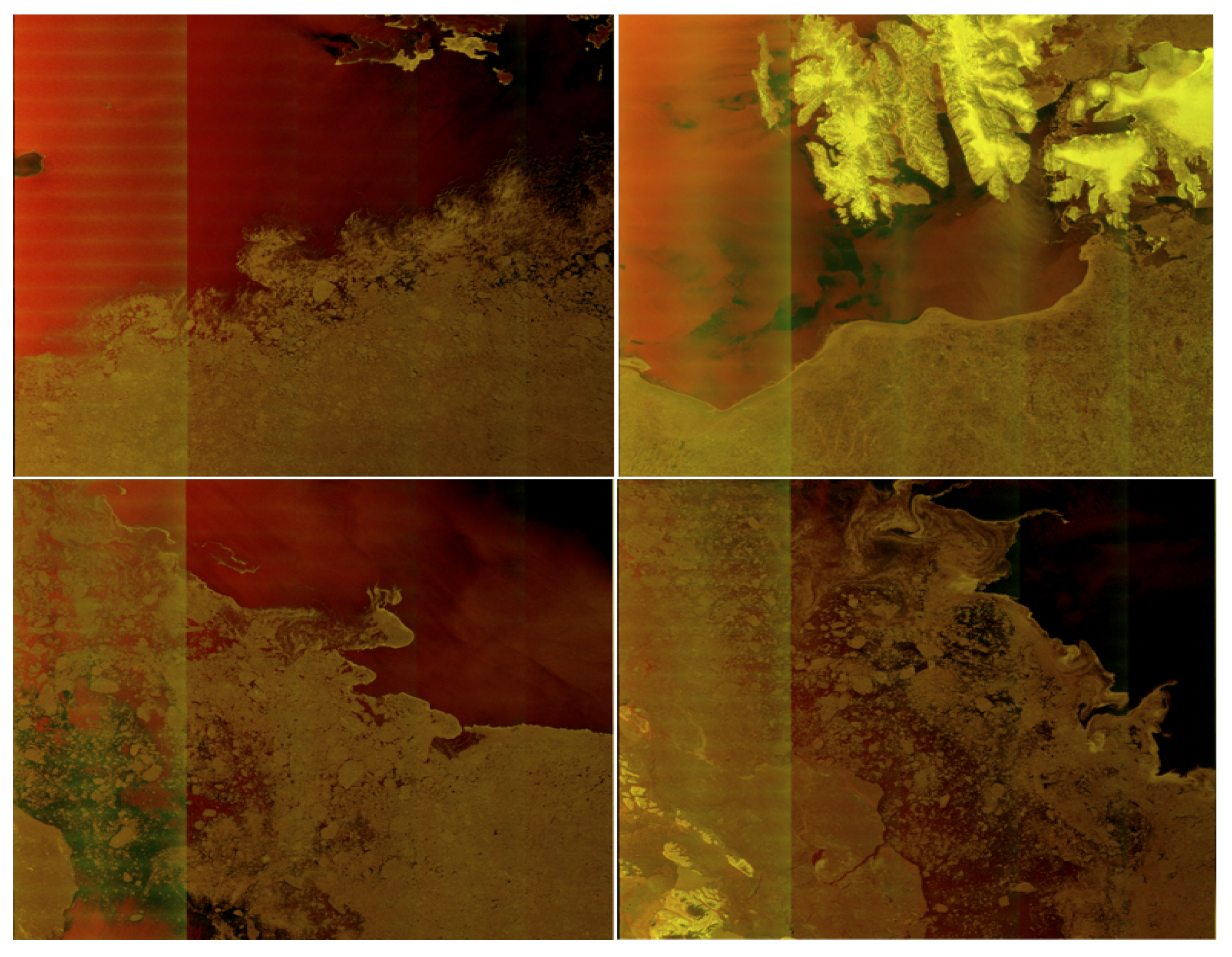
To test the deep CNN models for sea ice classification, we created an annotated dataset building on the work of Lohse et al. [56]. This is based on 31 Sentinel-1A Extended Wide (EW) Level-1 Ground Range Detected (GRD) scenes, with a spatial resolution of 40 m × 40 m, that were acquired north of the Svalbard archipelago in winter months between September and March during the period 2015–2018. Four sample images from our dataset are shown in Figure 3. Our dataset can be accessed from the provided link https://dataverse.no/dataset.xhtml?persistentId=doi:10.18710/QAYI4O (accessed on 1 March 2021). The images were pre-processed by applying a thermal noise removal algorithm in the European Space Agency (ESA) Sentinel Application Platform (SNAP) software [57], calibrated using the ${\sigma }_0$ look-up table, and multi-looked using a $3\times 3$ boxcar filter. After conversion to dB scale, the images were clipped and scaled linearly in the range [0, 1], considering the dual-polarization intensity channels individually, and including a third input-channel representing the incident angle. The range for the co-polarization (HH) is −30 to 0 dB, for the cross-polarization (HV) it is −35 to −5 dB, and for the incidence angle 19 to 46 degrees. A set of polygons representing homogeneous sea ice types was subsequently manually annotated with labels for those types, taking into account additional information from co-located and nearly temporally coincident optical image data from Sentinel-2. Patches were then extracted from these polygons for 5 different classes representing: Water (including ice-free water (windy), ice-free water (calm), and open water in leads), Brash/Pancake Ice, Young Ice, Level First-Year Ice, and Deformed Ice (including both first-year and multi-year ice). The stride between patches was 10 pixels. In

Table 1. Number of samples for different classes namely open water/leads with water, brash/pancake ice, young ice (YI), level first year ice (FYI), and old/deformed ice.

Codes	Classes	32 × 32
02	Open Water/Leads with Water	9318
01–02	Brash/Pancake Ice	159
83	Young Ice (YI)	202
86–89	Level First-Year Ice (FYI)	213
95	Old/Deformed Ice	9137

, we provide the code values for the ice types related to the stage of development (ice age), as defined by the SIGRID-3 vector archive format for sea ice georeferenced information and data ([58]), the class names, and the number of samples for each class for a patch size of 32 × 32. It is worth noticing that we have an imbalanced dataset, where the number of samples for each class has considerable variation. This is a result of the effort we made to accurately annotate the polygons, and hence the number of polygons was small and not representing all classes equally.

For binary Water/Ice classification, we grouped the samples into two classes, namely Water and Ice. Our motivation for performing binary classification is to investigate if deep models can distinguish between sea ice and water, which would subsequently allow for quantitative sea ice concentration mapping. The number of samples of water and ice for different patch sizes are shown in

Table 2. Number of samples for sea/ice classification in different patch sizes. For example, the total number of patches are 19,029 in case of patch size equal to 32 × 32.

Patch Size	Total	Ice	Sea
10 × 10	22,999	12,723	10,276
20 × 20	21,020	11,301	9719
32 × 32	19,029	9711	9318
36 × 36	18,469	9255	9214
46 × 46	17,237	8255	8982

, and there is not a class imbalance problem in this case. For all the tests, 80 percent of the dataset was used for training and 20 percent for validation.

We would like to mention that in the inference experiment, we used completely different images. These were another 4 scenes from north of Svalbard, and 8 scenes from Danmarkshavn, East Greenland that were each collected during separate months in 2018.

4.2. Model Accuracies

4.2.1. Patch Channels and Sizes

In the first study case, we report the validation accuracy by considering three different channel compositions. We calculate the validation accuracy for a patch by checking if the predicted class is the same as the true class, and by comparing the index of the highest scoring class in the predicted vector with the index of the actual class in the ground truth vector. It is interesting to use the HH polarization alone since it generally has a stronger signal and is less affected by additive noise. However, the HV polarization is more sensitive to ice types during freezing conditions and provides information about the different classes [56]. Furthermore, it is well-known that the radar backscatter from sea ice is dependent on the incidence angle, with lower incidence angles appearing brighter [56]. In order to study the importance of this effect for different classes, we included the incidence angle as a separate input channel. Hence, we consider three alternatives. First, we extracted one-channel patches using only the HH polarization. Secondly, we extracted two-channel patches, with both the HH and HV polarizations as inputs. Finally, we extracted three-channel patches by considering the HH and HV channels, plus the incidence angle. The results for these channel compositions are summarized in

Table 3. Validation accuracy of ad hoc CNN for different Patch compositions including HH, HH-HV, and HH-HV-incidence angle. The patch size is equal to 32 × 32 with spatial resolution 1440 m${}^2$.

	HH	HH, HV	HH, HV, Incidence Angle
Validation Accuracy	88.4%	98.2%	98.4%

for the ad hoc CNN, using a patch size of 32 × 32. As can be seen, the composition of the input patches affects performance of the model, with a large improvement due to adding the HV channel to the HH, and another small improvement by adding the incidence angle. The improvement of adding the incidence angle is surprisingly small. However, based on the validation results for the ad hoc CNN, we will use all three channels in our next experiments.

Next, we studied the effect of using different patch sizes for the three-channel case. We consider the ad hoc architecture and input patch sizes of 10 × 10, 20 × 20, 32 × 32, 36 × 36 and 46 × 46, respectively. The validation results in

Table 4. Validation accuracy using ad hoc CNN with different patch sizes including 10 × 10, 20 × 20, 32 × 32, 36 × 36, and 46 × 46.

	10 × 10	20 × 20	32 × 32	36 × 36	46 × 46
Validation Accuracy	95.54%	97.49 %	98.53 %	98.75 %	99.09%
Spatial Resolution (meter)	400	800	1280	1440	1840

show that the accuracy improves with the increase in the patch size. However, this improvement comes at the cost of a lower spatial resolution as larger patches cover wider areas of the surface. Note that for S1 EW GRD images each pixel covers $40\times 40$ meters on the Earth surface and, for example, a patch size equal to 46 × 46 covers a 1840 × 1840 square meters area. This patch will be classified as water if the majority of the pixels represent water and would be a problem at ice edges as classification based on larger patches would lead to coarser or non-smooth edges. Hence, there is a trade-off between accuracy and resolution. We used smaller patch sizes in our other experiments.

4.2.2. Different Training Strategies

In this section, we study the performance of the VGG-16 architecture for sea ice classification from SAR images under different training strategies. These strategies include: (a) training the network by transfer learning, where the pre-trained network is trained on the ImageNet dataset, (b) training the network from scratch, (c) training the network from scratch, with an augmented dataset, (d) training the modified VGG-16 network from scratch considering the augmented dataset with a patch sizes equal to 32 × 32, and (e) similar to (d) with a patch size of 20 × 20. Transfer learning and data augmentation are well-known learning strategies that have been successfully applied in computer vision applications. The image formation process for SAR images is fundamentally different from optical images, and our objective here is to understand if these techniques are also suitable for the sea ice classification task using SAR data. For training our model, we consider the learning rate equal to 0.001 and batch size equal to 20.

The number of convolutional layers of the VGG-16 network is different from the ad hoc network. Therefore, the extracted features are different in these architectures, and presumably also their classification performances. We present the classification results related to the VGG-16 network with different training approaches in

Table 5. The comparison of the validation accuracy of different models: VGG-16 transfer learning, VGG-16 trained from scratch, VGG-16 trained from scratch with augmentation, VGG-16 modified with augmentation considering two different pixel resolutions.

Training Strategies	Validation Accuracy	Resolution in Pixels	Resolution in Meters
VGG-16 transfer learning	97.9	32 × 32	1280
VGG-16 trained from scratch	99.5%	32 × 32	1280
VGG-16 trained from scratch with augmentation	99.79%	32 × 32	1280
VGG-16 Modified + augmentation	99.89%	32 × 32	1280
VGG-16 Modified + augmentation	99.30%	20 × 20	800

. As can be seen, when the network is trained by transfer learning, the validation accuracy is equal to 97.9%, whereas when the same network is trained from scratch, the accuracy is 99.5%. Figure 4 shows the training and validation losses for these two cases, transfer learning in the left panel and ’from scratch’ learning in right, respectively. We note that the validation losses in both panels show increasing trends after the point where the training losses indicate conversion, meaning these networks suffer from overfitting.

The issue of overfitting is often related to sparse training data, and can be remedied by extending the training set using data augmentation. We demonstrate this for the strategy of training the network from scratch, since as shown in Table 5 it has the best performance. We train the VGG-16 network from scratch with the augmented data according to the augmentation strategy described above. Figure 5 presents the corresponding training and validation loss curves, and, as can be noted, both the validation and training losses are decreasing, hence, showing better generalization capabilities. Table 5 shows that data augmentation also improves the classification results. In fact, we achieve a validation accuracy equal to 99.79%, which is remarkably good.

We also report the validation accuracies of the modified VGG-16 network trained from scratch using the augmented dataset considering two different patch sizes, namely 32 × 32 and 20 × 20. We remind the reader that this architecture is designed to have a reduced number of maxpooling layers, and hence would allow for better texture preservation and smaller input patch sizes. Table 5 also displays the validation accuracies for these models, and as can be noted, the modified VGG-16 networks achieves very high validation accuracies. We also perform a comparison with three other reference models to show the stability and robustness of our modified VGG-16 model for sea ice classification. These reference models are MobileNetV2 [59], RestNet50 [60], and DenseNet121 [45]. The performance of our model in comparison with these reference models is presented in Figure 6 in the form of validation accuracy over time. As can be seen, our model presents higher and consistent validation accuracy.

Based on these experimental analyses, we observe that the modified VGG-16 network trained from scratch with the augmented data provides the highest accuracies. This leads us to conclude that in the case of sea ice classification from SAR data, training the network from scratch with an augmented dataset enables better adjustment and learning of the sea ice characteristics. Transfer learning, with pre-training on ImageNet data, which is fundamentally different from SAR data, does not allow the same adaptation to the data. Moreover, by reducing the number of maxpooling layers, the network better preserves the structure of the data and shows improved performance.

4.3. Inference Results

In order to assess the robustness of the proposed approaches, we investigated the classification results for four new SAR scenes from north of Svalbard, i.e., scenes that are not part of the training data, by presenting the results as qualitative ice versus water maps. To this aim, we set up the inference experiment in a patch-wise manner, where the images are partitioned into non-overlapping patches, and the classification is performed on the entire patches.

Figure 7 shows the four input images from north of Svalbard in the first row. In the same figure, the patch-wise results of the ad hoc CNN are presented in the second row, the results of the VGG-16 model trained with transfer learning are presented in the third row, the results of the VGG-16 model retrained from scratch without the augmented data are presented in the fourth row, the results of the VGG-16 model retrained from scratch with the augmented data are presented in the fifth row, and the results of the modified VGG-16 model trained from scratch with augmented data are presented in the sixth row. Areas consisting of water are annotated in blue and areas consisting of sea ice are annotating in white. For better visualization, we applied a land mask to detect land areas, and the black regions in the images represent land areas. We zoom in on parts of some images to highlight specific details. The classification results obtained with ad hoc CNN (second row) are not satisfactory. The classified images are severely affected by the banding additive noise pattern, as can be clearly seen in columns two and three. The VGG-16 trained with transfer learning (third row) does not classify sea ice areas properly. In fact, open water and newly formed sea ice often have lower radar backscatter values in HV than in HH channels.These cross-polarization values are closer to the noise floor and therefore often have a lower signal-to-noise ratio producing artifacts due to different noise patterns. It can lead to problems during the interpretation of sea ice maps because the added intensity corrupts the true back scattered signal of the sea ice region.

In Figure 7, The VGG-16 retrained from scratch without using the augmented data (fourth row) is better than ad hoc CNN and VGG-16 trained with transfer learning. However, there are still some misclassifications, as can be seen in the first column. The second last row presents the results obtained with the VGG-16 model retrained from scratch with the augmented data. The last row presents the results obtained with the modified VGG-16 retrained from scratch with the augmented data. For the modified VGG-16 model, we reduced the number of maxpooling layers. In this case, the noise seems to be quite well handled, as can be seen in the second column of the last row. However, there is still some noise effects in the third column. Hence, it is worth noticing how the results are affected by the additive noise, which can be seen in the original images (row one) as distinct bands marking the different sub-swaths, and in particular the case when the ad hoc CNN and VGG-16 with transfer learning are considered. Nevertheless, the results obtained by using VGG-16 trained from scratch appear to be more robust against the noise. From this experimental analysis, we conclude that the patch-wise classification results seem to be better when the training data obtained from data augmentation is used to train the VGG-16 model from scratch. The improvement is evident in the last row of Figure 7.

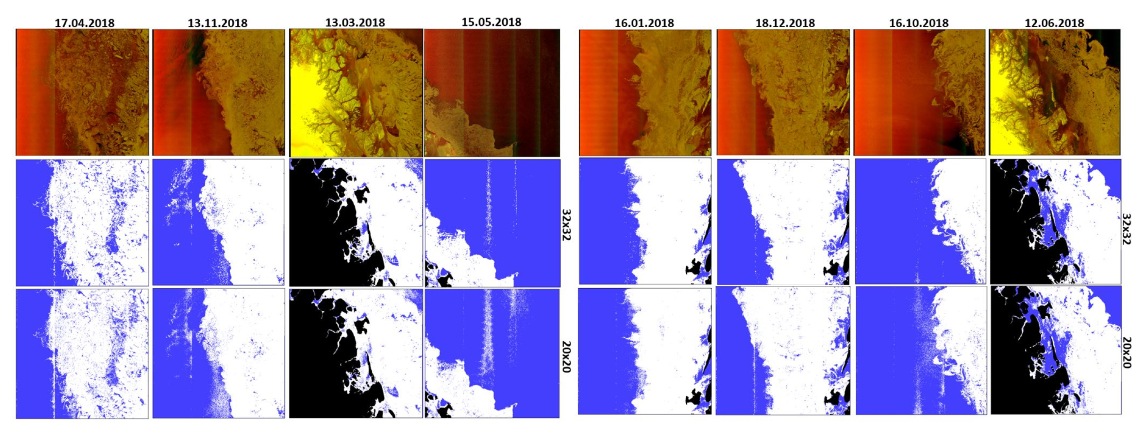
To further show the generalization performance of the CNN models for ice versus water classification, we also tested the models on images acquired from a different Arctic region, the area offshore of Danmarkshavn, East Greenland (76°46′ N, 18°40′ W). Here the Norwegian Meteorological Institute provided vector polygon data representing manually interpreted sea ice areas for the SAR data [61], which consisted of eight images, corresponding to eight different months of the year. These including both the freezing and melting seasons, and were then analyzed with the trained architectures. Figure 8 displays the classification results corresponding to the modified VGG network, trained from scratch with data augmentation, using patch sizes of 32 × 32 and 20 × 20.

As can be seen, the overall performance is good. It is also noticed that the results obtained with patch size equal to 32 × 32 are better than the results obtained with patch size equal to 20 × 20. The larger patch-size seems to be less affected by the noise and therefore we conclude that a patch size equal to 32 × 32 is a better choice for Sentinel-1 SAR images corrupted by additive noise. Overall, our experimental analysis shows that the VGG-16, when trained from scratch with augmented data, presents very good classification results when trained in a supervised fashion.

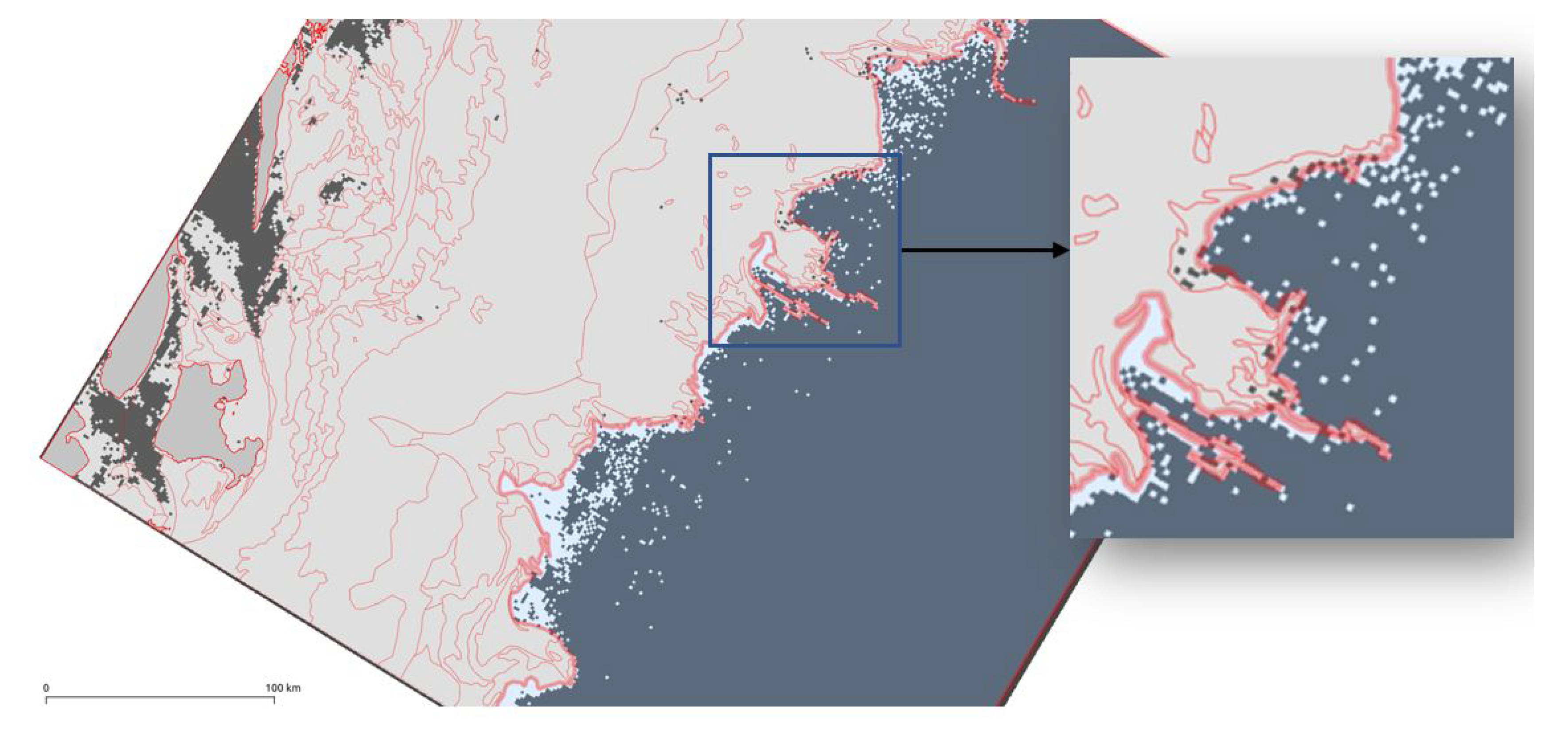
To better characterize the quality of the sea ice classification, it is important to distinguish between ice edges and water. Therefore, we also present the performance of our proposed method considering the ice edges of 16 January 2018 as depicted in Figure 9. For this purpose, we overlay the ice polygons (Norwegian Meteorological Institute [61]) from the Danmarkshavn region over the geo-referenced classified image from our method. Overestimation means predicting a larger sea ice area than the manually labelled cover area. Underestimation means predicting a smaller sea ice area than the manually labelled cover area. As can be seen, our proposed method performs effectively to separate ice edges from the water, although there remains some minor overestimation of the sea ice extent in some areas which is preferable to underestimating. However misclassification still occurs in interior areas of the ice pack where there is low backscatter from both cross- and co-polarization such as for areas of level, undeformed landfast ice close to the Greenland coast. An assessment of the accuracy of the ice edge, based on the Integrated Ice Edge Error (IIEE) metric [62], was performed on this example against a selection of other data sources. In

Table 6. Area differences and IIEE scores for the 16 January 2018 VGG-16 results, (Figure 9) against 4 different sea ice data products: manual analysis [61], Norwegian Ice Chart, OSI SAF SIC [64], and University of Bremen AMSR2 SIC [63].

Products	Overestimation km${}^2$	Underestimation km${}^2$	IIEE km${}^2$
Manual Analysis [61]	3766	4646	8412
Norwegian Ice Chart	1522	6632	8155
OSI SAF SIC [64]	10,797	5482	16,279
Bremen AMSR2 SIC [63]	2637	5966	8604

it can be seen that the contribution to the error from classifying ice as water (under-representing the ice) is consistent with all the products (4646 to 6632 km²) that are compared, as these have fairly good agreement on the presence of landfast ice. There is also a similar level of error against products with accurate ice edges (1522 to 3766 km²) such as the manually analyzed polygons introduced earlier [61], the Norwegian Ice Chart from the Norwegian Meteorological Institute (https://cryo.met.no/en/latest-ice-charts, accessed on 1 March 2021) which is the routine operational analysis produced by an ice analyst, and the sea ice concentration (SIC) produced by the University of Bremen from Advanced Microwave Scanning Radiometer 2 (AMSR2) data [63]. Products based on low resolution passive microwave radiometry, for example the EUMETSAT Satellite Application Facility on Ocean and Sea Ice (OSI SAF) SIC that uses Special Sensor Microwave Imager/Sounder (SSMIS) [64], are less capable of resolving the ice edge, and here there is a far greater contribution to the IIEE (10,797 km²) because the SAR classification correctly identifies sea ice.

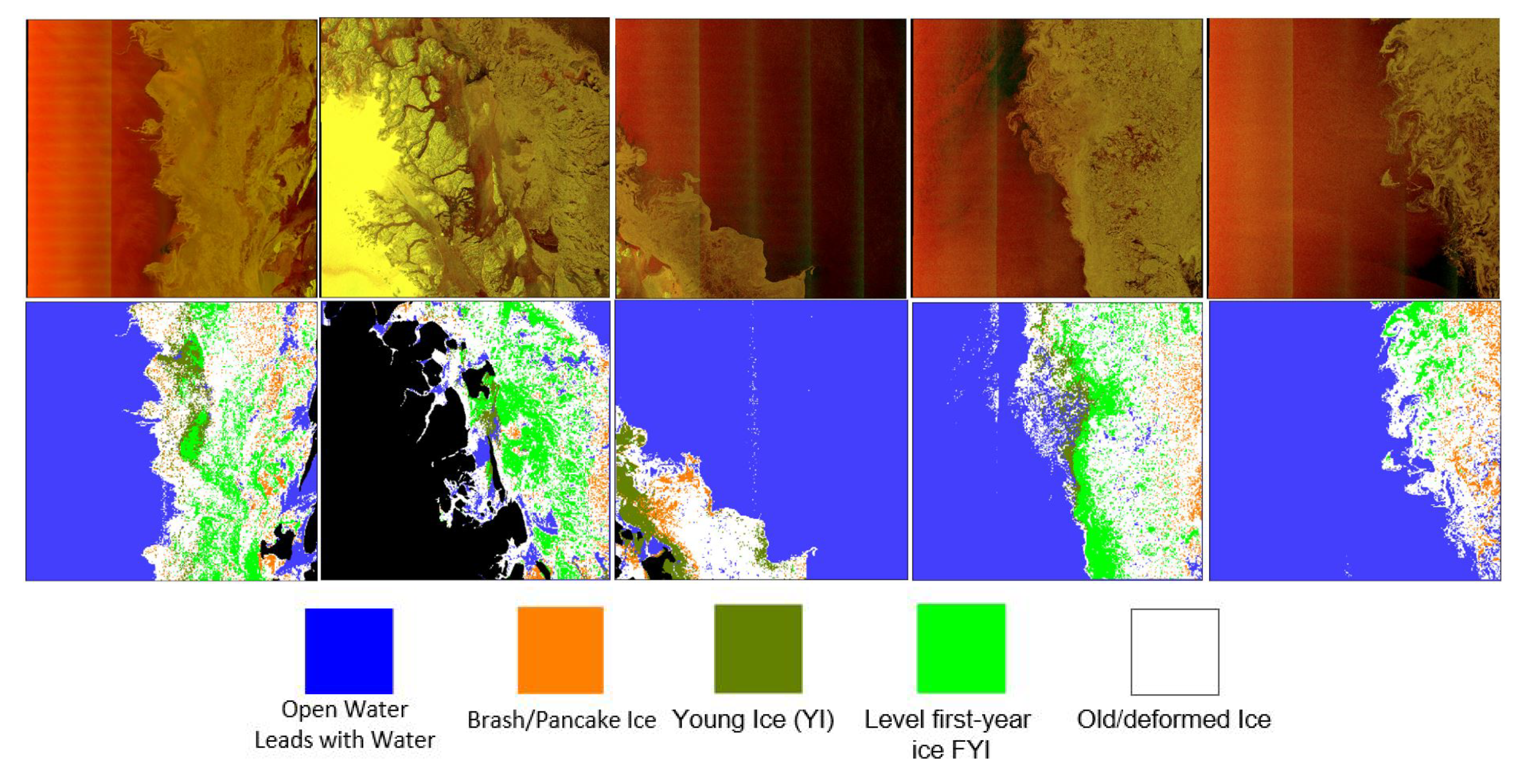
We have also extended our experimental analysis to multi-class sea ice type classification considering five images from the Danmarkshavn region. The results are depicted in Figure 10. In this classification experiment, we used the modified VGG-16 model trained from scratch with the dataset from north of Svalbard as shown Table 1.

We would like to emphasize that our dataset is scarce and unbalanced, with an unequal number samples from the ice types. This is affecting the classification performance, and the results presented in Figure 10 are slightly biased toward ice types where we have more samples than others. The effect of the imbalance data can be seen in Figure 10, where brash/pancake ice is detected in the right-hand side of the right-most image, which apparently is a dense ice area. In general, brash/pancake ice is located at the edges towards open water. Despite this problem, the results indicate that the VGG-16 trained from scratch shows promising performance in distinguishing different ice types as well as binary ice versus water classification.

We also present the inference result obtained considering only the HH channel. In Figure 11, the left column shows the input SAR image and the right column shows the inference results. As can be seen, the inference result lacks coherency to distinguish sea ice from water. Therefore, both the HV channel and incident angle contribute to the process of properly training the model.

5. Conclusions

In this work, we explored the potential of different CNN models for sea ice classification. We tested and assessed the results both qualitatively and quantitatively. The results showed that these complex architectures (such as those based on the VGG network) typically obtain promising classification results. Moreover, we evaluated the value of data augmentation, and found that even if the quantitative performance improvement was only minor, the data extension technique seemingly can prevent over-fitting caused by a scarce training dataset. We also assessed the robustness of the trained CNN models when applied to SAR scenes collected at different spatial locations and times. Even though our analysis is limited to only a few scenes, our findings are positive and show that the models have good potential. The computational processing to obtain the inference result for a single high resolution SAR image requires a few minutes on a typical desktop computer. We also found that the additive system noise in the SAR imagery is a challenging problem to obtaining refined sea ice maps. Both the computational requirements and the additive system noise are important issues for the operational use of SAR data for sea ice classification.

We also trained our models to perform multi-class classification. In this preliminary study, we had a scarce and unbalanced dataset, which obviously affected the output, but the analysis still showed promise. This motivates us to carry out our research in this direction. In our investigation we performed patch-wise classification which degrades the spatial resolution. Future work will address a pixel-wise setup. However, the pixel-wise set-up will be driven by more computational overhead. Therefore, our future work will also focus on transforming the current architecture to process the input data quickly. For this purpose, we will replace the fully connected layers by convolution layers based on the work of Sermanet et al. [65]. To reduce the impact of noise on sea ice classification, we would include the nominal noise profiles as a feature directly into the model. Finally, we emphasize that the scarcity of reliable and balanced sea ice training and validation datasets is a severe problem for these complex CNN architectures and needs full attention from the sea ice community. In future work, we will develop semi-supervised learning methods to partly remedy this issue.