Article

Optimized Deep Learning Model as a Basis for Fast UAV Mapping of Weed Species in Winter Wheat Crops

1
Leibniz Institute for Agricultural Engineering and Bioeconomy e.V., Potsdam-Bornim, Max-Eyth-Allee 100, 14469 Potsdam, Germany
2
Institute of Computer Science, University of Potsdam, August-Bebel-Str. 89, 14482 Potsdam, Germany
3
Julius Kühn-Institut, Institute for Plant Protection in Field Crops and Grassland, Messeweg 11–12, 38104 Braunschweig, Germany
*
Author to whom correspondence should be addressed.
Remote Sens. 2021, 13(9), 1704; https://doi.org/10.3390/rs13091704
Submission received: 7 March 2021 / Revised: 9 April 2021 / Accepted: 25 April 2021 / Published: 28 April 2021
(This article belongs to the Special Issue UAV Photogrammetry for Environmental Monitoring)

Abstract

:
Weed maps should be available quickly, reliably, and with high detail to be useful for site-specific management in crop protection and to promote more sustainable agriculture by reducing pesticide use. Here, the optimization of a deep residual convolutional neural network (ResNet-18) for the classification of weed and crop plants in UAV imagery is proposed. The target was to reach sufficient performance on an embedded system by maintaining the same features of the ResNet-18 model as a basis for fast UAV mapping. This would enable online recognition and subsequent mapping of weeds during UAV flying operation. Optimization was achieved mainly by avoiding redundant computations that arise when a classification model is applied on overlapping tiles in a larger input image. The model was trained and tested with imagery obtained from a UAV flight campaign at low altitude over a winter wheat field, and classification was performed on species level with the weed species Matricaria chamomilla L., Papaver rhoeas L., Veronica hederifolia L., and Viola arvensis ssp. arvensis observed in that field. The ResNet-18 model with the optimized image-level prediction pipeline reached a performance of 2.2 frames per second with an NVIDIA Jetson AGX Xavier on the full resolution UAV image, which would amount to about 1.78 ha h−1 area output for continuous field mapping. The overall accuracy for determining crop, soil, and weed species was 94%. There were some limitations in the detection of species unknown to the model. When shifting from 16-bit to 32-bit model precision, no improvement in classification accuracy was observed, but a strong decline in speed performance, especially when a higher number of filters was used in the ResNet-18 model. Future work should be directed towards the integration of the mapping process on UAV platforms, guiding UAVs autonomously for mapping purpose, and ensuring the transferability of the models to other crop fields.

Graphical Abstract

1. Introduction

Today, artificial intelligence renovates the extraction of information from very-high-resolution remote sensing data (VHR) with neural networks established in deep learning architectures tailored specifically for the needs of image data. This enables object recognition and classification in much higher detail and accuracy than before, and combined with imagery obtained from unmanned aerial vehicle (UAV), a smarter monitoring of agricultural lands is thinkable. Applied to the right scenario, this might pave the way for a more sustainable agriculture [1].
One such application would be site-specific weed management (SSWM). Conventionally, pesticides are supplied with dosage instructions that are calculated uniformly on a “per hectare” basis for the entire field. The target is in this case the area within the field and not the weed as such. For SSWM, in contrast, the target is directed to the weed plants. Weed plants normally exhibit an aggregated pattern in patches over the field [2,3]. Thus, SSWM can reduce the amount of unused herbicide that reaches the ground and misses the target plants. This is consistent with government regulations and policies in the European Union aiming at considerably reducing the amount of pesticide used in agriculture by 2030 [4]. For SSWM, it is important to delineate the location and the size of weed patches in the field. To achieve this, sensors for automatic weed detection are needed to replace visual weed scouting in the field. Depending on the way in which weeds are recognized in the field, two approaches for SSWM can be outlined—the online and the offline approach [5,6]. In case of the online approach, the determination of weeds and the spraying action is performed in one operation step. For example, a tractor may be equipped with a sensor capable of detecting the weed cover and, then, regulates an implement that controls the spray liquid ad hoc. In the case of the offline approach, weed detection and spraying are done in two separate operation steps. Weed maps are first generated and translated to prescription maps, which will then be passed to variable rate herbicide sprayers to vary application rates according to the weed spatial variability. Thus, the spraying amount can decrease if the coverage value or the number of weed plants decreases and vice versa while driving over the field. The spatial accuracy of herbicide application has become quite reliable with the commercial spraying technology available for SSWM [7].
In recent years, small UAV platforms have become increasingly popular in precision agriculture, because they provide flexible and cost-effective monitoring of fields, offer small ground sample distances, enable on-demand collection, and provide information to the farmer quickly [8,9,10]. UAVs can be piloted towards altitudes from which images can be captured that contain details to identify even subtle structures of individual plants in crop fields with non-sophisticated camera systems such as snapshot RGB systems. This allows information to be extracted from the images that can be used to arbitrarily distinguish not only between crops and weeds, but also what type of weeds are present in a particular location of the field [11]. UAV technology would offer tremendous advantages for SSWM. Detailed weed maps from UAV imagery can be generated to accurately delineate weed patterns and patches in the field [12]. The capability of differentiating among the weed species would further enable selective herbicide application [13]. More accurate and detailed weed maps would also improve the understanding about weed concurrence and competition for analyzing and predicting the propagation mechanisms of weeds and improve the accuracy of spatio-temporal models of weed populations for agronomists and ecologists [14,15]. As part of a smarter agriculture, online weed assessment by UAV could guide weed robots more efficiently across the field [16], or UAVs extended with spraying equipment could control selected areas of the field directly from the air only where needed [17,18].
There have been a number of attempts to generate site-specific weed maps in the past using UAV remote sensing. Since the spectral characteristics of crop and weed plants can be highly similar in the early season, the use of object characteristics of plants and plant associations has been seen to be highly effective in improving the results for weed mapping [19]. Specifically, for the general crop–weed differentiation, many studies propose a multi-step classification approach using an object-based image analysis methodology (OBIA). Peña et al. [20] suggested an OBIA procedure for weed classification of UAV imagery using a combination of several contextual, hierarchical, and object-based image features in a three-step algorithm. This included the identification of crop rows on their linear pattern, the discrimination between crop and weed plants, and a subsequent gridding for generating the weed map. They concluded that UAV imagery and OBIA in combination are a favorable technology over airborne and satellite remote sensing to produce crop-weed maps for calculating herbicide requirements and planning weed control application in advance. In a later study, they were able to obtain good discrimination results between plants and weeds even within plant rows by further refining the OBIA model with a random forest classifier incorporating 3D surface information from UAV photogrammetry [21].
For differentiating individual plant details to identify the type of weed species, UAVs need to collect the imagery from altitudes nearly below 10 m [11]. Yet, to map entire fields with such a small ground sample distance would require lots of aerial images, especially if image overlap is needed for photogrammetry. Thus, one problem with UAV imagery from a low altitude would be the sheer volume of image data, which would hinder rapid weed mapping, because it is impractical in terms of data storage, handling, and further processing with photogrammetry and OBIA. A more economical and flexible approach would be an image classifier capable of automatically and quickly identifying weeds from UAV images. This would allow weed mapping directly from a UAV platform as it flies over the field, while image recognition is embedded in a single computer aboard the platform that analyzes the images online. This way only the necessary information for weed mapping can be stored away or transferred to a ground station, such as the classification image, position, and type of the weed plants from post classification or, even more abstractly, summary statistics over the complete image, e.g., overall coverage of weeds with regard to species level in that image.
With some success, global features of plant morphology such as convexity, contour, or moments have been used in image classifiers to identify individual plant species directly from images [22,23,24,25]. Yet, these approaches begin to fail if cluttered imagery, such as UAV images from crop fields, is used. More recently, the use of local invariant features within the framework of bag-of-visual words [26] has been tested successfully for identifying weed species in cluttered field imagery [11,27]. This type of classifier only failed if weed species were very similar in their appearance [11]. Even more promising seems the use of convolutional neural networks for identifying weed plants, specifically within a deep learning framework [28]. One benefit of deep convolutional neural networks (DCNN) is that they learn the feature filters needed to extract the relevant information from the images directly in one process within the training network using convolutional layer structures. Beginning with LeNet-5 [29], proposed in 1998 using a rather slick design with two convolutional layers and three fully connected layers with about 60,000 parameters to be fitted, the architectures became quickly deeper with the growing capabilities of modern computing hardware. Inception-V3 and ResNet-50, proposed in 2015, hold over 20 million parameters [30,31]. To train and use them optimally, more and more specialized designs became necessary. In case of the deep residual networks (ResNets), residual blocks became popularized as key features that enable shortcut connections in the architecture, which allows more efficient training of deeper DCNNs. This ability has led to a breakthrough in classification accuracy in major image recognition benchmarks such as ImageNet [32].
For weed image classification based on DCNNs, Dyrmann et al., [33] proposed an own DCNN structure and trained it from scratch with segmented images from different sources of RGB images. They achieved moderate to high classification accuracies for 22 different weed species. A. dos Santos Ferreira et al. [34] tested different machine learning approaches, e.g., support vector machines, Adaboost, random forests, and DCNN, for classifying UAV images obtained from soybean crops into soil, soybean, grass, and broadleaf classes. Among the tested approaches, the best results were obtained for a DCNN based on an AlexNet architecture [28]. They concluded that one advantage of DCNNs is their independence in the choice of an appropriate feature extractor. More recently, Peteintos et al. [35] tested three different DCNN architectures, including VGG16 [36], Inception, and ResNet-50, for the classification of weeds in maize, sunflower, and potato crops with images taken from a ground-based vehicle, in which the VGG16 was outperformed by the other two DCNNs. They also concluded that data sets for weed classification by DCNNs needs to be more robust, usable, and diverse. Weed classification was also achieved by segmentation with DCNN from images. Zou et al. [37] successfully differentiated crop from weeds to estimate weed density in a marigold crop field using a modified U-Net architecture with images taken from a UAV platform in 20 m altitude.
For online mapping with UAVs, it is paramount not only to achieve high accuracy of the image classifier for weed identification, but also to optimize the predictive capabilities of the network in terms of the speed for evaluating a full-resolution UAV image captured by the camera. Most recently, research has focused on integrating DCNNs on embedded system for identifying weed online. Olsen et al. [38] successfully trained models for classifying different rangeland weed species with Interception-3 and ResNet-50 DCNN architectures and could implement the model on NVIDIA Jetson TX2 board. They theoretically achieved an inference time of 18.7 fps for evaluating resampled weed images (224 × 224 px) collected from a ground-based vehicle. Deng et al. [39] used a semantic segmentation network based on an adapted AlexNet architecture and could effectively discriminate rice and weed on an NVIDIA Jetson TX board with 4.5 FPS. This study similarly aims for optimizing a DCNN for weed identification with embedded systems for UAV imagery. In this approach, optimization was reached mainly by avoiding redundant computations that arise when a classification model is applied on overlapping tiles in a larger input image. This is similar to fully convolutional architectures used in segmentation models, but unlike those models, this approach does not require pixel-level segmentation labels at training time, which would be too inefficient. As DCNN architecture, a deep residual type ResNet-18 structure [31] was used and taught the network to recognize the most typical weed species with UAV images collected in winter wheat crops. Based on the DCNN model and its optimization, an intelligent mapping system should be aimed for that is capable of identifying and capturing weed species from a UAV platform while it is flying over the field. Here, the optimization approach in the prediction pipeline of the ResNet-18 classifier, its implementation on an embedded system, and its performance on classifying UAV images for typical weed plants in winter wheat crops are shown.

2. Materials and Methods

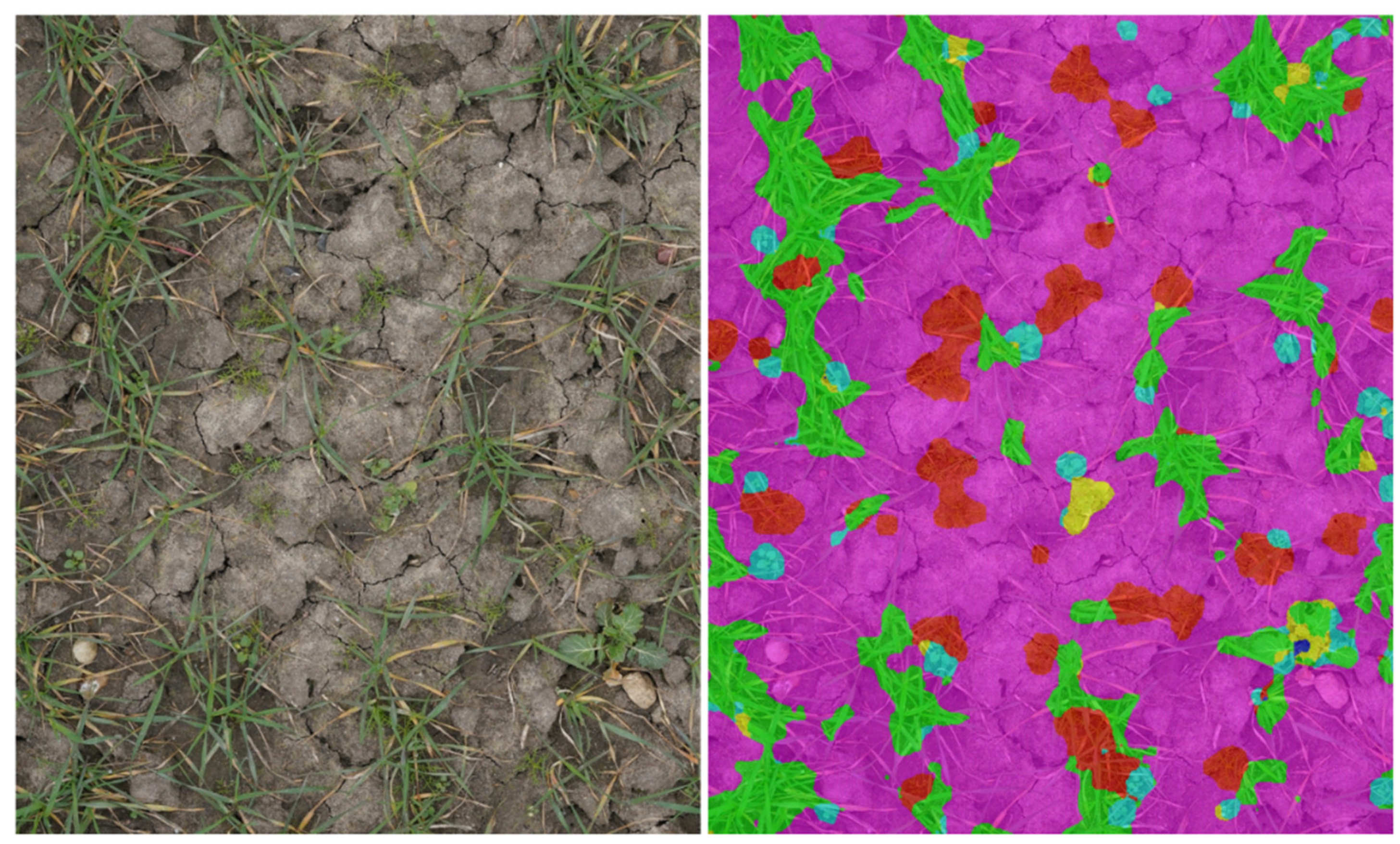
2.1. The UAV Image Data Set and Plant Annotation

The data set used in this study was originally introduced in the study of Pflanz et al. [11]. Only the essentials are repeated here. The image data was acquired during a UAV flight campaign in a wheat field (52°12′54.6″N 10°37′25.7″E, near Brunswick, Germany) conducted on 6 March 2014, when weed plants and wheat crop were abundant in the field with the wheat at development stage BBCH 23 (tillering). The flight mission was conducted between 1:00 and 3:00 p.m. in high fog and cloudy skies so that the lighting conditions were diffuse, with no direct sunlight. As UAV platform, a hexa-copter system (Hexa XL, HiSystems GmbH, Moormerland, Germany) was used, from which images could be captured at a very low altitude between 1 and 6 m over ground at 110 waypoints. The camera setup mounted below the copter consisted of a Sony NEX 5N (Sony corporation, Tokyo, Japan) with a 23.5 × 15.6 mm APS-C sensor using a lens with a fixed focal length of 60 mm (Sigma 2.8 DN, Sigma Corp., Kawasaki City, Japan). Images were shot in nadir position with a ground sample distance between 0.1 and 0.5 mm. Each image had a dimension of 4912 × 3264 px.
The field was subdivided into training and test areas. All images acquired in the training areas were used for training the model, and all images acquired in the test area were used for testing the prediction capabilities of the model. Experts examined all UAV images and annotated 24,623 plants and background by referencing the coordinates of the plants’ midpoint and their species name into an annotation database. Around each annotation coordinate, a buffer of a 201 × 201 px quadratic frame was drawn, and a sub-image or image patch was clipped to that buffer depicting the annotation item. In total, 16,500 image patches were extracted this way and used for model training.

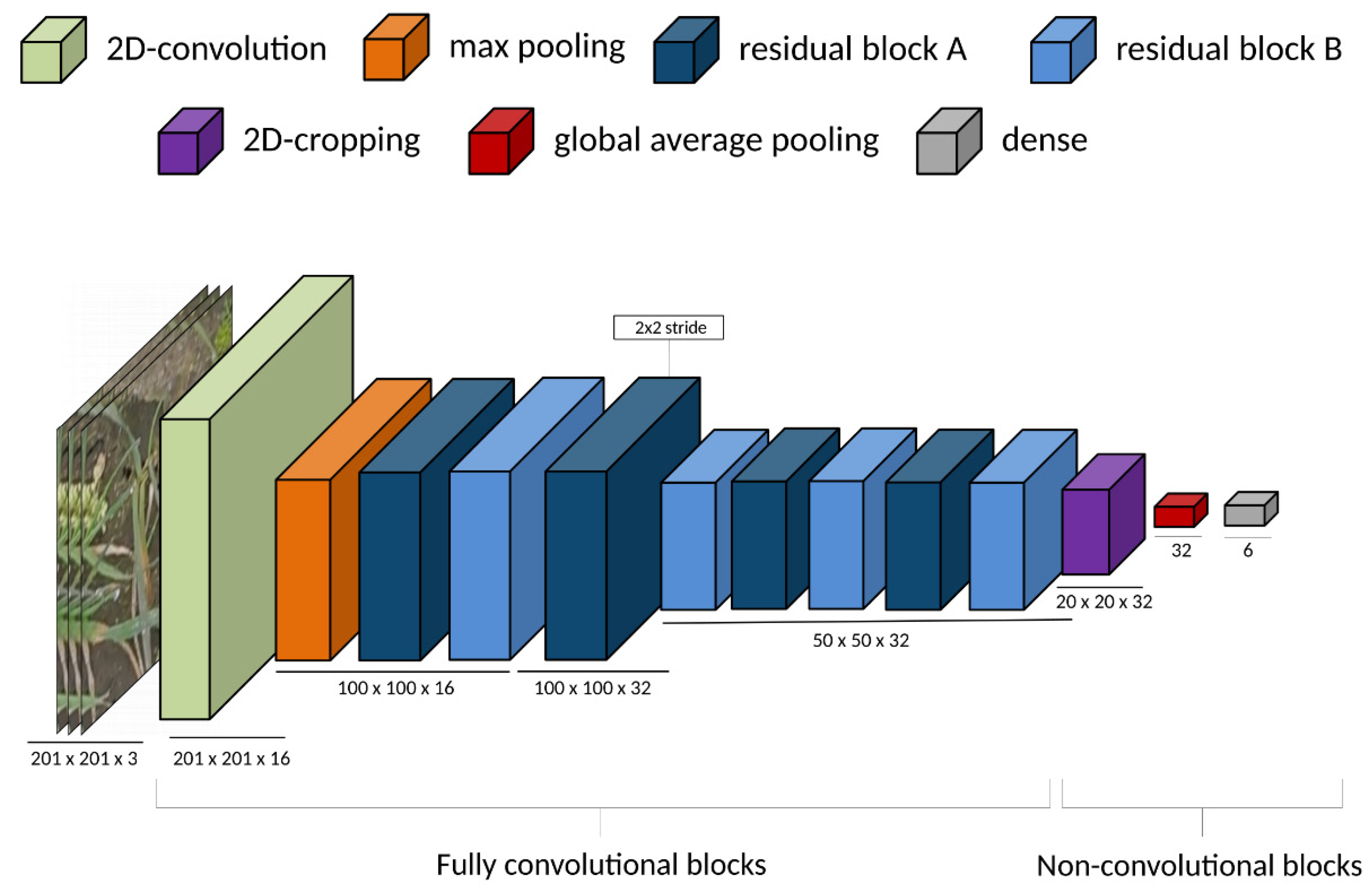
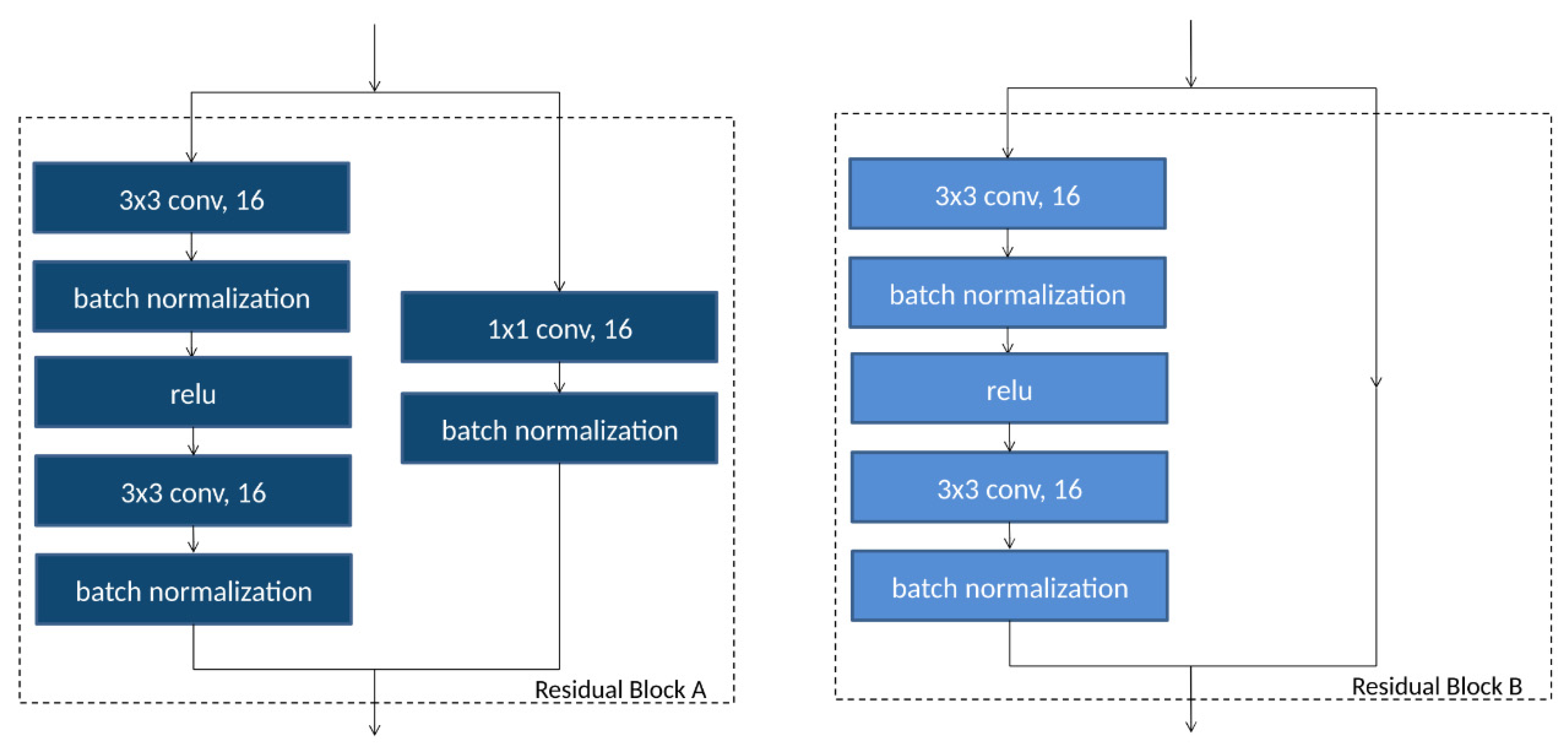
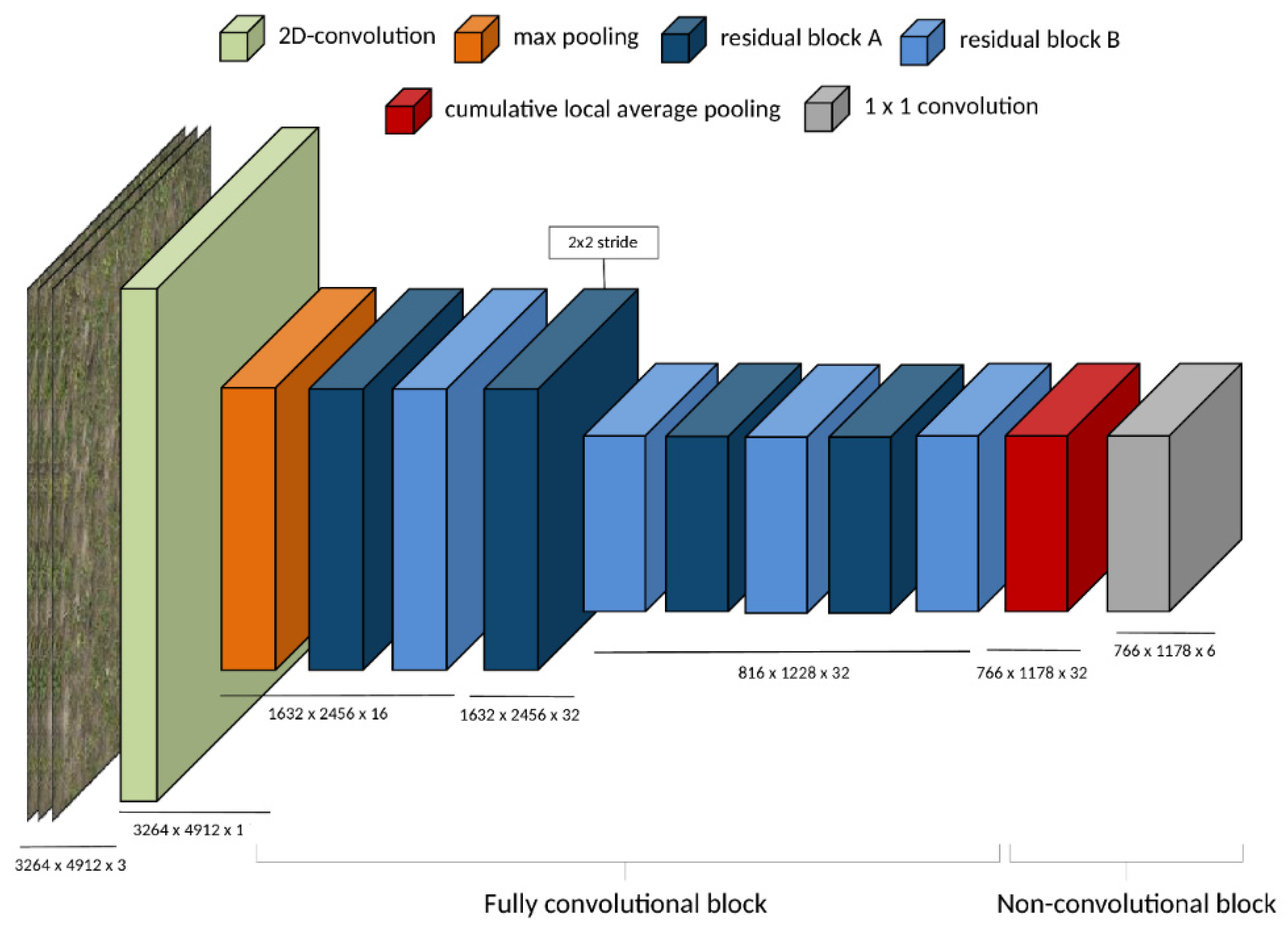
2.2. The Image Classifier Base Architecture

The core of the image classifier is a DCNN based on a residual neural network (ResNet) architecture. ResNets use so-called residual blocks that implement shortcut connections in the network architecture [31]. The stack of convolution layers within each residual block only needs to learn a residual term that refines the input of the residual block toward the desired output. This makes the DCNN easier to train, because the shortcut connections enable the direct propagation of information and gradients across multiple layers of the network, leading to better gradient flow and convergence properties of the network during calibration [40].
The specific network architecture that was used here, shown in Figure 1, is inspired by the 18-layer residual neural network architecture proposed by He et al. ([31], but deviates from this model in several aspects relevant for the optimization of computational efficiency. It incorporates two different types of residual blocks (Type A and Type B, shown in Figure 2). Type B follows the original design proposed by He et al. [31] with an identity mapping for the non-residual branch in the block, while Type A implements a modified version, where a single convolution layer is added to the non-residual branch, as in He et al. [40]. The architecture starts with a 7 × 7 convolution layer with 16 filters, followed by a stride-two 2 × 2 max pooling layer to reduce spatial resolution. Stride-two means that in the convolution layer, filters are moved at twice the spatial offset in the input as compared to the output, effectively reducing the spatial dimension of the feature map by a factor of two.
These initial layers are followed by eight residual blocks, alternating between Type A and Type B. The number of filters is 16 in the convolution layers within the first two residual blocks and 32 in all remaining convolution layers. Note that these numbers are much lower than in standard ResNet architectures to improve computational efficiency. After the first two residual blocks, the spatial dimension is again decreased by a stride-two convolution layer. All convolution layers are followed by batch normalization and nonlinear activation layers. As activation layers, rectified linear units (ReLUs) were used throughout the network as proposed by He et al. [40]. Note that the model up to and including the final residual block is fully convolutional in the sense of Long et al. [41]. However, unlike the model studied by Long et al. [40], which is a segmentation model that needs to be trained on pixel-level segmentation labels, our model is a classification model that is trained in a multiclass classification setting on 201 × 201 px inputs.
In standard ResNet architectures, the final residual block is followed by a global average-pooling layer and a dense layer for classification. In the model proposed in this study, the output of the final residual block, whose dimensions are 50 × 50 × 32, is first spatially cropped to 20 × 20 × 32 by removing the 15 neurons closest to the borders for all filters in both spatial dimensions. This spatial cropping layer is then followed by a global average-pooling layer and a dense layer for classification as in standard ResNet architectures. The rationale for the spatial cropping layer is that it removes all neurons in the output of the final residual block whose receptive field on the input would exceed the 201 × 201 px buffer once the model is turned into a fully convolutional model and applied to larger inputs. This is discussed in more detail in Section 2.3.

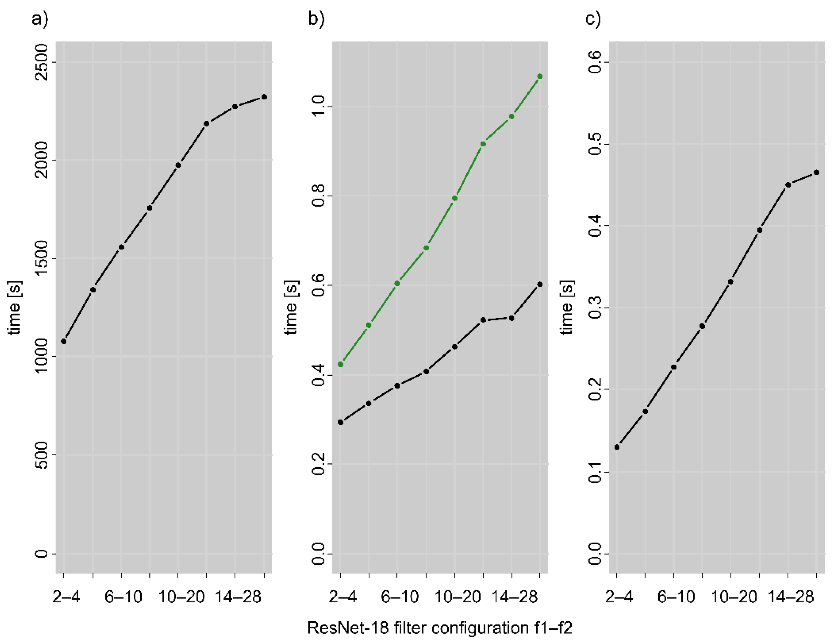
2.3. Optimizing Computational Performance for Creating Weed Maps

The trained classification model shown in Figure 2 takes as input a 201 × 201 px image patch and predicts the plant species (or bare soil) at the center of this image patch. The goal of this study is to produce high-resolution weed maps, that is, to annotate every spatial position in a large image with the plant species that is growing at that position. A straightforward way to produce such a map would be to apply the trained model to every position on a fine grid laid over the large image. However, this is computationally demanding, because the number of image patches can be very large depending on the resolution of the grid. In this study, images captured by the camera have a resolution of 3264 × 4912 px, and the aim was to classify the plant species in a four-pixel grid. This would result in 766 × 1178 = 902,348 individual classifications of 201 × 201 image patches, assuming that only patches that are fully included in the 3264 × 4912 image are used. Even for a lightweight model, this is computationally challenging, in particular if inference has to be carried out on an embedded device. Note that the image patches are strongly overlapping.
The computational performance of the proposed model was optimized by following a different approach in which the trained classification model is converted into another model that can be applied directly to the larger image, and directly outputs 766 × 1178 individual classifications for the plant species in the four-pixel grid. The trained model will be referred to as the patch-level classifier, and the converted model as the image-level classifier. The image-level classifier is designed in such a way that it is mathematically equivalent to performing the 766 × 1178 classifications with the patch-level classifier, that is, it yields exactly the same predictions as this straightforward approach. However, it is much more computationally efficient, mainly because it avoids redundant computations in the convolution layers of the patch-level classifier that would occur when applying it to strongly overlapping image patches.
To begin with the discussion of the image-level classifier, shown in Figure 3, it should be noted that the part of the patch-level classifier is fully convolutional up to and including the last residual block, that is, it can be applied directly to larger input images and then computes the corresponding larger feature maps for these larger inputs. This is much more efficient than applying the patch-level model to the many strongly overlapping image patches, as the redundant computations in the convolution layers are avoided. Applying this part of the model to a full image of size 3264 × 4912 px yields an output with a dimension of 816 × 1228 × 32 (where 816 × 1228 is the spatial dimension and 32 is the number of channels), because the two spatial pooling layers in the network jointly reduce the spatial dimension by a factor of four.
A 50 × 50 × 32 spatial patch from this 816 × 1228 × 32 output is essentially equivalent to the 50 × 50 × 32 output that would have been generated at the end of the last residual block in the original patch-level model if one had applied it to a particular 201 × 201 patch in the full image. However, the activation values in a 50 × 50 × 32 patch from the 816 × 1228 × 32 output are not exactly identical to the values one would get from the last residual block in the patch-level classifier applied to the corresponding 201 × 201 image patch. This is because the outer neurons in the 50 × 50 × 32 patch have a receptive field that covers more than 201 × 201 px in the input image. In the patch-level classifier, they would see borders that are padded with zeros, while in the image-level classifier they see pixels outside of the 201 × 201 area. However, all activations within the inner 20 × 20 spatial positions of the 50 × 50 × 32 patch are identical to the output of the 20 × 20 spatial cropping layer in the patch-level classifier, which is why the cropping layer was added to the patch-level classifier (see Section 2.2 and Figure 3). Note that there are 766 × 1178 different positions for the 50 × 50 × 32 spatial patch within the 816 × 1228 × 32 output, just as there are 766 × 1178 different positions for the 201 × 201 patch from the original image at a four-pixel grid.
To complete the image-level classifier, one needs to implement layers that mimic the operation of the last three layers (cropping, global average pooling, dense layer) in the patch-level model for each of the 766 × 1178 grid positions. The cropping and pooling part could be achieved with a standard 20 × 20 spatial average pooling layer; however, this pooling layer would account for a significant fraction of the total computational cost of inference. The problem is that pooling is carried out over strongly overlapping patches, leading again to redundant computations. An equivalent and more efficient way of implementing the pooling operation is thus to compute cumulative sums along both the x-axis and the y-axis over the entire 816 × 1228 × 32 output and subtracting the cumulative sums at the correct indices to obtain the sum over the 20 × 20 spatial patches, which can then be normalized to the average. This efficient procedure was implemented in a custom layer (called cumulative local average pooling in Figure 3). Finally, the dense layers in the patch-level model can be translated into a corresponding 1 × 1 convolution layer in the image-level model. This computes for each grid position the product between a particular 1 × 1 × 32 entry from the 766 × 1178 × 32 feature map with a 32 × 6 weight matrix to yield the six class scores, much like the dense layer in the patch-level model computes class scores from the 32 values resulting from global average pooling. The 1 × 1 convolution layer inherits the weights from the dense layer of the patch-level classifier.
To summarize, for a 3264 × 4912 px image, the image-level classifier will compute exactly the same class probabilities as a patch-level classifier moved over the image at a four-pixel grid. As there are 766 × 1178 possible positions in a four-pixel grid, the output of the image-level classifier is of size 766 × 1178 × 32. That is, it makes a prediction every four pixels (horizontally and vertically). Therefore, the output is only one fourth of the original image size. Therefore, it does make predictions for the entire image, but the predictions are at a slightly lower resolution than the original image was.
The code for the image classifier and its image-level optimization was made publicly available by the authors on GitHub repository (https://github.com/tiborboglar/FastWeedMapping, accessed on 27 April 2021).

2.4. Testing the Accuracy of the Image Classifier and Its Prediction Performance (Model Training and Testing)

Model training was based on the 201 × 201 px image patches taken from the annotation database as discussed in Section 2.1. Based on these image patches, the task was to teach the classifier to distinguish six categories: bare soil (SOIL), crop (wheat, TRZAW), and four different species of weeds observed commonly in the field, which were Matricaria chamomilla L. (MATCH), Papaver rhoeas L. (PAPRH), Veronica hederifolia L. (VERHE), and Viola arvensis ssp. arvensis (VIOAR). In the following, they are referred to by their EPPO code.
This training set was augmented by adding, for each image, copies of the image that were rotated by 90°, 180°, and 270°, and additionally for each rotation angle, copies that were mirrored left-to-right. For the training, eight different models were created. Each of these models differed in the filter configuration applied for convolution within the network. A lower number of filters was used for the shallow part of the network (Filter 1) and a higher number of filters in the deeper part of the network (Filter 2). The exact filter configuration and its naming convention are given in Table 1.
All models were trained using the same optimizer and hyperparameters, namely, the Adam optimizer with learning rate of 0.01 and without any decay [42]. The number of epochs was fixed in 100 and the batch size fixed in 32 images. A batch size of 32 is one of the most widely chosen batch sizes; typically, models are not very sensitive to batch size. The order of magnitude of the epochs needed for convergence was judged based on the behavior of the training loss and fixed at 100 to have a round number. It is not expected that the model will be sensitive to the number of epochs as long as the number is high enough. For optimization, categorical cross-entropy was used as the loss function and accuracy as metric. The trained model was implemented in Tensorflow [43] and deployed on an NVIDIA Jetson AGX Xavier embedded system (NVIDIA CORPORATE, Santa Clara, CA, USA). For prediction, the optimized procedure was used as described in Section 2.3. To further improve computational efficiency, the NVIDIA TensorRT Software Development Kit (NVIDIA CORPORATE, Santa Clara, CA, USA) was used to decrease the floating-point precision of the models from 32- to 16-bit. This procedure takes advantage of the half precision capabilities of the Volta GPU by reducing arithmetic bandwidth and thus increasing 16-bit arithmetic throughput. As halving the floating-point precision could negatively impact the prediction results, it was further demonstrated in this study if these impacts are negligible.
Each model was run five times with different randomization (seeds) of the weights. For each UAV test image, a classification map was generated this way. All classification maps were compared with 8123 annotations, which were made by experts in the UAV test images. To generate more robust outcomes for testing, the five model runs were aggregated by calculating the median over the classification results. From this, a 6 × 6 confusion matrix was calculated, which was then used to assess the metrics recall, precision, and accuracy. The weed classification in this study not only shows a binary crop-weed classification, but also discriminates between four different weed species as well as soil and winter wheat. Thus, true positive (TP), false negative (FN), and false positive (FP) values were acknowledged from a multi-class perspective. They were calculated from the 6 × 6 confusion matrices for each class separately. For example, in case of MATCH, the correct predictions of the category MATCH are called TP. FP summarizes cases in which MATCH is falsely predicted as MATCH when in fact it belongs to a different category, while FN describes cases where a different category is incorrectly predicted to be MATCH. Based on TP, FP, and FN, the following metrics were calculated:
Precision i = T P i T P i + F P i
Recall i = T P i T P i + F N i  
Overall   accuracy = i = 1 k T P i N  
The precision of a class i represents how many predicted class positives are truly real positives from the class predictions (Equation (1)). The recall of a class i represents how many predicted class positives are truly real positives from the class measurements (Equation (2)). Thus, precision focuses on the prediction, whereas recall focuses on the measurements. The overall accuracy was calculated by Equation (3) over all classes (k = 6), where N refers to the overall number of cases in the confusion matrix.
As inference time could potentially vary over different test images, measurements of inference time are given as the average time over all images in the test set. Inference was done with the embedded system in MAX POWER mode, meaning that the embedded system was allowed to use up to 30 W of electrical power.
To make the trained ResNet-18 model more transparent, we highlighted important regions of the training images represented in the model by using gradient-weighted class activation maps (Grad-CAM). Grad-CAM was implemented after the version of Selvaraju et al. [44].

3. Results

The training of the ResNet-18 model with the 201 × 201 px image patches from the training set reached a fast convergence after about 60 epochs, as can be seen from the trend discovered by the accuracy and loss curves in Figure 4. There was no indication that there were any substantial changes in the trend beyond that. Thus, the use of 100 epochs for model training seemed acceptable.
In Figure 5, Grad-CAM images are shown for each class type as heat maps. Lighter colors indicate stronger importance for the prediction of the specific class type. All Grad-CAM images showed a localized highlighting of the importance for modeling that was distinctive for each class type. Mostly, it coincided with the features belonging to the specific class type, such as leaf structure, leaf edges, or soil textural background. In case of MATCH, the model importance was centered on the fern-like, bipinnate leaves. It is interesting that MATCH heat maps highlighted the importance strongly in areas where the MATCH leaves crossed underlying linear structures, e.g., from wheat plants or background material. Similarly, in the TRZAW heat maps, the linear structures of the wheat leaves were strongly highlighted, but here with a strong importance devoted to the green and healthy leaves and less strong importance to the yellow and defected leaves. SOIL had expectedly the strongest model importance in areas with clear sight to the soil background, specifically highlighting areas with distinct pattern information about soil crust or small stones. The weed types PAPRH, VERHE, and VIOAR, although occurring more sporadically in the example images, were precisely highlighted in their respective heat map. Even though these latter weed species had a rather simple lobed leaf structure, it seemed that model importance was attached to specific leaf characteristics, e.g., leaf margins and lobed structures, unique to the particular weed species.

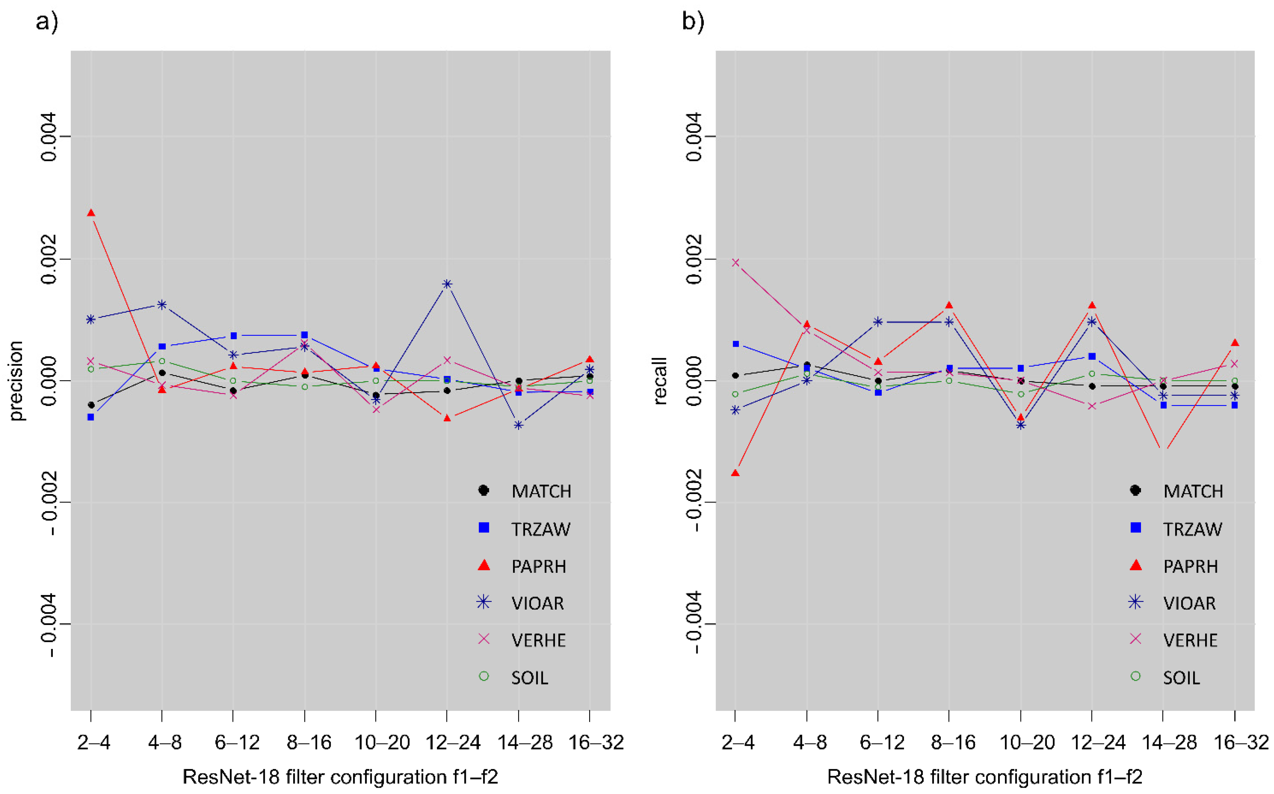
3.1. Overall Performance of the ResNet-18 Image-Level Classifier Regarding 32-Bit and 16-Bit Precision

The image-level classifier was tested using different filter configurations with the embedded system Jetson AGX Xavier. In general, an increasing trend for the overall accuracy with an increasing number of filters was determined (Table 2). The most gain in overall accuracy was found within the lower filter configuration from 2/4 to 6/12. In the higher filter configurations, overall accuracy was well above 90%, indicating strong predictive capabilities of the models. When changing the computation precision of the model from 32- to 16-bit, only a slight deviation was determined with values below 0.001. This was retrieved in the same way for the individual classes (Figure 6). No class had a higher deviation from the 32-bit models than 0.003 regarding precision and recall. Thus, the differences between 32- and 16-bit precision are negligibly small, and the use of 16-bit precision showed no detrimental effect on model quality in this study.
In Figure 7, the evaluation speed was recorded for one test image for the patch-level and the image-level classifier. The patch-level classifier uses no optimization in the prediction pipeline and works as if predicting on the image patch by patch independently, which is of course much more inefficient regarding computation costs. The patch-level classifier resulted in evaluation times ranging from 1077 to 2321 s from lower to higher filter configuration with 32-bit resolution. This evaluation speed would be far too long for application with UAV for online mapping. With the image-level classifier, the evaluation speed was substantially reduced and ranged from 0.42 to 1.07 s, from lower to higher filter configuration in 32-bit resolution. This was a reduction of evaluation time with a factor around 2100 to 2600. The evaluation speed of the image-level classifier was further reduced by using the 16‑bit rather than the 32-bit resolution version (Figure 7c). Globally, the evaluation speed increased with increasing filter configuration. Yet, the increase was greater for 32-bit than for 16-bit precision. With higher filter configurations, the test images were nearly twice as fast classified as with 16-bit precision. In numbers, an image needed 0.79 s to be fully classified on the embedded system in 32-bit with filter configuration 10/20, whereas only 0.46 s was needed when 16-bit precision was used, which refers to 1.3 or 2.2 frames per second, respectively. The latter speed would be suitable for online evaluation on the UAV for mapping weeds in the fields. Thus, the remaining sections will only discuss model testing in 16-bit mode, because higher precision improves computational performance without sacrificing accuracy.

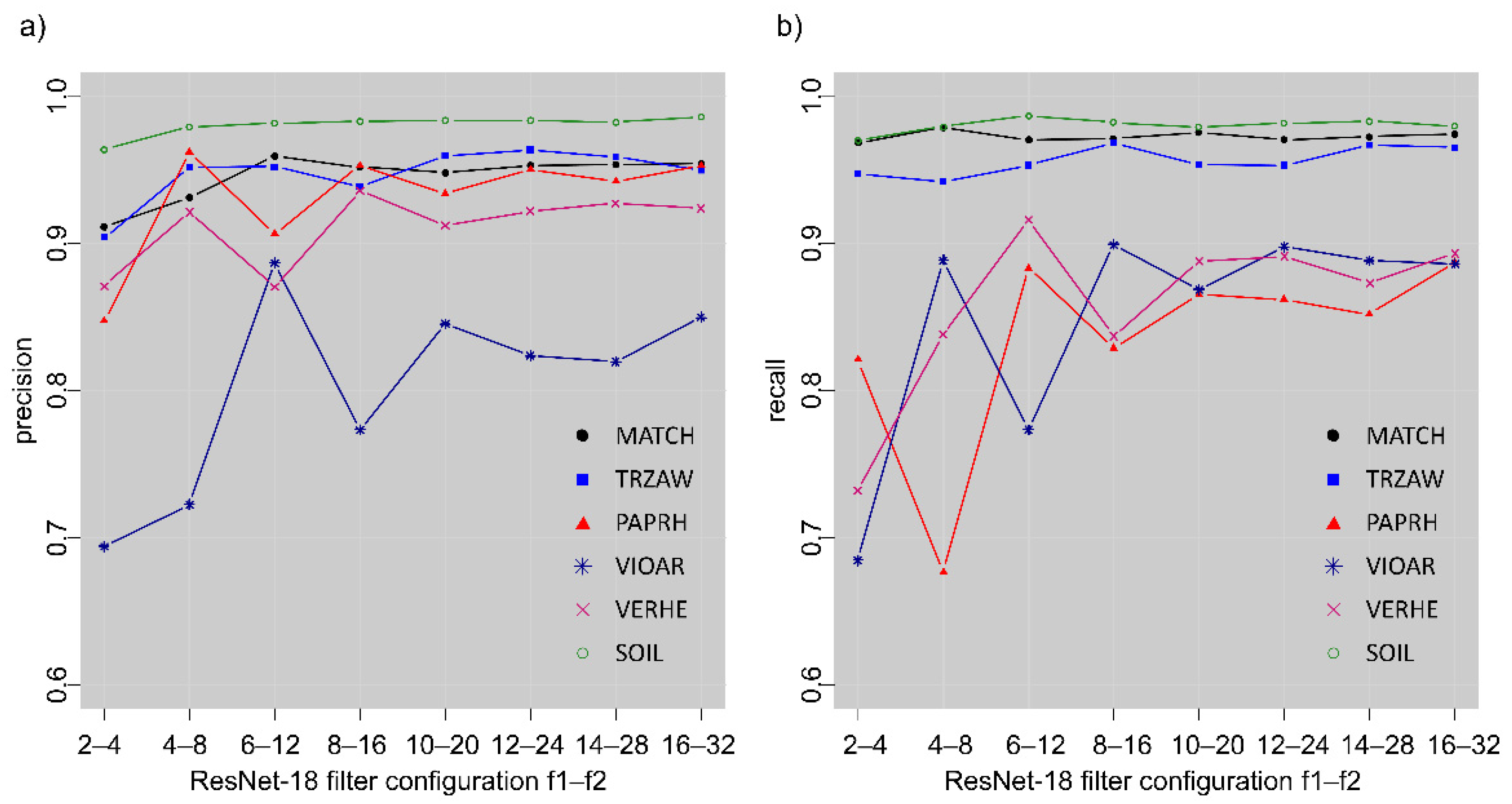
3.2. Class Specific Prediction Quality Assessment

In Figure 8, the precision and recall values are shown for the individual classes in relation to the filter configuration of the model. With a smaller number of filters integrated into the model, precision and recall are lower and indicate a more erratic characteristic from one filter configuration to the next. This effect is especially strong for the classes VIOAR, PAPRH, and VERHE and stronger for recall than for the precision statistic. With reaching filter configuration 10/20, precision and recall values stabilize for all models. The highest values for both precision and recall were received by the classes SOIL, TRZAW, and MATCH. For precision, the weeds PAPRH and VERHE reach also high values above 90%, but values for recall were below 90%. Obviously, the models tend to miss some of the PAPRH and VERHE plants, but those predicted to be PAPRH and VERHE are very likely to be actually present. Relatively, the worst model accuracy was obtained for the class VIOAR with values below 90% for precision and recall. However, with higher filter configurations greater than 10/20, VIOAR was still predicted with high quality with precision and recall values well above 80%.
In Table 3, a confusion matrix calculated from the models with filter configuration 10/20 is given calculated over all test images. The counts of five random seed outcomes were summarized with median. Overall, there was a strong differentiation of the models between plants and background as well as between crop and weed. The overall classification accuracy was 94%. Regarding the differentiation to the soil background, only for MATCH, a slight misclassification of the predictions was determinable. This misclassification might be related to the fact that leaves of MATCH are subdivided into many branches of small lobed leaflets. Therefore, the soil shines through the plant structure of MATCH, which might become hard to discriminate in some situations in the images for the models. Yet, misclassification rate was still on a very low level with a percentage below 1.2%. According to the confusion matrix, TRZAW was very well differentiated from the weed plants. There was only a weak confusion with MATCH, which might be attributed again to the transparency of the MATCH plants and to some extent to the remote similarity between them due to their ribbon-like plant structures.
Regarding the stability among the different seeds of the models, the models for SOIL, TRZAW, and MATCH had very little variation among them for precision and recall with coefficient of variation from 0.5% to 1.3% corroborating high consistency of model prediction. To some extent, this variation was higher for the weed species PAPRH, VERHE, and VIOAR, varying from 3.2% to 5.2%. Whereas MATCH, PAPRH, and VERHE or VIOAR were relatively well discriminated from each other, a more noticeable confusion occurred between VERHE and VIOAR with up to 10% of false predictions as VIOAR when it was in fact VERHE. Both weed species show a high degree of similarity, especially in the younger growth stages in which they were observed. In addition, both plants appeared very small with only very few remarkable features in the UAV images.
In Figure 9, a zoomed representation of an UAV aerial image is shown from the test set. This image was one of the images that were used to estimate a classification map with the image-level classifier on the embedded system. The classification map is shown on the left side of the figure for comparison. It appears that the incorporated class types are quite well-detected and outlined in the classification map. The background, SOIL class (in pink), covered not only the soil crust and aggregate structures, but also sporadically appearing stones in different shapes in the soil. The crop wheat, class TRZAW (in green), was found where it had grown densely and the leaves had a green appearance. Dead and unhealthy wheat leaves, however, were not detected by the image classifier. MATCH, which appeared quite frequently in the image (in red), was detected when it appeared in the open as well as when it densely appeared below the wheat crop. Thus, the image classifier showed abilities to differentiate the plants even when they overlapped each other. VIOAR (light blue) and VERHE (yellow) occurred less frequently and covered only small areas of the ground as individual plants, but were accurately detected by the image classifier when they appeared in the image. However, some limitations of the image classifier were also evident from the classification map of the test image shown in the figure. Although VERHE and VIOAR were precisely found in the test image, more areas of the image were assigned to VERHE and VIOAR than occurred in the field. These areas were mostly found between boundaries from one class to another, e.g., at edges of plant leaves. Probably an ambiguous structure appears in these areas of the image, which has a high similarity to another class. Another limitation can be seen in the bottom right part of the image. Here, a volunteer rapeseed plant appears. This plant species was not learned by the model and was also not learned from the background training images. Since information about the plant was not available in the model, the image classifier tries to assign the plant area to available class labels. It resulted in splitting this image area into TRZAW, VERHE, and PAPRH (dark blue) class labels.

4. Discussion

The optimized model approach for image-level classification presented in this study is fully convolutional and inherits the same features than the conventional ResNet-18 model for classification. The optimization could successfully increase evaluation speed for image classification of the UAV image, and it is implementable on an embedded system with online evaluation capabilities. Using the NVIDIA Jetson AGX Xavier board, a stable evaluation of 2.2 frames per second on the 3264 × 4912 px full-resolution images was reached in this study. Assuming a ground coverage of 2.25 m2 of the low altitude UAV imagery, this would result in an area performance of 1.78 ha h−1 for full, continuous crop field mapping. No loss of predictive capability was recorded when moving from 32-bit to 16-bit floating-point computation, but a huge gain in speed. It can be assumed that a further gain in speed will be achieved when shifting entirely to integer-based computation on the embedded board [45], which was not tested in this study. Area performance could also be increased with higher camera resolution to become more practical, as Peteinatos et al. [35] pointed out. However, another approach to enhance area performance could be sparse mapping. In this scenario, the UAV records images with gaps between the flight paths over the field, so that a faster mapping can be achieved. This can be combined with an overview UAV images taken from a higher altitude, which would give additional information for interpolating the weed map. Geostatistical interpolation methods, such as co-kriging or regression kriging, have been shown suitable to integrate UAV imagery information in the interpolation process as secondary information [46,47].
The image classifier was trained, optimized, and tested with the goal of later integration into an online weed detection system for winter wheat for UAV platforms. Thus, both the training and test images were not taken under controlled conditions where, for example, the camera was pointed directly at weed plants or the environmental conditions were controlled such that easy segmentation of individual weed, plant, or background features would have been possible. All images were captured from the copter platform with nadir perspective during low altitude flights. Some uncertainty is wanted in this study in order to assess the performance of the model under natural conditions. Thus, differences should be taken into account when comparing model performance with other studies. In general, the optimized image-classifier of this study performed with 94% overall classification accuracy, well in the range of studies aiming for classifying mixed weed plants [33,34,35,48,49]. In comparison with Pflanz et al. [11], a higher overall accuracy could be obtained on the same data set. The better performance was particularly striking for the similar weed species VIOAR and VERHE. This might indicate that deep residual networks are better suitable than bag of visual words approaches for the classification and discrimination of weed species in UAV imagery. In contrats to segmentation models, which would also produce a pixel-level segmentation into different classes of a given input image by being directly fully convolutional [41], our approach does not need segmentation-level labeling in the training data. This trades off to some extent model accuracy and annotation effort, because patch-labeling is not as accurate as segmentation-labeling, as it also includes labels, where wheat or weed plants did not exactly fit into the patch or labels or where background objects were also present next to the object of interest. Therefore, this noise may have also impacted model accuracy.
The UAV approach shown here does not need sophisticated camera technology. The network was trained from images captured by a snapshot RGB camera. Principally, this approach can be duplicated at rather low costs, especially if drone technology and computation technology drop further in prices. In perspective, drone swarms would allow mapping entire fields for weeds in minutes. Fast available weed maps achieved by UAV remote sensing might pave the way forward to accelerate the adaptation of SSWM technology. In previous experiments with an optoelectronic and camera-based weed sensor conducted in farmers’ fields of cereal and pea average, herbicide savings of up to 25.6% could be reached with SSWM [50]. They might also pave the way for selective weed management using fast-reacting direct injection sprayers [51,52]. Gerhards and Christensen [53] used tractor-carrying bispectral cameras for weed detection. In small row crops, winter wheat and winter barley, they reached herbicide savings with application maps depending on the level of weed infestation with even more than 90% by leaving such areas unsprayed where a certain treatment threshold was not reached. With the weed detection approach presented here, it should be possible in the future to identify and localize the key weeds that are important for wheat cultivation. This will contribute to adapted and more environmentally compatible crop protection and reduce the inputs of unwanted amounts of crop protection into the environment and the soil.

5. Conclusions

The approach presented in this study could successfully optimize a ResNet-18 DCNN classifier to differentiate crops, soils, and weeds as well as individual weed species from very high-resolution UAV imagery captured from low altitudes. Due to the optimization, the classification model can be efficiently applied to overlapping image patches in large images without leading to redundant computations in the convolution layers. This is achieved by computing the fully convolutional part of the model directly over the large, full-resolution UAV images instead of performing them patch-by-patch with a sliding window approach. The image-level classifier is guaranteed to give exactly the same predictions as independently applying ResNet-18 classification models to the image patches and therefore shares all its advantages for prediction. The performance with a ResNet filter configuration of 10 in the shallow and 20 in the deeper part of the network was found to be the best trade-off between accuracy and performance. Full-image evaluation under these settings was about 2.2 frames per second on an NVIDIA Jetson AGX Xavier board in 16-bit precision. It was found that when shifting from 16-bit to 32-bit precision, no improvement in accuracy was observed, but an increase in time cost of about a factor two for image evaluation. The performance enables implementation on a UAV platform for online mapping of weeds for crop fields. Assuming a constant speed and image processing of the UAV platform, this would amount to about 1.78 ha h−1 area output when mapping is performed continuously without any gaps from image to image. The image classifier achieved an overall accuracy of 94% when mapping the UAV aerial images of the test field. The classified images quite accurately distinguished weed species learned by the model, even in more complicated areas of the aerial imagery where plants overlapped each other. There are still limitations of the model regarding the classification of unknown species that need to be addressed to improve the transferability of the model to other crop fields.

Author Contributions

Conceptualization: T.d.C., M.S. and N.L.; methodology: T.d.C. and N.L.; programming: T.d.C. and N.L.; validation: M.P., M.S. and K.-H.D.; formal analysis: M.P.; investigation: M.S.; resources: N.L. and M.P.; data curation: M.P.; writing: M.S., N.L., T.d.C., M.P. and K.-H.D.; visualization: M.S., N.L. and T.d.C.; supervision: M.S. and M.P. All authors have read and agreed to the published version of the manuscript.

Funding

This research received no external funding.

Institutional Review Board Statement

Not applicable.

Informed Consent Statement

Not applicable.

Data Availability Statement

No new data were created or analyzed in this study. Data sharing is not applicable to this article. The code is available on GitHub repository: https://github.com/tiborboglar/FastWeedMapping.

Acknowledgments

We thank the staff of the JKI for their technical assistance, specifically Annika Behme and Werner Löhr for their precious assistance in annotating weeds and ground truthing in numerous field trials. We thank Dominik Feistkorn and Arno Littman for conducting the flight missions, and we thank Peter Zwerger for having made possible our investigations at his institute.

Conflicts of Interest

The authors declare no conflict of interest.

References

  1. Walter, A.; Finger, R.; Huber, R.; Buchmann, N. Opinion: Smart farming is key to developing sustainable agriculture. Proc. Natl. Acad. Sci. USA 2017, 114, 6148–6150. [Google Scholar] [CrossRef] [PubMed] [Green Version]
  2. Barroso, J.; Fernandez-Quintanilla, C.; Ruiz, D.; Hernaiz, P.; Rew, L. Spatial stability of Avena Sterilis Ssp. Ludoviciana populations under annual applications of low rates of imazamethabenz. Weed Res. 2004, 44, 178–186. [Google Scholar] [CrossRef]
  3. Zimdahl, R.L. Fundamentals of Weed Science, 3th ed.; Elsevier Academic Press: Amsterdam, The Netherlands, 2007; ISBN 978-0-12-372518-9. [Google Scholar]
  4. European Commission. EU Biodiversity Strategy for 2030 Bringing Nature Back into Our Lives; European Commission: Brussels, Belgium, 2020; Document 52020DC0380, COM(2020) 380 Final. [Google Scholar]
  5. Christensen, S.; Søgaard, H.T.; Kudsk, P.; Nørremark, M.; Lund, I.; Nadimi, E.S.; Jørgensen, R. Site-specific weed control technologies. Weed Res. 2009, 49, 233–241. [Google Scholar] [CrossRef]
  6. Jensen, P.K. Target precision and biological efficacy of two nozzles used for precision weed control. Precis. Agric. 2015, 16, 705–717. [Google Scholar] [CrossRef]
  7. Rasmussen, J.; Azim, S.; Nielsen, J.; Mikkelsen, B.F.; Hørfarter, R.; Christensen, S. A new method to estimate the spatial correlation between planned and actual patch spraying of herbicides. Precis. Agric. 2020, 21, 713–728. [Google Scholar] [CrossRef]
  8. Hunt, E.R.; Daughtry, C.S.T. What good are unmanned aircraft systems for agricultural remote sensing and precision agriculture? Int. J. Remote Sens. 2018, 39, 5345–5376. [Google Scholar] [CrossRef] [Green Version]
  9. Zhang, C.; Kovacs, J.M. The application of small unmanned aerial systems for precision agriculture: A review. Precis. Agric. 2012, 13, 693–712. [Google Scholar] [CrossRef]
  10. Schirrmann, M.; Giebel, A.; Gleiniger, F.; Pflanz, M.; Lentschke, J.; Dammer, K.-H. Monitoring agronomic parameters of winter wheat crops with low-cost UAV imagery. Remote Sens. 2016, 8, 706. [Google Scholar] [CrossRef] [Green Version]
  11. Pflanz, M.; Nordmeyer, H.; Schirrmann, M. Weed mapping with UAS imagery and a bag of visual words based image classifier. Remote Sens. 2018, 10, 1530. [Google Scholar] [CrossRef] [Green Version]
  12. Rasmussen, J.; Nielsen, J.; Garcia-Ruiz, F.; Christensen, S.; Streibig, J.C. Potential uses of small unmanned aircraft systems (UAS) in weed research. Weed Res. 2013, 1–7. [Google Scholar] [CrossRef]
  13. Paice, M.E.R.; Miller, P.C.H.; Bodle, D.J. An experimental sprayer for the spatially selective application of herbicides. J. Agric. Eng. Res. 1995, 60, 100–109. [Google Scholar] [CrossRef]
  14. Westwood, J.H.; Charudattan, R.; Duke, S.O.; Fennimore, S.A.; Marrone, P.; Slaughter, D.C.; Swanton, C.; Zollinger, R. Weed Management in 2050: Perspectives on the Future of Weed Science. Weed Sci. 2018, 66, 275–285. [Google Scholar] [CrossRef] [Green Version]
  15. Somerville, G.J.; Sønderskov, M.; Mathiassen, S.K.; Metcalfe, H. Spatial Modelling of Within-Field Weed Populations; a Review. Agronomy 2020, 10, 1044. [Google Scholar] [CrossRef]
  16. Walter, A.; Khanna, R.; Lottes, P.; Stachniss, C.; Nieto, J.; Liebisch, F. Flourish—A robotic approach for automation in crop management. In Proceedings of the 14th International Conference on Precision Agriculture (ICPA), Montreal, QC, Canada, 24–27 June 2018; pp. 1–9. [Google Scholar]
  17. Hunter, J.E.; Gannon, T.W.; Richardson, R.J.; Yelverton, F.H.; Leon, R.G. Integration of remote-weed mapping and an autonomous spraying unmanned aerial vehicle for site-specific weed management. Pest. Manag. Sci. 2020, 76, 1386–1392. [Google Scholar] [CrossRef] [Green Version]
  18. Yang, F.; Xue, X.; Cai, C.; Sun, Z.; Zhou, Q. Numerical simulation and analysis on spray drift movement of multirotor plant protection unmanned aerial vehicle. Energies 2018, 11, 2399. [Google Scholar] [CrossRef] [Green Version]
  19. López-Granados, F.; Peña-Barragán, J.M.; Jurado-Expósito, M.; Francisco-Fernández, M.; Cao, R.; Alonso-Betanzos, A.; Fontenla-Romero, O. Multispectral classification of grass weeds and wheat (Triticum Durum) using linear and nonparametric functional discriminant analysis and neural networks: Multispectral classification of grass weeds in wheat. Weed Res. 2008, 48, 28–37. [Google Scholar] [CrossRef]
  20. Peña, J.M.; Torres-Sánchez, J.; de Castro, A.I.; Kelly, M.; López-Granados, F. Weed mapping in early-season maize fields using object-based analysis of unmanned aerial vehicle (UAV) images. PLoS ONE 2013, 8, e77151. [Google Scholar] [CrossRef] [Green Version]
  21. De Castro, A.; Torres-Sánchez, J.; Peña, J.; Jiménez-Brenes, F.; Csillik, O.; López-Granados, F. An Automatic Random Forest-OBIA Algorithm for Early Weed Mapping between and within Crop Rows Using UAV Imagery. Remote Sens. 2018, 10, 285. [Google Scholar] [CrossRef] [Green Version]
  22. Choksuriwong, A.; Emile, B.; Laurent, H.; Rosenberger, C. Comparative study of global invariant descriptors for object recognition. J. Electron. Imaging 2008, 17, 1–10. [Google Scholar] [CrossRef]
  23. Franz, E.; Gebhardt, M.R.; Unklesbay, K.B. Shape Description of completely visible and partially occluded leaves for identifying plants in digital image. Trans. ASABE 1991, 34, 673–681. [Google Scholar] [CrossRef]
  24. Rumpf, T.; Römer, C.; Weis, M.; Sökefeld, M.; Gerhards, R.; Plümer, L. Sequential support vector machine classification for small-grain weed species discrimination with special regard to Cirsium Arvense and Galium Aparine. Comput. Electron. Agric. 2012, 80, 89–96. [Google Scholar] [CrossRef]
  25. Woebbecke, D.M.; Meyer, G.E.; Von Bargen, K.; Mortensen, D.A. Shape features for identifying young weeds using image analysis. Trans. ASAE 1995, 38, 271–281. [Google Scholar] [CrossRef]
  26. Csurka, G.; Dance, C.R.; Fan, L.; Willamowski, J.; Bray, C. Visual categorization with bags of keypoints. In Proceedings of the ECCV International Workshop on Statistical Learning in Computer Vision, Prague, Czech Republic, 15–16 May 2004; pp. 1–22. [Google Scholar]
  27. Kazmi, W.; Garcia-Ruiz, F.; Nielsen, J.; Rasmussen, J.; Andersen, H.J. Exploiting Affine Invariant Regions and Leaf Edge Shapes for Weed Detection. Comput. Electron. Agric. 2015, 118, 290–299. [Google Scholar] [CrossRef]
  28. Krizhevsky, A.; Sutskever, I.; Hinton, G.E. Imagenet classification with deep convolutional neural networks. In Proceedings of the Advances in Neural Information Processing Systems, Lake Tahoe, NV, USA, 3–6 December 2012; pp. 1097–1105. [Google Scholar]
  29. Lecun, Y.; Bottou, L.; Bengio, Y.; Haffner, P. Gradient-based learning applied to document recognition. Proc. IEEE 1998, 86, 2278–2324. [Google Scholar] [CrossRef] [Green Version]
  30. Szegedy, C.; Vanhoucke, V.; Ioffe, S.; Shlens, J.; Wojna, Z. Rethinking the Inception architecture for computer vision. In Proceedings of the 2016 IEEE Conference on Computer Vision and Pattern Recognition (CVPR), Las Vegas, NV, USA, 27–30 June 2016; pp. 2818–2826. [Google Scholar] [CrossRef] [Green Version]
  31. He, K.; Zhang, X.; Ren, S.; Sun, J. Deep residual learning for image recognition. In Proceedings of the 2016 IEEE Conference on Computer Vision and Pattern Recognition (CVPR), Las Vegas, NV, USA, 27–30 June 2016; pp. 770–778. [Google Scholar] [CrossRef] [Green Version]
  32. Russakovsky, O.; Deng, J.; Su, H.; Krause, J.; Satheesh, S.; Ma, S.; Huang, Z.; Karpathy, A.; Khosla, A.; Bernstein, M.; et al. ImageNet: Large scale visual recognition challenge. Int. J. Comput. Vis. 2015, 115, 211–252. [Google Scholar] [CrossRef] [Green Version]
  33. Dyrmann, M.; Karstoft, H.; Midtiby, H.S. Plant species classification using deep convolutional neural network. Biosyst. Eng. 2016, 151, 72–80. [Google Scholar] [CrossRef]
  34. Dos Santos Ferreira, A.; Matte Freitas, D.; da Silva, G.G.; Pistori, H.; Theophilo Folhes, M. Weed detection in soybean crops using ConvNets. Comput. Electron. Agric. 2017, 143, 314–324. [Google Scholar] [CrossRef]
  35. Peteinatos, G.G.; Reichel, P.; Karouta, J.; Andújar, D.; Gerhards, R. Weed Identification in Maize, Sunflower, and Potatoes with the Aid of Convolutional Neural Networks. Remote Sens. 2020, 12, 4185. [Google Scholar] [CrossRef]
  36. Simonyan, K.; Zisserman, A. Very deep convolutional networks for large-scale image recognition. arXiv 2014, arXiv:1409.1556. [Google Scholar]
  37. Zou, K.; Chen, X.; Zhang, F.; Zhou, H.; Zhang, C. A Field Weed Density Evaluation Method Based on UAV Imaging and Modified U-Net. Remote Sens. 2021, 13, 310. [Google Scholar] [CrossRef]
  38. Olsen, A.; Konovalov, D.A.; Philippa, B.; Ridd, P.; Wood, J.C.; Johns, J.; Banks, W.; Girgenti, B.; Kenny, O.; Whinney, J.; et al. DeepWeeds: A multiclass weed species image dataset for deep learning. Sci. Rep. 2019, 9, 2058. [Google Scholar] [CrossRef]
  39. Deng, J.; Zhong, Z.; Huang, H.; Lan, Y.; Han, Y.; Zhang, Y. Lightweight Semantic Segmentation Network for Real-Time Weed Mapping Using Unmanned Aerial Vehicles. Appl. Sci. 2020, 10, 7132. [Google Scholar] [CrossRef]
  40. He, K.; Zhang, X.; Ren, S.; Sun, J. Identity Mappings in Deep Residual Networks. In Computer Vision—ECCV 2016; Leibe, B., Matas, J., Sebe, N., Welling, M., Eds.; Springer International Publishing: Cham, Switzerland, 2016; Volume 9908, pp. 630–645. ISBN 978-3-319-46492-3. [Google Scholar]
  41. Long, J.; Shelhamer, E.; Darrell, T. Fully convolutional networks for semantic segmentation. arXiv 2015, arXiv:1411.4038. [Google Scholar]
  42. Kingma, D.P.; Ba, J. A Method for stochastic optimization. arXiv 2017, arXiv:1412.6980. [Google Scholar]
  43. Abadi, M.; Agarwal, A.; Barham, P.; Brevdo, E.; Chen, Z.; Citro, C.; Corrado, G.S.; Davis, A.; Dean, J.; Devin, M.; et al. TensorFlow: Large-scale machine learning on heterogeneous distributed systems. arXiv 2016, arXiv:1603.04467. [Google Scholar]
  44. Selvaraju, R.R.; Cogswell, M.; Das, A.; Vedantam, R.; Parikh, D.; Batra, D. Grad-CAM: Visual explanations from deep networks via gradient-based localization. Int. J. Comput. Vis. 2020, 128, 336–359. [Google Scholar] [CrossRef] [Green Version]
  45. Jacob, B.; Kligys, S.; Chen, B.; Zhu, M.; Tang, M.; Howard, A.; Adam, H.; Kalenichenko, D. Quantization and training of neural networks for efficient integer-arithmetic-only inference. In Proceedings of the IEEE/CVF Conference on Computer Vision and Pattern Recognition, Salt Lake City, UT, USA, 18–23 June 2018; pp. 2704–2713. [Google Scholar] [CrossRef] [Green Version]
  46. Jurado-Expósito, M.; de Castro, A.I.; Torres-Sánchez, J.; Jiménez-Brenes, F.M.; López-Granados, F. Papaver Rhoeas L. mapping with cokriging using UAV imagery. Precis. Agric. 2019, 20, 1045–1067. [Google Scholar] [CrossRef] [Green Version]
  47. Schirrmann, M.; Hamdorf, A.; Giebel, A.; Gleiniger, F.; Pflanz, M.; Dammer, K.-H. Regression Kriging for Improving Crop Height Models Fusing Ultra-Sonic Sensing with UAV Imagery. Remote Sens. 2017, 9, 665. [Google Scholar] [CrossRef] [Green Version]
  48. Lottes, P.; Behley, J.; Milioto, A.; Stachniss, C. Fully convolutional networks with sequential information for robust crop and weed detection in precision farming. IEEE Robot. Autom. Lett. 2018, 3, 2870–2877. [Google Scholar] [CrossRef] [Green Version]
  49. Sa, I.; Chen, Z.; Popovic, M.; Khanna, R.; Liebisch, F.; Nieto, J.; Siegwart, R. WeedNet: Dense semantic weed classification using multispectral images and MAV for smart farming. IEEE Robot. Autom. Lett. 2018, 3, 588–595. [Google Scholar] [CrossRef] [Green Version]
  50. Dammer, K.-H.; Wartenberg, G. Sensor-based weed detection and application of variable herbicide rates in real time. Crop Prot. 2007, 26, 270–277. [Google Scholar] [CrossRef]
  51. Rockwell, A.D.; Ayers, P.D. A variable rate, direct nozzle injection field sprayer. Appl. Eng. Agric. 1996, 12, 531–538. [Google Scholar] [CrossRef]
  52. Krebs, M.; Rautmann, D.; Nordmeyer, H.; Wegener, J.K. Entwicklung Eines Direkteinspeisungssystems Ohne Verzögerungszeiten Zur Pflanzenschutzmittelapplikation. Landtechnik 2015, 238–253. [Google Scholar] [CrossRef]
  53. Gerhards, R.; Christensen, S. Real-Time Weed Detection, Decision Making and Patch Spraying in Maize, Sugarbeet, Winter Wheat and Winter Barley: Patch Spraying. Weed Res. 2003, 43, 385–392. [Google Scholar] [CrossRef]
Figure 1. Proposed residual neural network architecture for classification of 201 × 201 px image patches. All convolution layers are followed by batch normalization layers and ReLU activations. Max pooling layers implement 2 × 2 maximum pooling with stride two. The final dense layer contains class scores for the six classes.
Remotesensing 13 01704 g001
Figure 2. Arrangement of the layers inside each of the residual blocks. Type A is shown on the left, and Type B is shown on the right. The number of filters for the conv layers varies from 16 to 32 depending on the residual block position.
Remotesensing 13 01704 g002
Figure 3. Architecture for image-level classifier derived from the patch-level model shown in Figure 1. Convolution and max pooling layers as well as residual blocks are identical to those in the patch-level model, except for their larger spatial dimension that results from the larger input size of the model. The cumulative local average pooling layer is a custom layer developed in this study and is described in Section 2.3. Together with the 1 × 1 convolution layer, it mimics the operation of the three last layers of the patch-level model (Figure 1) for each position in the grid.
Remotesensing 13 01704 g003
Figure 4. Model loss and accuracy on training the ResNet-18 model over 100 epochs.
Remotesensing 13 01704 g004
Figure 5. The heat maps of the ResNet-18 model show Grad-CAM images that highlight the importance of the area in the training image for model calibration.
Remotesensing 13 01704 g005
Figure 6. Differences between 32- and 16-bit resolution regarding model testing for precision (a) and recall (b) results in relation to filter configuration. Model results for each filter configuration were aggregated from five model runs with different randomization (seeds) of the weights.
Remotesensing 13 01704 g006
Figure 7. Evaluation speed for one UAV image in relation with filter configuration for the patch-level (a) and the image-level classifier (b) plus evaluation speed according to 16- or 32-bit resolution for the image-level classifier (16-bit—green line). In (c), the time difference between 16- and 32-bit resolution is shown for the image-level classifier. Model results for each filter configuration were aggregated from five model runs with different randomization (seeds) of the weights.
Remotesensing 13 01704 g007
Figure 8. Class specific precision (a) and recall (b) model performance on the test set in relation with filter configuration. Model results for each filter configuration were aggregated from five model runs with different randomization (seeds) of the weights.
Remotesensing 13 01704 g008
Figure 9. UAV aerial image with wheat crop and weed as zoomed in representation (left). In transparent colors (right): Superimposed classification resulting from the output of the ResNet-18 model with the optimized prediction routine running on an embedded system for the same UAV scene for comparison. The class labels are shown in different colors: SOIL (pink), TRZAW (green), MATCH (red), VERHE (yellow), VIOAR (light blue), and PAPRH (dark blue).
Remotesensing 13 01704 g009
Table 1. ResNet-18 model filter configuration and training parameters used for the patch-level and image-level classifier.
Filter 1Filter 2OptimizerLearning Rate
24Adam0.01
48Adam0.01
612Adam0.01
816Adam0.01
1020Adam0.01
1224Adam0.01
1428Adam0.01
1632Adam0.01
Table 2. Overall accuracy of prediction of the ResNet-18 model in 32-bit and 16-bit precision along with the difference between 32- and 16-bit shown in different filter configurations.
Filter 1Filter 232-Bit16-BitDifference
240.8830.883−0.000222
480.9160.916−0.000345
6120.9350.935−0.000098
8160.9300.931−0.000295
10200.9380.9380.000148
12240.9410.941−0.000172
14280.9390.9380.000197
16320.9440.9440.000000
Table 3. Confusion matrix for the evaluation on the test set for the image-level classifier using the ResNet-18 model with filter configuration 10(20). The resulting counts were agglomerated from five random seeds by median. CV refers to the coefficient of variation computed from the different outcomes of recall or precision expressed in percentage.
MATCHTRZAWSOILPAPRHVERHEVIOARRecallCV (%)
MATCH2307131758150.980.68
TRZAW21951241170.951.31
SOIL29117980170.980.67
PAPRH184356235230.874.40
VERHE81125739660.895.19
VIOAR47103148512930.895.01
Precision0.950.960.990.950.840.92Overall
CV (%)1.111.050.454.065.663.22accuracy0.94
Publisher’s Note: MDPI stays neutral with regard to jurisdictional claims in published maps and institutional affiliations.

