Self-Supervised Monocular Depth Learning in Low-Texture Areas

Abstract

For the task of monocular depth estimation, self-supervised learning supervises training by calculating the pixel difference between the target image and the warped reference image, obtaining results comparable to those with full supervision. However, the problematic pixels in low-texture regions are ignored, since most researchers think that no pixels violate the assumption of camera motion, taking stereo pairs as the input in self-supervised learning, which leads to the optimization problem in these regions. To tackle this problem, we perform photometric loss using the lowest-level feature maps instead and implement first- and second-order smoothing to the depth, ensuring consistent gradients ring optimization. Given the shortcomings of ResNet as the backbone, we propose a new depth estimation network architecture to improve edge location accuracy and obtain clear outline information even in smoothed low-texture boundaries. To acquire more stable and reliable quantitative evaluation results, we introce a virtual data set in the self-supervised task because these have dense depth maps corresponding to pixel by pixel. We achieve performance that exceeds that of the prior methods on both the Eigen Splits of the KITTI and VKITTI2 data sets taking stereo pairs as the input.

1. Introction

Depth estimation from a single image is a critical computer vision task in helping computers to understand real scenes. It is widely used in autonomous driving, augmented reality, and scene reconstruction. The recent advances in deep convolutional neural networks (CNNs) enable depth estimate using supervision from LiDAR measurements. However, ground-truth information from the expensive LiDAR [1] only provides sparse depth maps compared with image pixels. For transparent and dark surfaces, LiDAR also suffers greatly. As an alternative, self-supervised approaches leverage geometrical constraints on stereo images or image sequences as the sole source of supervision.

However, judging from the results running on standard benchmarks, there is still a gap between the self-supervised and the fully-supervised methods. Previous researchers assumed that no pixels violate the assumption of camera motion when using stereo pairs as the input for self-supervision. As such, the problematic pixels in low-texture areas have been ignored; moving objects and the occlusion problem have attracted more attention. As the main supervision function, photometric loss only computes the pixel difference between the warped source view and target view. In textureless regions, a target pixel usually corresponds to several candidate points in the source image, seriously affecting the accuracy of depth estimation. Recent works have partially mitigated the effects of this problem by adding smoothness loss [2,3] as extra supervision, but this method causes over-smooth boundaries. ResNet [4], as the backbone network, has some structural defects when applied to depth estimation since it was designed for classifying cases. For example, the receiving field of the network is too small to cope with less-textured areas and it cannot effectively preserve the spatial structure.

For pixels in areas with less texture, we solve them from two aspects: backbone network structure and loss function, while improving the estimation accuracy, to obtain clear object contour information. Because of the propagation of image gradients with a limited range, feature maps of the lowest level serve as images for photometric loss supervision, forming desirable loss for easier optimization. Additionally, first-order smoothness adding second-order smoothness together forms a smoothing function that forces the depth to propagate from the distinguished area to the less-textured areas.

Compared with preceding work that only prioritized engineering the loss function [2,5] in self-supervised depth estimation, we argue that performance hinges on the backbone networks, in line with the observations of [6]. Designing the backbone network to meet the depth estimation task requirements is still the key. ResNet [4], as the backbone network, has some defects when used for depth estimation tasks since it was designed for classified cases. Going beyond classification cases such as ResNet, our main contribution is a new convolutional network architecture for estimating depth using high-resolution images in a self-supervised manner. For the encoder, our architecture improves the structure of ResBlock and changes the number of channels to promote information flow propagation efficiency. For the decoder, the skip-connection is redesigned following the new encoder to better fuse features.

1.1. Overall Structure

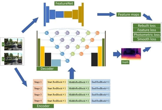
In general, our contributions can be summarized into three aspects: (1) A novel depth estimation backbone network is proposed to preserve the spatial structure and fuse semantic information more efficiently. (2) An improved loss function is redesigned to encourage the learned features propagation from discriminative regions to textureless regions. (3) A novel evaluation approach based on virtual data is first applied to self-supervised depth estimation. These combined improvements proce excellent results, outperforming prior methods using rectified stereo pairs. Figure 1 shows our overall architecture.

1.2. Related Work

Here, we concentrate on research related to depth estimation and the relevant review literature. Based on the different supervision methods, this task can be divided into supervised and self-supervised approaches.

1.2.1. Supervised Monocular Depth Estimation

Without a second input image for triangulation, acquiring absolute or even relative depth merely from a single image seems to be an ill-conditioned problem. Nevertheless, learning-based approaches show tremendous ability to fit predictive models taking images paired with depth maps as the input.

Eigen et al. [7] were the first to propose a two-scale deep neural network trained on an RGBD data set. The coarse network of the depth estimation architecture can predict global information, and then the fine network acquires local information. They changed the depth estimation architecture into a multi-task, which predicted depth, label, and normal simultaneously [8]. Laina et al. [9] abandoned the fully connected layer and adopted a convolution layer instead, leaving the entire network as an encoder–decoder process. Ramamonjisoa et al. [10] introced a refined net, predicting sharp and accurate occlusion boundaries using displacement fields. However, fully supervised approaches face challenges when acquiring ground-truth depth ring training. Thus, much work has exploited weakly supervised methods in the form of supervised appearance matching terms [11], parse ordinal depths [12,13], and known object sizes [14]. However, these methods cannot overcome the dilemma of collecting ground truth. Recent works focused on synthetic training data [15], but the dominant gap between the real image and synthetic data remains insurmountable. Given the difficulty of obtaining ground truth, supervised methods have reached a bottleneck, which has pressured researchers to explore self-supervised monocular depth estimation.

1.2.2. Self-Supervised Monocular Depth Estimation

Learning to predict depth without labels is a powerful concept e to the geometrical relationships between multiple captures of the same scene. The self-supervised approach training models use reconstructed images as the supervisory signal. Owing to this architecture taking monocular sequences or stereo pairs as the input, we review related works in two categories.

This method takes rectified stereo pairs as the input ring training and predicts the pixel disparities between the left and right images. Then, the trained model can estimate depth by inputting a single image for a test. Garg et al. [16] were the first to research self-supervised depth estimation using stereo pairs. A left–right depth consistency loss added as training loss in [17] proced results superior to the contemporary supervised methods. Various approaches, such as adopting semi-supervised data [18], leveraging generative adversarial networks [19], and using it in real-time [20], resulted in superior scores. Recently, semi-global matching (SGM), as additional supervision, was added for the monocular depth estimation task, which achieved excellent results [21]. Owing to rectified stereo pairs needing to be available in training, this method is not convenient for the depth estimation task.

A less constrained way, the self-supervision approach takes sequences as the input. Here, in addition to estimation depth using the geometric relationship between adjacent frames, this method also predicts the camera pose between frames.

Zhou et al. [22] published pioneering work predicting the camera pose between adjacent frames using PoseCNN. The architecture only relies on the geometric correlation between monocular video data for training. This work has been extended to multi-task learning [23], point-cloud alignment [24], and differentiable DVO [25]. To cope with moving objects that violate camera motion assumptions, Yin et al. [5] used optical flow to compensate for moving pixels, and Gordon et al. [26] leveraged segmentation masks to ignore the pixels that break the motion assumptions.

Others have focused on geometric priors. Depth–normal consistency loss [3] and 3D consistency loss [24] were proposed to improve the accuracy of depth estimation. Godard et al. [27] introced minimum re-projection loss and auto-masking, which became the most widely used baseline. Based on feature representation, feature-metric loss [28] was defined to solve low-texture pixels.

Some work has focused on the depth estimation backbone network. A generative adversarial network model [29] was proposed to address the monocular scenario. Guizilini et al. [30] exploited novel symmetrical packing and unpacking blocks to retain complete spatial information using 3D convolutions. Lyu et al. [31] improved the skip-connections of the decoder and added a feature fusion to quickly and efficiently process high-resolution images.

2. Materials and Methods

Here, we describe our backbone network for monocular depth estimation in detail. In Section 2.1, we mainly introced the proposed depth estimation backbone network. The entire network, as a U-net, is divided into two parts: encoder and decoder. Section 2.1.1 to Section 2.1.3 mainly introces the encoder, and Section 2.1.4 mainly introces how to decode. The architecture was designed to promote the flow of feature maps smoothly and reserve spatial structure as much as possible. To rece the semantic gap, we redesigned the skip-connection following our encoder by adding nodes between the encoder and decoder feature maps. In Section 2.2, we mainly introce the loss function based on feature representation and depth smoothness, effectively tackling low-texture areas, which is applied to supervise the optimization of the backbone network. The overall structure and interrelationship are shown in Figure 1 in Section 1.

2.1. The Backbone Network of Depth Estimation

Although the efficiency and effectiveness of monocular depth estimation in a self-supervised manner have been considerably improved, the backbone network still uses ResNet, which provides versatility and molarity. This architecture was designed for classification. When applied to the downstream field of depth estimation, there are still some structural defects, such as the receptive field of the network being too small to store space and semantic information. In order to deal with this situation and inspired by [32,33], we improved the ability of the encoder to obtain spatial information and promote the smooth flow of information.

2.1.1. Improved Information Flow through the Network

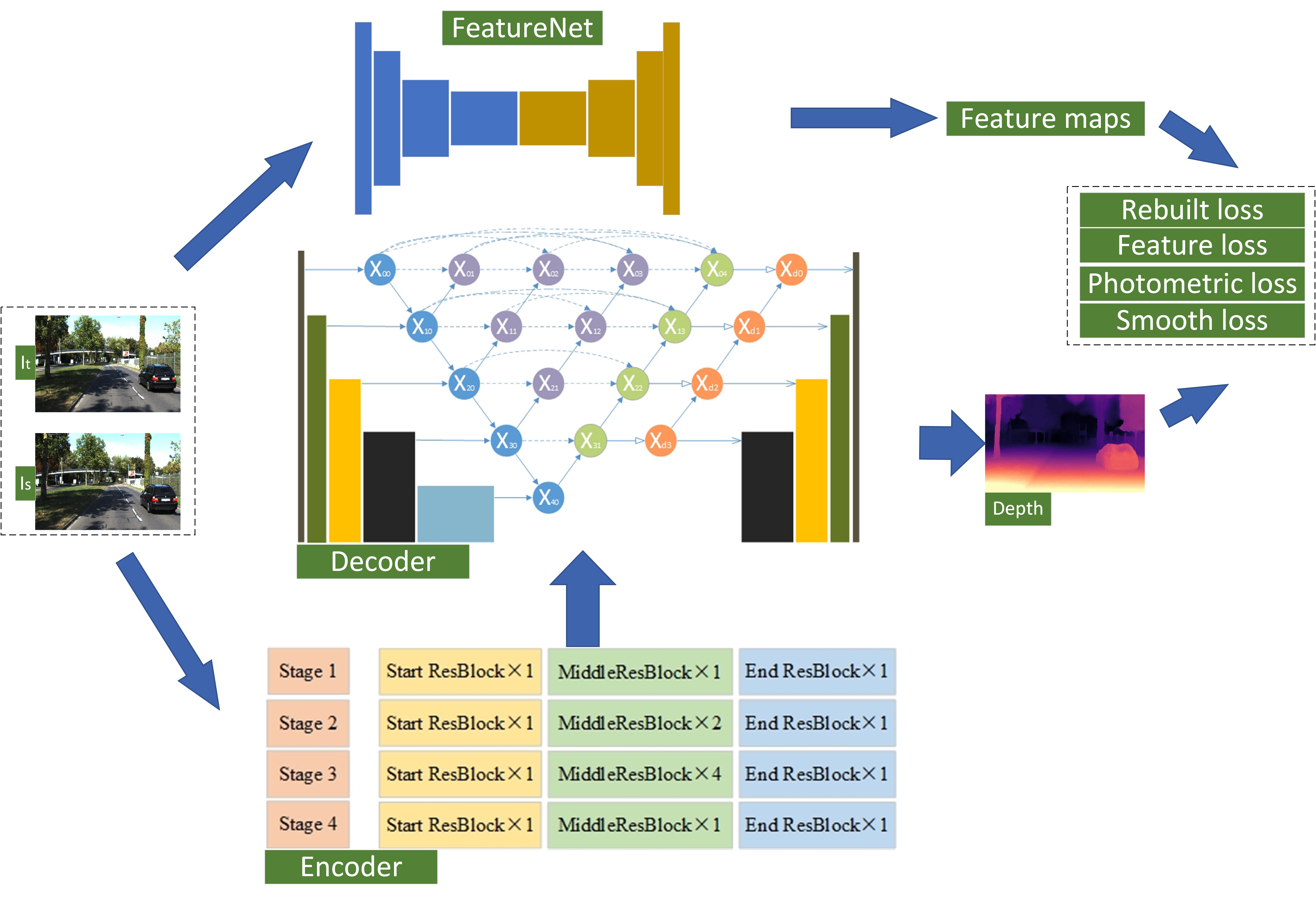
Depending on the number of network layers, ResNet is stacked by a corresponding number of building blocks (ResBlock), as shown in the left part of Figure 2. Each ResBlock can be defined as follows:

$$x^{l+1}=\left\{\begin{array}{c}ReLU(F(x^l,\left\{w_i^l\right\})+x^l);,\mathrm{if}\mathrm{size}\left(F(x^l,\left\{w_i^l\right\})\right)=\mathrm{size}\left(x^l\right);\hfill \\ ReLU(F(x^l,\left\{w_i^l\right\})+w_p^l{x}^l),\mathrm{if}\mathrm{size}\left(F(x^l,\left\{w_i^l\right\})\right)\ne \mathrm{size}\left(x^l\right);\hfill \end{array}\right.$$

(1)

where $x^l$ and $x^{l+1}$ are the input and output vectors of the lth ResBlock, respectively; $ReLU$ represents the activation function; $F(x^l,\left\{w_i^l\right\})$ is a learnable resial function; and $w_p^l$ is a learnable linear projection matrix that allows mapping the size of $x^l$ to the output size of F, which exists only in case of not corresponding dimensions for performing the element-wise addition between F and $x^l$.

The ResBlock of ResNet contains a convolutional layer with a 3 × 3 kernel and two convolutional layers with a 1 × 1 kernel. Each convolutional layer is followed by a batch normalization (BN) layer and a ReLU layer. However, as shown in Equation (1) and Figure 2, there is a ReLU at the end of each ResBlock. This nonlinear mechanism zeroes the negative signals. In the process of back-propagation, this operation may discard some available information, which will adversely affect the propagation. In order to overcome such shortcomings, ref. [33] eliminated the last ReLU in each ResBlock bottleneck. However, leaving the main path completely free, the architecture will be uncontrolled. Although this method solves the problem of information loss, it creates to two other dilemmas: in the overall four stages, there is no non-linearity mechanism in the main path, limiting the learning capability; with the continuous stacking of blocks and no BN layer after addition, non-standard signals will cause learning difficulties. To stabilize the information flow, inspired by [32], we ensured that each stage possesses only one nonlinear mechanism and one normalization (BN) at the end of the ResBlock.

To fairly compare our method with previous approaches, our backbone network uses 50 layers, although this ResBlock can be extended deeper. As shown in Figure 3, we have four downsampling stages as ResNet50, but different from ResNet50, which is consistent with every ResBlock, each stage in our structure contains three types: Start ResBlock, End ResBlock, and Middle ResBlock. The first stage includes a Start ResBlock, a Middle ResBlock, and an End ResBlock in turn. The second stage has a Start ResBlock, two Middle ResBlocks, and an End ResBlock linked in sequence. The third stage has a Start ResBlock, four Middle ResBlocks, and an End ResBlock. The fourth stage contains a Start ResBlock, a Middle ResBlock, and an End ResBlock in turn. For the Start ResBlock, there is a BN layer following the last Conv 1 × 1, which provides a normalized signal. For the End ResBlock, there is a BN layer and a ReLU on the main path after addition, which prepares and stabilizes the information flow into the next stage. In our case, only one ReLU stays on the main propagation path of each stage, retaining as many back-propagation weights as possible while maintaining the learning ability.

2.1.2. Improved Projection Shortcut

For aligning the spatial dimensions between x and the output of F, the projection shortcut mole is applied to ensure the element-wise addition. The mole contains a 1 × 1 Conv layer and a BN layer. In ResNet, when the stride of Conv is set to match the space size of output, it will skip 75% of the feature maps activation, losing a large mass of information. With no meaningful criterion, the remaining feature maps are considered by Conv 1 × 1. When the output of the projection shortcut is added to the main path, it contributes half of the information to the next ResBlock. This output of noise can negatively affect the main flow of information through the network.

In order to select more meaningful feature maps, considering as much information as possible, we use the max-pooling layer with a stride of 2 and select the element with the highest activation degree to the next step. As shown in Figure 4a, for ensuring element-wise addition computed over the same spatial window, we set the kernel of the max-pooling layer to 3, which is consistent with Conv to minimize content loss. Then, the selected feature maps perform Conv 1 × 1 with a stride of 1 to change the dimension for addition, which is followed by a BN layer. Another reason for having a max-pooling in the projection shortcut is to enhance the translation invariance of the network, and ultimately boost the learning performance.

2.1.3. Grouped Building Block

As we can see in the ResBlock of the original ResNet, the role of the two Conv 1 × 1 is to adjust the number of channels and align up and down, and Conv 3 × 3 is the only component able to learn spatial patterns. For practical considerations, Conv 3 × 3 runs on the least number of channels to control the computational cost and number of parameters.

To enhance the learning ability of the spatial structure, inspired by [32], we allocate Conv 3 × 3 as the maximum number of channels to obtain an improved learning ability. As shown in Figure 4b, we embrace grouped convolution to divide the input channels into several groups and perform the convolution operation independently for each group. This method can increase accuracy [34] while recing floating-point operations.

In summary, after three improvements, we only added a max-pooling layer to each projection shortcut. For a network with 50 layers, the increased number of parameters and calculations are negligible. On the contrary, with only four ReLUs on the backbone path, information flows through the network is smoother than in ResNet, so that it is faster than ResNet.

2.1.4. Skip Connections in the Decoder

Almost all depth estimation backbone networks adopt a U-Net structure, which increases the receptive field and restores the abstract features to the original size. As the core component of U-Net, skip-connection combines the deep semantic feature maps from the decoder subnet with the low-level feature maps from the encoder subnet. Based on long-skip, the traditional approach links the rich information of the input image and helps restore the information loss caused by downsampling. However, the feature maps from different layers are directly connected, which leads to fusion.

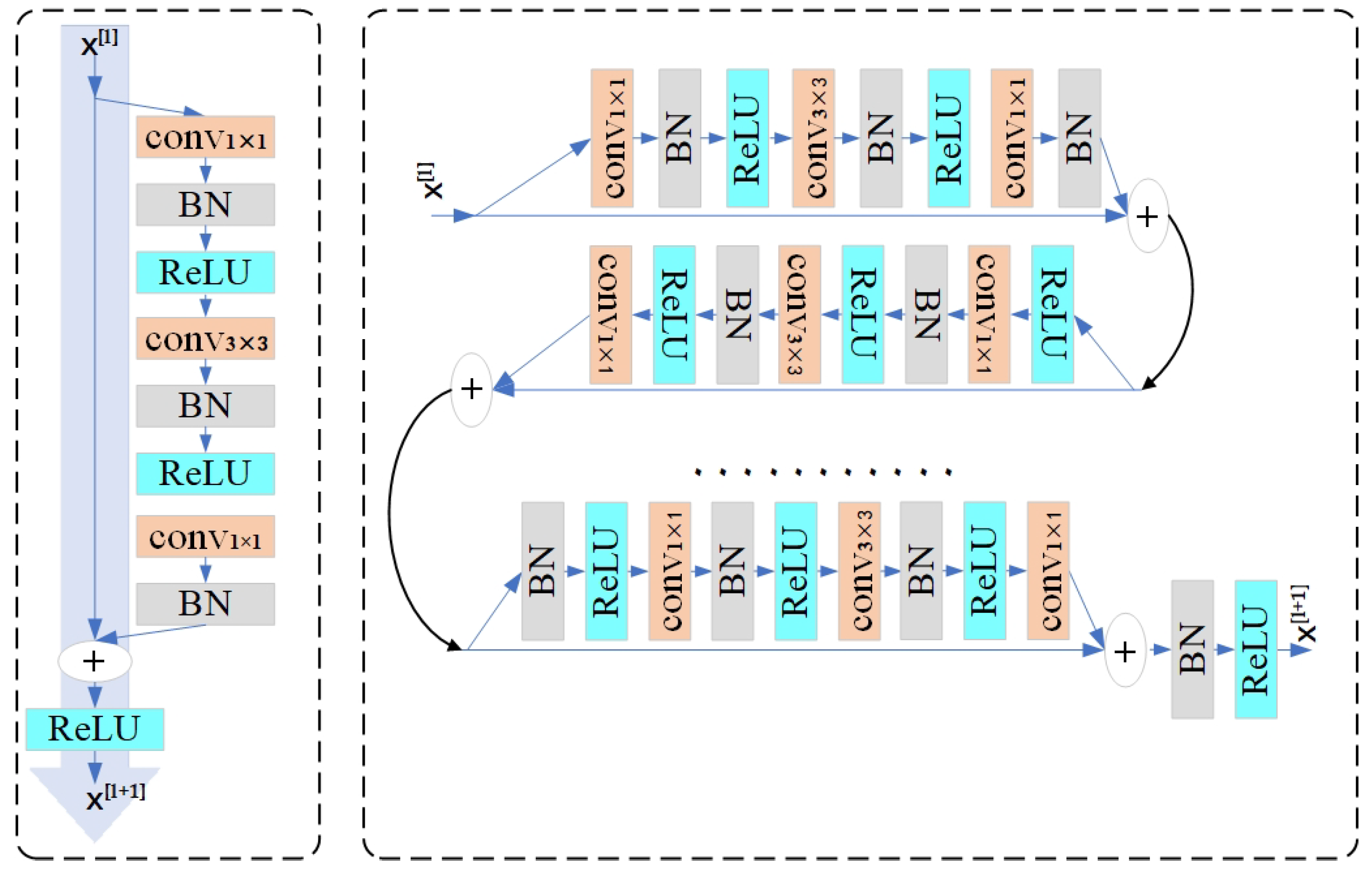
Inspired by [35], we redesigned the skip connection following our encoder to shorten the semantic distance between features at different levels. As shown in Figure 5, by adding nodes between the encoder and the decoder, the decoder maintains the advantages of short links while retaining long links. Each node integrates the upsampling information of all forward nodes of the same level and the corresponding node in the sublevel. The whole process of skip-connection is like a pyramid.

As indicated in a previous work [31], inaccurate depth estimation of an image in large-gradient regions is mainly e to semantically incorrect spatial information located on the boundary and classification errors. When feature maps of different levels have similar semantic features, the optimization process becomes easier and the fusion becomes effective. We can acquire depth maps more accurately by decoding these features. Let $x^{i,j}$ denote the output of node $X^{i,j}$ where i indexes the downsampling layer along with the encoder and j indexes the convolution layer of the dense block along the skip pathway. The stack of feature maps represented by $x^{i,j}$ is computed as

$$x^{i,j}=\left\{\begin{array}{cc}ReLU\left(U\left(x^{i-1,j}\right)\right)\hfill & j=0\hfill \\ ReLU\left([{\left[x^{i,k}\right]}_{k=0}^{j-i},U\left(x^{i+1,j-1}\right)]\right)\hfill & j>0\hfill \end{array}\right.$$

(2)

where $U(·)$ denotes an upsampling layer, and [ ] denotes the concatenation layer. Nodes only receive one input from the previous layer at level $j=0$; nodes acquire two inputs both from the encoder at two consecutive levels at level $j=1$; nodes at level $j>1$ acquire $j+1$ inputs, of which j inputs come from the outputs of the previous j nodes in the same level adding the last input, which is the upsampled output from the lower level. With the skip connection, all the preceding features are accumulated to the current node through the dense convolution block on each path. Therefore, each node receives multiple semantic level feature maps.

It is difficult to achieve ideal results only using convolution to aggregate information. Inspired by [31,35], we added a feature fusion squeeze-excitation block following each output node to boost fusion accuracy and efficiency. In the squeeze stage, the block aggregates feature maps by global average pooling to eliminate spatial interference. For the excitation operation, two fully-connected layers are followed by a sigmoid function to learn the importance of each feature. Finally, the scale value is learned through the network to reweight the feature map as the next level’s input. This mole builds the correlation between feature channels and enhances the mixing effect by enhancing valuable features.

2.2. Training Loss

2.2.1. Photometric Loss

The widely used supervision function, photometric loss, uses the structural similarity (SSIM) [36] term combined with the $L_1$ loss to estimate the pixel difference between a reconstructed view and the target view. The detailed form is given by emphasis Equation (3). In order to expand the data set, we did not apply the previous practice of only inputting the left images to reconstruct the right images, but randomly input the left and right images instead. Whether it is the left image or the right image, we collectively refer to the image input to the network as the target image $I_t$, and the image only used for the calculation of the loss function is called the source image $I_s$. The reconstructed target image is ${\widehat{I}}_t$. Therefore, the formula is:

$$L_p(I_t,{\widehat{I}}_t)=\alpha \frac{1-SSIM(I_t,{\widehat{I}}_t)}{2}+(1-\alpha )\parallel I_t-{\widehat{I}}_t\parallel$$

(3)

Benefitting from multi-view projection geometry, depth estimation in self-supervision methods has achieved remarkable results. However, when it comes to stereo pairs as the input, most of the previous works considered it unnecessary to deal with the pixel that violates the assumption of camera motion since this method only considers the relationship between the left and right frames. However, problematic pixels come from low-textured areas that are often ignored, which harm the photometric loss. Given the difficulty of tackling pixels in low-texture areas, we redefine the auto-mask [27] in our approach since it is designed for sequence cases. We also mask out the pixels that have a warped photometric loss $Lp(It,{\widehat{I}}_t)$ higher than their corresponding unwarped photometric loss $Lp(It,Is)$. This operation removes pixels that remain the same between the stereo pairs in low-texture areas.

$$M_p=L_p(I_t,I_s)>L_p(I_t,{\widehat{I}}_t)$$

(4)

The idea is that the mask should be zero when we want to ignore a pixel. Thus, the photometric loss is denoted as

$$L_{ph}=M_p\odot L_p$$

(5)

However, the auto-mask cannot completely resolve the problem from low-texture areas because of the weak supervision added as a photometric loss. The process of optimizing gradients with respect to depth depends on the image gradients. For low-texture regions, image gradients are close to zero, causing zero gradients for the optimization. Additionally, the inconsistent update directions toward the minimum can negatively affect the convergence of local non-smooth pixels.

The loss based on feature expression was proposed by [28], exploiting the lowest feature maps $\varphi \left(p\right)$ with gradient $\frac{\partial \left({\varphi }_s\left(\widehat{p}\right)\right)}{\partial \widehat{p}}$ to overcome the problem of optimization. However, this operation suffers from scale ambiguity because the loss is performed merely on the first scale. Owing to the depth maps and rotation matrices to warp source features being needed, we respect the design of photometric error and calculate feature loss on all scales, so that,

$$L_{\varphi }=\sum _p\sum _{i=1}^4\ell ({\varphi }_{si}\left(\widehat{p}\right),{\varphi }_t\left(p\right))$$

(6)

To be consistent with the photometric loss, we also add automask to feature loss, which can be rewritten as:

$$L_{\varphi m}=M_p\odot L_{\varphi }$$

(7)

Thus, the final photometric loss can be considered as follows:

$$L_{pf}=L_{ph}+L_{\varphi m}$$

(8)

To ensure that the correct features are available, we need a single-view reconstruction network as in [28] to learn the feature representation in a self-supervised manner. $L_{rec}$ is exploited to supervise the training for the network, which reconstructs its input for learning feature representation.

$$L_{rec}={\Sigma }_p\sqrt{{[I\left(p\right)-I_r\left(p\right)]}^2+ep{s}^2}$$

(9)

where $eps$ represents the non-negative minimum.

2.2.2. Disparity Smoothness Loss

To regularize the depth propagation from discriminative regions to textureless low-image gradient regions, a smoothness loss was added, which encourages first-order [17,27] or second-order smoothness [3]. However, such propagation is prone to over-smooth results around boundaries. Here, we add two regularizers $L_d$ and $L_c$, $L_d$ to explicitly encourage a large first-order gradient. $L_c$ is defined to penalize the second-order gradients by encouraging smoothness of feature and image gradients, ensuring consistent gradients in the course of optimization.

$$L_s=\sum _p|{\nabla }^1\varphi \left(p\right)|e^{-|{\nabla }^{1}I\left(p\right)|}+\sum _p|{\nabla }^2\varphi \left(p\right)|e^{-|{\nabla }^{2}I\left(p\right)|}$$

(10)

Thus, the training loss of our model is $L_{total}$, which can be written as:

$$L_{total}=L_{pf}+L_s+L_{rec}$$

(11)

2.3. Implementation Details

Our model for monocular depth estimation, implemented in PyTorch, is based on an encoder–decoder framework. It takes an image size of 320 × 1024 as the input and outputs multi-scale feature maps. Our model was run on four Tesla v100s, trained for 30 epochs using Adam, with a batch size of 6 for each graphics processing unit (GPU). We used the learning rate 0.0001 for the first 20 epochs, and then halved the learning rate for the remaining 10 epochs. The encoder of our 50-layer architecture adopts the improved ResBlock as mentioned, containing 23.37 million trainable parameters, which is less than the 25.56 million trainable parameters in ResNet-50. The speed of calculation is comparable to that of ResNet, while the effectiveness is significantly enhanced.

In order to obtain a stable feature representation of the image, we needed to rebuild a FeatureNet, which exploits an encoder consistent with DepthNet. The decoder contains five 3 × 3 convolutional layers and each is followed by an upsample layer. The network takes the original image as the input and acquires the reconstructed image. $L_{rec}$ is an extra regularizer to supervised training.

3. Results

Here, we describe the experimental proceres of monocular depth estimation using stereo pairs as the input in detail. The outstanding quantitative and qualitative performance of our approach is demonstrated. We also show the contribution of each component in the ablation study. In order to verify the generalization performance, we fed test data from the other data sets into our model and still obtained a reasonable estimate.

We assigned all images to the same intrinsic matrix. More specifically, the coordinates of the main point were from the geometric center point, and the focal length was the average value of each video sequence. For stereo pairs, the two cameras maintained a constant distance on the same horizontal line. Thus, we achieved the transformation between the two frames in one stereo pair through the baseline, without the need to estimate the pose between each other. We dropped median scaling for training with stereo pairs since the scaling is inferred from the known camera reference.

3.1. KITTI Eigen Split

We estimated the monocular depth on the KITTI 2015 data set [37] for a fair comparison with prior methods, which is the largest data set in autonomous driving including 200 street scenes captured by RGB cameras and a calibrated LiDAR device deployed near the left camera. Following the Eigen Split mentioned in [7], we divided the raw data set into two subsets: one included 697 frames from 29 scenes to serve as the testing set, and the other included 22,600 frames from 32 scenes to serve as training set. The ground truth was obtained from 3D points of the Velodyne laser reprojected onto 2D images.

We divided the experiment into two parts: the first using stereo supervision only, and the other adding an extra supervision method such as SGM or video. SGM is a traditional SGM-matching method used as a virtual label to supervise training, which effectively improves the performance in quantitative evaluation. According to

Table 1. Comparison of performance on the original KITII Eigen Split. The best results are in bold. S, trained on stereo pairs; MS, trained on calibrated binocular videos; †, trained using post processing steps. The metric in red is better. The metric in green is better.

Method	Train	Data Set	$\mathit{Absrel}$	$\mathit{SqRel}$	$\mathit{RMSE}$	${\mathit{RMSE}}_{\mathit{log}}$	$\mathit{\delta }<1.25$	$\mathit{\delta }<{1.25}^2$	$\mathit{\delta }<{1.25}^3$
Garg	S	K	0.152	1.226	5.849	0.246	0.784	0.921	0.967
StrAT	S	K	0.128	1.019	5.403	0.227	0.827	0.935	0.971
3Net(Rt50)	S	K	0.129	0.996	5.281	0.223	0.831	0.939	0.974
3Net(VGG)	S	K	0.119	1.201	5.888	0.208	0.844	0.941	0.978
MonoDepth	S	K	0.133	1.142	5.533	0.230	0.830	0.936	0.970
MonoResMatch	S	K	0.111	0.867	4.714	0.199	0.864	0.954	0.979
SuperDepth	S	K	0.112	0.875	4.958	0.207	0.852	0.947	0.977
MonoDepth2 †	S	K	0.105	0.822	4.692	0.199	0.876	0.954	0.977
RefineDistillHR	S	K	0.098	0.831	4.656	0.202	0.882	0.948	0.973
Ours	S	K	0.097	0.708	4.518	0.190	0.886	0.958	0.979
Ours †	S	K	0.097	0.700	4.507	0.190	0.886	0.958	0.979
EPC++	MS	K	0.128	0.935	5.011	0.209	0.831	0.945	0.979
MonoDepth2 †	MS	K	0.104	0.775	4.562	0.191	0.878	0.959	0.981
DepthHint	SGM + MS	K	0.098	0.702	4.398	0.183	0.887	0.963	0.983
Shu	MS	K	0.099	0.697	4.427	0.184	0.889	0.963	0.982
ours	MS	K	0.094	0.665	4.239	0.179	0.898	0.966	0.983
ours †	MS	K	0.093	0.650	4.202	0.178	0.899	0.966	0.983

, our method quantitatively outperformed the preceding self-supervised approaches on Eigen Split taking stereo pairs as the input.

The performance metrics for depth evaluation can be defined as follow:

$$AbsRel=\frac{1}{\left|D\right|}\frac{{\sum }_{dϵD}|d^{*}-d|}{d^{*}}$$

(12)

$$SqRel=\frac{1}{\left|D\right|}\frac{{\sum }_{dϵD}{∥d^{*}-d∥}^2}{d^{*}}$$

(13)

$$RMSE=\sqrt{\frac{1}{\left|D\right|}\sum _{dϵD}{∥d^{*}-d∥}^2}$$

(14)

$$RMSElog=\sqrt{\frac{1}{\left|D\right|}\sum _{dϵD}{∥log{d}^{*}-logd∥}^2}$$

(15)

$${\delta }_t:\frac{1}{\left|D\right|}\left|\left\{dϵD\right|max(\frac{d^{*}}{d},\frac{d}{d^{*}})<{1.25}^t\}\right|\times 100\%$$

(16)

where $d_{*}$ presents the ground-truth depth, d denotes the predicted depth, and $\left|D\right|$ is the number of predicted depth values.

Our proposed method obtained a significant drop in the squared error, which penalizes large errors in the short range more, as shown in Equation (13). Compared with the state-of-the-art approaches, the metric SqRel of our method decreases from 0.697 to 0.650. Since near objects are large in images, there are more low-texture pixels. Therefore, effectively recing such errors means that our method is more effective in processing low-texture pixels than the contemporary methods. Another closer result from the self-supervised methods was obtained by DepthHint, which has the same value in metric $\delta <{1.25}^3$.

Unlike the first four parameters that represent errors, $\delta <{1.25}^t$ denotes the percentage of the accuracy of the predicted value: the higher, better. DepthHint has the same ability as our method to control singular values. However, this approach uses the traditional stereo matching SGM method as an additional signal to supervise training. Although the performance is improved to a certain extent, it still uses photometric loss as the primary supervision method. Therefore, the architecture is likely to fall into local minima, which affects the optimization of the entire training process. On the contrary, our approach largely avoids the interference of local minima.

In addition to the quantitative comparison test, we concted a qualitative analysis, as shown in Figure 6. We provide the ground truth depth of the original image in the last column. Note that the KITTI dataset does not have point-by-point depth labels. We get ground truth depth based on the point clouds generated by Velodyne. As we all know, the point clouds of Velodyne serve as a benchmark for quantitative evaluation. However, the ground truth Velodyne depth being very sparse, we interpolate it for visualization purposes following previous works. Therefore, the image obtained in this way will have lots of holes and concentrated in the bottom of an image, which is an inherent problem of point clouds. The first two lines show that our approach can effectively tackle low-texture areas of nearby objects such as walls. It can also accurately locate the edge of the wall. As shown by the area in the green circle, our method not only deals with low-texture pixels but also obtains clear outlines when encountering billboards, road signs, and other objects, whereas these are submerged in pixels with grass as the background using monodepth2 in the third line. In the fourth line, our method can obtain homogeneous information and complete outlines of guideposts, but monodepth2 fails. Among the green circle in the fifth line, monodepth2 does not distinguish indivial characters, and the outlines are blurred when multiple people overlap. However, our method can portray a single character and even show the hand movements of a human. When encountering category overlap, we found that our model still provides excellent distinguishing performance. For example, in the green circle in the sixth row, the human body is distinguished from other categories, and there is no confusion like with the monodepth2 results. Finally, in a highly dynamic scene, our proposed method still effectively segmented the depth information of each instance.

Overall, we acquired preferable results in low-texture areas such as walls and guideposts, and detailed information is presented, such as the outlines of humans and poles. Since our model learns more accurate semantic information, it can distinguish different categories, even instances, in a scene.

3.2. Improved Ground Truth

The Eigen Split considers reprojected LiDAR points as ground truth for evaluation, which does not take moving objects and obstructions into account. To further verify the effectiveness of our method, we used the KITTI Depth Prediction Evaluation data set [27], which chooses 652 (or 93%) from the 697 test frames in the eigen test split. For addressing quality issues with the standard split, the improved ground-truth frameworks feature more accurate ground-truth depth. We evaluated the improved frameworks using the error metric consistent with the standard evaluation. The quantitative results of our method are still better than those of the previous approaches, as shown in

Table 2. Comparison of performance on the improved KITII Eigen Split. The best results are indicated in bold. S, trained on stereo pairs; MS, trained on calibrated binocular videos; †, using post processing steps. The metric in red is better. The metric in green is better.

Method	Train	Data Set	$\mathit{Absrel}$	$\mathit{SqRel}$	$\mathit{RMSE}$	${\mathit{RMSE}}_{\mathit{log}}$	$\mathit{\delta }<1.25$	$\mathit{\delta }<{1.25}^2$	$\mathit{\delta }<{1.25}^3$
Monodepth	S	K	0.109	0.811	4.568	0.166	0.877	0.967	0.988
3Net(R50)	S	K	0.102	0.675	4.293	0.159	0.881	0.969	0.991
SuperDepth	S	K	0.090	0.542	3.967	0.144	0.901	0.976	0.993
Monodepth2	S	K	0.085	0.537	3.868	0.139	0.912	0.979	0.993
ours	S	K	0.070	0.332	3.139	0.111	0.942	0.990	0.997
ours†	S	K	0.069	0.321	3.093	0.109	0.944	0.991	0.998
Monodepth2HR	MS	K	0.080	0.466	3.681	0.127	0.926	0.985	0.995
EPC++	MS	K	0.123	0.754	4.453	0.172	0.863	0.964	0.989
DepthHint †	SGM + MS	K	0.074	0.364	3.202	0.114	0.936	0.989	0.997
ours †	MS	K	0.070	0.298	2.931	0.104	0.945	0.993	0.998

.

3.3. Virtual KITTI

Neither the regular version nor the improved version of the data set is ideal for evaluation. The ground truth based on LiDAR has inherent flaws such as the points acquired being too sparse compared to image pixels and reliable reflections not being obtained on reflective or transparent surfaces. In order to obtain accurate pixel-by-pixel depth maps, we exploited the Virtual KITTI 2 data set [38], which is a synthetic data set fully annotated with realistic fidelity for the KITTI data set. We randomly selected 106 images from the clone setting to construct the test data set. Note that the error was only calculated in the lower half of the image since LiDAR scan points mostly appear in the lower half of the picture. Additionally, neither the baseline nor our approach received any training on VKITTI2 data. Although a domain gap between synthetic data and real data exists, we think this is the most effective estimation because the correspondence between labels and data is accurate and dense. As shown in

Table 3. Comparison of performance on the VKITTI2 data set. The best results are indicated in bold. MS, trained on stereo pairs; MS, trained on calibrated binocular videos; †, using post processing steps. The metric in red is better. The metric in green is better.

Method	Train	Data Set	$\mathit{Absrel}$	$\mathit{SqRel}$	$\mathit{RMSE}$	${\mathit{RMSE}}_{\mathit{log}}$	$\mathit{\delta }<1.25$	$\mathit{\delta }<{1.25}^2$	$\mathit{\delta }<{1.25}^3$
Monodepth2 †	MS	K	0.123	0.866	4.924	0.235	0.832	0.925	0.962
ours †	MS	K	0.108	0.700	4.822	0.204	0.839	0.943	0.980

, we still obtained excellent results.

3.4. Ablation Studies

To further explore the contribution of each part of our method to the overall performance, we concted an ablative analysis by changing the different architectural components that had been introced, as shown in

Table 4. The ablation study of different combinations. †, using post processing steps.

Method	$\mathit{Absrel}$	$\mathit{SqRel}$	$\mathit{RMSE}$	${\mathit{RMSE}}_{\mathit{log}}$	$\mathit{\delta }<1.25$
baseline †	0.105	0.822	4.692	0.199	0.876
encoder	0.101	0.753	4.509	0.192	0.885
encoder + feature-maps loss	0.100	0.724	4.511	0.192	0.885
Ours †	0.097	0.700	4.507	0.190	0.886

. The base architecture, Monodepth2, proced the worst effect, and all improvements combined performed the best.

The benefits of the encoder are that by adjusting the structure of ResBlock, the feature selection criteria are made meaningful, the spatial structure information is preserved, and the complete outline of the object is obtained.

According to the quantitative analysis in Table 4, dense skip connections effectively rece the semantic gap between feature maps at different levels e to long links. This architecture makes the fusion of feature maps between the encoder and decoder more efficient, the boundaries of different categories are more accurately located through clear semantic information, and then a complete outline of the object is obtained.

The benefit of feature loss are that the photometric difference is calculated using feature maps instead to cope with the neglected problem of pixels in low-texture regions. This approach ensures the learned features have gradients by explicitly encouraging a large gradient. As shown in Table 4, our method provides significant improvements in this task.

3.5. Additional Data Sets

In order to show the generalization performance of our depth estimation model, the Cityscapes [39] and Make3D [40] data sets were selected for testing. Note that we never used these data ring model training. Although there are differences between these data sets such as size, scene contents, and camera parameters, we were still able to draw reasonable inferences.

CityScapes uses stereo video sequences to record 50 different city street scenes, including 22,973 stereo pairs with a size of 2048 × 1024 pixels. However, the disadvantage is that there is a strongly reflective Mercedes-Benz logo at the bottom of the image, which will harm the results of inference. Therefore, only 80% of the original image was retained for testing. As shown in Figure 7, our method still achieved reasonable results on low-texture areas and on finer details such as cars, poles, and billboards, even if this type of data never appeared in the training process. In the first picture, the sign is in the pixels with the tree as the background, and our method still obtained the accurate outline information of the object. Although our method can better deal with low-texture pixels at close range, it does not perform well when encountering transparent surfaces such as the glass of cars in the third image. We treated it as a low-texture area, which only partially solved the problem.

Make3D has pixel-by-pixel labels, so the amount of data is small since it serves for fully-supervised tasks. Owing to the length–width ratio being different from KITTI data, we needed to cut it randomly in accordance with KITTI before feeding the network. The qualitative results are shown in Figure 8. This data set is different from the previous ones, being beyond the scope of the street landscape, and the platform for the data set collection is not a moving car, but a random shot, which poses considerable challenges to our inference process. However, judging from the test results, our model still obtained accurate results regarding the distances of various objects in the image such as people, poles, and trees.

4. Discussion

In this paper, improvements are made in three aspects: backbone network, loss function, and data set. Through a series of experiments including a qualitative evaluation, quantitative evaluation, and ablation research, we found that the reasonable backbone network architecture can proce more effective feature maps and improve the overall performance. An accurate loss function can make the entire optimization process more targeted for a specific application, such as processing pixels in low-textured areas. Other minor aspects such as resolution and post-processing can also improve the performance of quantitative evaluation, but the contributions are limited.

For quantitative experiments, we obtained impressive results that outperformed preceding methods by a large margin on the original Eigen test split, improved Eigen test split, or VKITTI test split. The parameter SqRel, which penalizes large errors in the short-range more, decreased by about 7% on the original Eigen test split, dropped below 0.3 for the first time and reaching 0.298 on the improved Eigen test split. These results showed the effectiveness of our model in dealing with pixels in low-texture areas. However, it is hard to upgrade the last parameter, which is the probability of singular values within a certain range. Whether it is evaluated on the original or improved Eigen test split, there are always methods that proce the same results as our method, meaning our approach is unable to surpass the contemporary methods on all evaluation parameters. We think that this is an inherent problem with stereo input. When inputting stereo pairs for training, only the relationship between the left and right pictures are considered. When using sequences instead, the relationship between multiple frames can be considered. In following research, we will focus on solving the above problems, improving the effect of self-supervised depth estimation, and close the gap between it and full supervision.

For quantitative evaluation experiments, we acquired better results on low-texture areas and finer details on objects such as cars, poles, and billboards, even these data were never used in the training process. Since our model learns more accurate semantic information, it can distinguish different categories, even instances, in the scene. However, our model still does not perform well when encountering transparent surfaces such as glass. This is an inherent problem in scene understanding. Data generated by sensors such as cameras and LiDARs will encounter such problem. We treated it as a low-texture area, which only partially solved the problem. We will focus on this problem in subsequent research.

5. Conclusions

In this work, we mainly focused on low-texture areas that are often overlooked, based on stereo pair input. We used feature maps instead of images to perform photometric loss supervision. Furthermore, the backbone network of depth estimation was redesigned, which boosts the flow of information in the network and improves the efficiency of aggregation between different levels. While preserving the complete spatial structure, the accuracy of location on edge is improved. Finally, we introced the VKITI2 data set with point-by-point depth labels for evaluation, and still achieved excellent results.