Article

Hyperspectral Image Classification across Different Datasets: A Generalization to Unseen Categories

1
Electronic Information School, Wuhan University, Wuhan 430072, China
2
Institute of Aerospace Science and Technology, Wuhan University, Wuhan 430072, China
*
Author to whom correspondence should be addressed.
Remote Sens. 2021, 13(9), 1672; https://doi.org/10.3390/rs13091672
Submission received: 1 April 2021 / Revised: 22 April 2021 / Accepted: 23 April 2021 / Published: 26 April 2021

Abstract

:
With the rapid developments of hyperspectral imaging, the cost of collecting hyperspectral data has been lower, while the demand for reliable and detailed hyperspectral annotations has been much more substantial. However, limited by the difficulties of labelling annotations, most existing hyperspectral image (HSI) classification methods are trained and evaluated on a single hyperspectral data cube. It brings two significant challenges. On the one hand, many algorithms have reached a nearly perfect classification accuracy, but their trained models are hard to generalize to other datasets. On the other hand, since different hyperspectral datasets are usually not collected in the same scene, different datasets will contain different classes. To address these issues, in this paper, we propose a new paradigm for HSI classification, which is training and evaluating separately across different hyperspectral datasets. It is of great help to labelling hyperspectral data. However, it has rarely been studied in the hyperspectral community. In this work, we utilize a three-phase scheme, including feature embedding, feature mapping, and label reasoning. More specifically, we select a pair of datasets acquired by the same hyperspectral sensor, and the classifier learns from one dataset and then evaluated it on the other. Inspired by the latest advances in zero-shot learning, we introduce label semantic representation to establish associations between seen categories in the training set and unseen categories in the testing set. Extensive experiments on two pairs of datasets with different comparative methods have shown the effectiveness and potential of zero-shot learning in HSI classification.

1. Introduction

Hyperspectral image (HSI) is characterized by a higher spectral resolution than conventional remote sensing images. It usually presents as a 3D data cube. HSI classification is one of the essential techniques in hyperspectral data analysis. It refers to classifying each pixel in the image based on spectral and spatial features. The rich spatial and spectral information in an HSI positively enhances the interpretation capability of remote sensing images, making HSI classification techniques attract widespread attention and widely used in environmental monitoring, precision agriculture, resource exploration, military reconnaissance, disaster assessment and other fields [1,2,3,4,5,6].
In recent years, the rapid development of hyperspectral imaging has remarkably reduced the cost of collecting hyperspectral data, especially since the successful implementation of miniaturization has improved the portability of hyperspectral sensors. It has stimulated a massive increase in HSI datasets, and various hyperspectral applications have given rise to strong demand for reliable and detailed annotations. It poses two significant challenges for HSI classification. Firstly, in the hyperspectral community, a vast amount of works for HSI classification has been developed recently, focusing on leveraging the richness of features [7,8]. Many of them have reached near-perfect classification performance on public hyperspectral datasets. However, it is worth noting that, unlike visual classification datasets, the HSI dataset is an individual data cube formed from hundreds of band images acquired by a hyperspectral sensor in the same scene [9,10]. Since labelling the hyperspectral data is quite laborious and expensive, the current hyperspectral domain has no such scale database like ImageNet [11]. Hence, almost all existing HSI classification methods are trained and evaluated in a single data cube [12,13]. Worse still, most of them take the random sampling strategy to split training and testing sets, which distributions of training and testing sets are shown in Figure 1b,c. Various semantic segmentation and HSI classification algorithms have demonstrated the importance of spatial features for model performance improvement [14,15,16,17]. When it comes to calculating spatial features in the neighbouring region, it easily results in an overlapping problem between the training set and the testing set in the spatial domain. It would make a possible over-optimistic estimation of classification performance [18,19,20]. Besides, only a tiny fraction of pixels in the existing public HSI dataset are labelled, while traditional supervised classifiers require sufficient labelled training samples for each category. It leads to an insufficient training sample problem. All these problems pose a threat to the further development of supervised learning-based classification methods. Second, as shown in Figure 1, different colour represents a different type of land-covers, and the spatial distributions of them described a kind of inherent characteristic of this scene. Datasets collected in other scenes usually have some degree of distinction in both spatial distributions and types of land covers, such as Indian Pines dataset [21], Salinas dataset [22], etc. It leads to poor performance when the trained models are directly generalized to new datasets [23,24,25]. Therefore, we need to develop a classification model that can be adapted to new datasets, including adapting the differences in spatial distribution and the new categories. This also places a high demand on the generalization ability of the classification models.
In this paper, we introduce a new paradigm for HSI classification to address the above limitations, where classification models are trained and evaluated across different datasets. It has hardly been studied in the hyperspectral community yet. Specifically, the classifier is trained on one dataset and evaluated on the other dataset. As mentioned earlier, evaluating another dataset would bring some new and unseen categories, so the main challenge under the new classification paradigm is to establish correlations between seen and unseen categories. The labels of hyperspectral categories are artificially defined based on the common knowledge of natural science. The semantic representations of such labels can be considered as a kind of high-level feature. Inspired by recent advances in zero-shot learning, we tackle the gap between seen and unseen categories by introducing word semantic representations. It provides the possibility to implement label prediction between different HSI datasets. We can obtain semantic representations of all labels and then establish associations between the learned categories in the training set and the unseen categories in the testing set in the same embedding space. Thus, for the task of training and evaluating classification models across datasets, our complete scheme can be divided into three phases, including feature embedding, feature mapping and label reasoning.
The main contributions of this work are as follows:
  • We break through the traditional paradigm of dividing training and testing data on a single data cube in the HSI classification. This work introduces a new paradigm for HSI classification that trains a classifier on one HSI dataset and tests on another. Specifically, a pair of HSI datasets captured from the same imaging sensor is selected to form the training set and the testing set, respectively.
  • The main challenge of HSI classification across different datasets is that the gap between those two datasets. Except for the difference in spatial distribution, there may be new and unseen categories in the testing set. The proposed solution is that employ word semantic representation of labels to narrow the gap between seen categories in the training set and unseen categories in the testing set. To the best of our knowledge, this is the first work to introducing semantic representations for HSI classification across different datasets.
The rest of this paper is organized as follows. Section 2 describes some related work, including zero-shot learning and word semantic representation. In Section 3, we present the problem setup. Section 4 introduces the details of the proposed three-phase scheme for HSI classification. Experimental results and implementation details are provided in Section 5. Section 6 concludes this paper and hints at plausible future research lines.

2. Related Work

This section describes the background and existing works that are most related to our research, including the development of zero-shot learning and label semantic representation.

2.1. Zero-Shot Learning

Zero-shot learning is aroused by humans’ ability to recognize new categories purely based on the learned high-level description. This kind of study aims to intelligently apply previously learned knowledge to help future recognition tasks, which has received increasing interest [26,27,28,29]. Contrary to this classic paradigm of supervised learning, zero-shot learning is to reason the label of the unseen category with learned knowledge, and the “zero” means no training examples [30,31,32].
As shown in Figure 2, the solution for zero-shot learning is to firstly employ side information, i.e., label semantic embeddings from external knowledge sources, to narrow the gap between the seen and unseen categories. Label semantic representations such as attributes and word vectors are common choices in zero-shot learning, both of them are high-level descriptions of the label [30,33,34]. The association between seen and unseen categories is established in the label semantic feature space. Then, the correspondence between semantic features and visual features is learned through feature mapping. Hence, such a correspondence can be transferred from seen categories to unseen categories.
Recent approaches have made significant success in zero-shot learning. Changpinyo et al. [26] assume that the cluster center of visual features are target semantic representations and leverage structural relations on the clusters to further regularize the model, and finally force the semantic representations to be predictive of their visual exemplars. Annadani et al. [28] devise objective functions that help preserve the structure of the semantic space in the embedding space by utilizing semantic relations between categories. Wang et al. [35] uses the latent-space distributions as a prior for a supervised variational autoencoder and presents a deep generative model for zero-shot learning.

2.2. Word Semantic Representation

As a tool for expressing ideas that have evolved over millions of years, words are not something that computers can understand. It has highly abstract characteristics. Word embedding is a kind of semantic representation, which can make natural language computer-readable [36,37]. By embedding words into a dense space, we can represent words numerically in a way that captures them in vectors that have tens or hundreds of dimensions instead of millions. It is one of the most vital techniques in natural language processing (NLP) [38].
Generally, the goal of constructing a word embedding space is to capture some sort of relationship in that space, be it semantic, morphology, context, or some other kind of relationship. Figure 3a shows the label semantic distributions of the Pavia Center dataset. Typically, words with similar meanings will have vector representations that are close together in the embedding space. Figure 3b presents the distance between different labels by the PCA two-dimensional projection.
Word2vec is a method to create word embeddings efficiently and has been around since 2013 [39]. Some of its concepts are effective in creating recommendation engines and making sense of sequential data even in commercial, non-language tasks [40]. Even better, some pieces of literature have proved that the pre-trained word embeddings can apply to many tasks [41,42]. The beauty is that different word embeddings are created either in different ways or using different text corpora to map this distributional relationship. Hence, word embeddings can help us with different down-stream tasks in many fields besides NLP.

3. Problem Definition

The main challenge of HSI classification across different datasets is to classify new categories that are unseen in the training process. Let Z TR = { z t r 1 , . . . , z t r s } denotes a set of s seen categories and Z TE = { z t e 1 , . . . , z t e u } symbolizes a set of u unseen categories. It should be emphasized that the testing set contains new categories, even without any intersection with the training set.
In this task, the training set is defined as TR = { ( x i t r , y i t r ) } i = 1 N t r , where x i t r X TR represents a labeled sample in the training categories and y i t r Y TR is its corresponding label, and a testing set is defined as TE = { ( x i t e , y i t e ) } i = 1 N t e , where x i t e X TE is a labeled sample in the testing categories and y i t e Y TE is the label of it. The goal of this task is to classify unseen testing samples by the knowledge learned from the training set.
First, to narrow the gap between the seen and unseen categories, a hyperspectral feature embedding function ϕ ( · ) is employed to extract the hyperspectral features of samples and project them into the common visual feature space,
ϕ : X X ˜ ,
where X ˜ R V is a hyperspectral embedding in V-dimensional visual feature space.
Since the training set and the testing set have no intersection, we have to utilize some auxiliary information to build the relationship between them. A typical assumption is that each category in Z TR and Z TE is associate with semantic embedding vectors in a common semantic feature space. We employ a label transformation model ψ ( · ) ,
ψ : Z Z ˜ ,
where Z ˜ R S is a semantic embedding in S-dimensional label semantic feature space. Through projecting the category of training and testing set into a joint label semantic embedding space, the inner-class connection between them is established.
Then, we construct hyperspectral feature ϕ ( x t r ) paired with label semantic feature ψ ( z t r ) on the training set through their label y t r to learn the mapping between them. Finally, the learned mapping is applied to the testing data to get the corresponding embedding, and the final label is derived by similarity measurement.
The final classifier f can be formed as:
f = g ( h ( ϕ ( x ) , ψ ( z ) ) ) ,
where h ( · ) indicates a mapping model between ϕ ( x ) and ψ ( z ) , usually learned from the training set, and g ( · ) can be a classification model based on a similarity metric.
Given the instance x i t e from TE , our aim is to estimate the label y i t e by a three-phase approach.
(A)
Employ ϕ ( · ) to embed x i t e into visual feature space, and ψ ( · ) to embed y i t e into label semantic feature space, respectively.
(B)
Learn a feature mapping h ( · ) between hyperspectral feature and label semantic feature on the training set.
(C)
Predict the embedding of testing data by the learned mapping h ( · ) , and infer its final label by a similarity metric g ( · ) .

4. Methodology

In this section, we give a detailed introduction of our method. We first introduce the overview of the framework, and then give the detailed information of the whole scheme in three phases.

4.1. Overview of the Framework

As illustrated in Figure 4, the whole scheme for HSI classification across different datasets can be described in three phases. Phase A is the feature embedding phase (see Figure 5), which aims to obtain the discriminative features ϕ ( x ) of HSI data as well as the semantic representation of the category labels ψ ( z ) to establish the association of the same kind of features in different datasets. Phase B is feature mapping (see Figure 6), in which we learn the correspondence h ( · ) between hyperspectral features and label semantic representations by feature mapping in the training set. Finally, in phase C, named the label reasoning phase (see Figure 7), we apply the learned mapping to the testing set and employ the similarity metric g ( · ) to reason about the final labels.

4.2. Phase A: Feature Embedding

4.2.1. Hyperspectral Feature Embedding

The origin HSI data are embedded into the hyperpsectral feature space by an HSI classification model. In general, the hyperspectral features are the middle-level output of a classification model. Various models have been proposed in the field of HSI classification [43,44,45,46,47]. The choice of model is flexible here, and three possible architectures are considered in our work.
The first choice is the recurrent neural network (RNN), which has advantages in sequence modeling. Mou et al. [48] firstly introduced RNN in HSI classification, which has proven that RNN can be used to extract abundant spectral features in HSI. Later, aiming at the contextual information among adjacent spectral, the bands-grouping strategy has been proposed by [49,50]. In this work, we adopt the bands-grouping RNN as the hyperspectral feature embedding model.
We also consider a feature extraction model focusing on the spatial information. We adopt the deep residential network (ResNet) proposed by He et al. [45] in 2016, and it has been applied to HSI classification according to [44]. The highlight of ResNet is skipping over layers, which can effectively avoid the problem of vanishing gradients by reusing activations from a previous layer until that the adjacent layer learns its weights. A lot of typical models and variants of ResNet have been developed recently. In this work, we choose ResNet18.
The other model we employ is based on the spectral-spatial attention network (SSAN) [46]. It consists of two branches including an attention CNN branch for spatial features and an attention bi-RNN branch for spectral features, then the joint spectral-spatial features are extracted and processed by a merge layer and a fully-connected layer.
In this work, we take the output of the last fully-connected layer as the hyperspectral feature embeddings with 128-dimensional in bands-grouping RNN, 512-dimensional in ResNet18 and 1024-dimensional in SSAN.

4.2.2. Semantic Label Embedding

Label semantic representations can establish a connection between a training set and a test set that do not have any commo n category. Existing zero-shot learning methods mainly take two types of label semantic representations, typically attributes [28,30,33,51] or word vectors [34,52]. Attributes describe the common properties of objects, which are human-labeled and costly. Public HSI datasets lack the source of attribute annotations. So in this work, we consider using the word vector as the semantic representation of the labels.
The word-to-vector model is pre-trained in a large external unannotated text corpus [53]. And it learns to represent each term as a fixed-length embedding vector by exploring the semantic relationship between words.
To get the word vector of HSI categories, we take the word2vec tool provided by Google (https://code.google.com/archive/p/word2vec/ (accessed on 1 April 2021), The project was created on Jul 30, 2013). The categories in public HSI datasets are usually land-covers or crops, so we choose a pre-trained model which is trained on a part of Google News dataset (about 100 billion words). This model contains 300-dimensional vectors for 3 million words and phrases.

4.3. Phase B: Feature Mapping

Usually, the hyperspectral features and the label semantic features are in different embedding space, so the core stage is to find their correspondence by feature mapping. According to the choice of the embedding spaces, as Figure 6, it can be split into two cases: the visual-semantic mapping or the semantic-visual mapping.

4.3.1. Visual-Semantic Mapping

The hyperspectral features are projected to the label semantic feature space, and the correspondence between visual-semantic embeddings and label semantic features is learned in the label semantic feature space.
The deep visual-semantic embedding (DeVise) model [34] and the attribute label embedding (ALE) model [51] are the representatives of this method. Both of them employ the semantic space as the embedding space. The former learns a bilinear compatibility function between the visual feature and the label semantic space using the ranking loss which is derived from WSABIE loss [54], while the later one learns a linear mapping using an efficient hinge ranking loss formulation.
ranking objective of DeVise:
y Y TR W [ ϕ ( x n ) , ψ ( y ) ] W [ ϕ ( x n ) , ψ ( y n ) ] + Δ ( y n , y ) ,
where Δ ( y n , y ) is the 0 / 1 loss which equals to 0 if y n = y , and 1 otherwise.
Let ( u ) = 1 if u is true and 0 otherwise, r ( x n , y n ) be the rank of label y n for input x n , and L k = j = 1 k 1 / i be a decreasing function of k to ensure that more importance is assigned to the top of the ranking list.
ranking objective of ALE:
y Y TR L r Δ ( x n , y n ) r Δ ( x n , y n ) ( x n , y n , y ) ,
where ( x n , y n , y ) is defined as:
W [ ϕ ( x n ) , ψ ( y ) ] W [ ϕ ( x n ) , ψ ( y n ) ] + Δ ( y n , y ) ,
and r Δ ( x n , y n ) = y Y TR ( ( x n , y n , y ) > 0 ) .

4.3.2. Semantic-Visual Mapping

Since there is a hubness problem in cross-modal mapping for zero-shot learning [55], the label semantic features are mapped to the visual feature space, the correspondence between semantic-visual embeddings and visual features is learned in the visual feature space.
Deep embedding model (DEM) [55] and Relation Network [56] have a degree of influence on recent progress in zero-shot learning. DEM designs a deep embedding model, which uses the visual space as the embedding space. Compared with other alternative selection of embedding space, it would lead to fewer hubness problems. In DEM, the label embedding is achieved by the semantic encoding subnet with two fully connected (FC) layers. Each of the FC layer has a Rectified Linear Unit (ReLU) and an L2 parameter regularisation loss. They are linked together by the least square embedding loss which aims to minimize the discrepancy between the visual feature ϕ ( x ) and its label embedding vector in the visual feature space.
objective function of DEM:
1 N i = 1 N | | ϕ ( x ) f 1 ( W 2 f 1 ( W 1 y ) ) | | 2 + λ ( | | W 1 | | 2 + | | W 2 | | 2 ) ,
where W 1 and W 2 are the weights learned in the two FC layers, respectively. f 1 ( · ) is the ReLU function and λ is the hyperparameter weighing the strengths of the two L2 losses against the embedding loss.
Relational Network (RN) is proposed with two branches including embedding module and relation module. It learns a deep non-linear distance metric between visual features and label embeddings. Mean square error (MSE) is used to train the RN model, regressing the relation score to the ground truth, where the similarity of matched visual feature and label embedding pair is 1 and the mismatched pair is 0.

4.4. Phase C: Label Reasoning

In the testing phase (illustrated as Figure 7), firstly, the learned mapping is transferred to the visual features of testing samples and the label semantic representations of testing categories. After that, to assign the most suitable category, a metric learning method is adopted. A common choice is the nearest neighbor classifier which classifies the testing instances according to the nearest distances of the class prototypes against the projections of testing instances in the embedding space [30].
Different from the way of using metric learning to determine the final category, the optimization goal of both DeVise [34] and ALE [51] during training is a margin-based ranking loss function, which has been detailed described previously. In semantic auto-encoder (SAE) [52], linear regression is employed to obtain a projection matrix W for projecting the data between the visual embedding space and the label embedding space. The classification of the testing set in the embedding space is achieved by calculating the distance between the feature representation and the prototype projections. The k-means clustering with cosine distance is applied to determine the category here.
The classification in DEM [55] is achieved by simply calculating the distance from visual feature to the embed prototypes, k-nearest neighbor search with cosine distance metric is performed in visual embedding space to match the projection of visual feature against that of an unseen category prototype. Contrary to the fixed metrics or the shallower learned metrics used in these previous work, RN [56] choose to identify matching/mismatching pairs by deep learning a non-linear similarity metric jointly with the embedding.
In addition, we show the algorithm flow of the proposed solution in Algorithm 1.
Algorithm 1: Description of algorithm flow.
Remotesensing 13 01672 i001

5. Experiments

5.1. Datasets

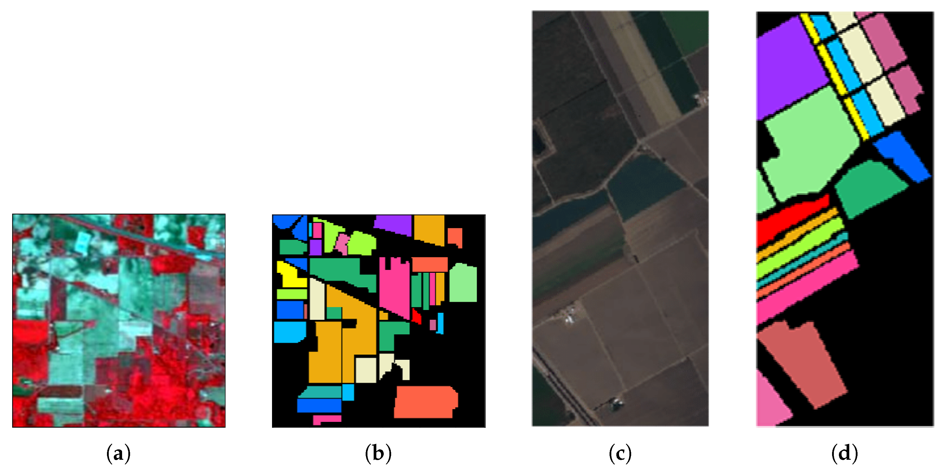
We complete a set of experiments on a pair of datasets collected by the same hyperspectral sensor. The reason for this selection is that different hyperspectral sensors have significant spectral gaps in hyperspectral imaging due to differences in wavelength range and spectral resolution. Our choice of pair datasets acquired by the same hyperspectral sensor can maintain greater consistency in the physical meaning of the spectra. So, we select four public hyperspectral datasets, including Indian Pines (IP), Salinas (SA), Pavia Center (PC), and Pavia University (PU). The false color images and the corresponding groundtruth maps are shown in Figure 8 and Figure 9, respectively. According to the hyperspectral sensor type of collecting data, we divide them into two groups, A and B. Each group has two datasets to form a pair of training set and testing set. 
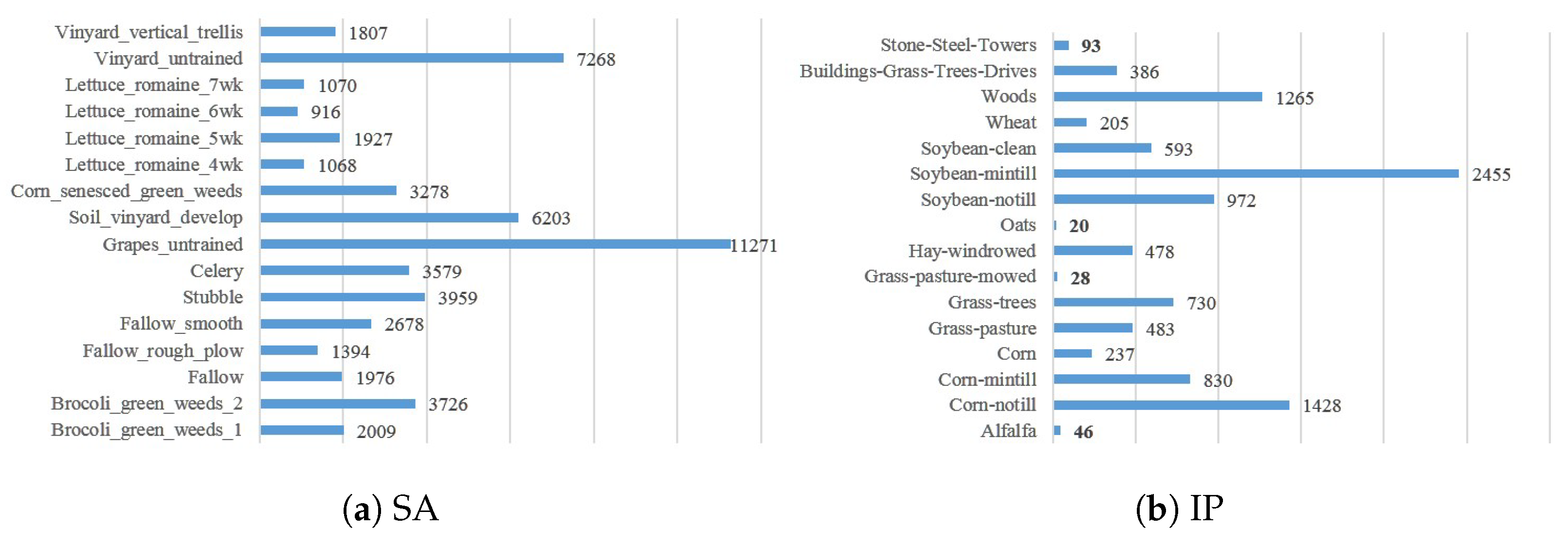
Table 1 shows the detailed information of these four datasets. In addition, the name of categories and the corresponding number of samples of these two groups are shown in
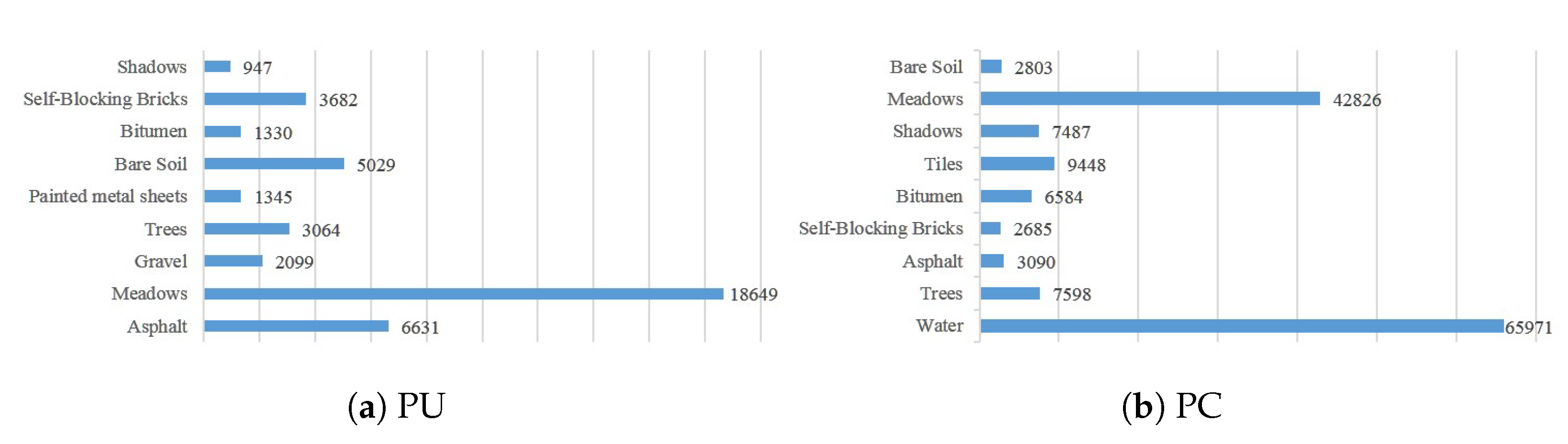
 Figure 10 and Figure 11, separately.
For HSI classification across different datasets, it is important to choose the appropriate combination of training and test sets. We split the selected datasets into the following 2 groups.
Group A: The Indian Pines dataset and the Salinas dataset. Both datasets were acquired by the AVIRIS sensor. To keep the input dimension of spectral consistent, we removed the last four bands from the Salinas dataset. Both of these two datasets has 16 different categories, but there are too few samples of some categories in this dataset, which will cause serious problems of category imbalance, so we exclude categories with less than 200 samples, including Alfalfa, Grass-pasture-mowed, Oats and Stone-Steel-Towers. The final selected categories of the training and testing sets are listed in Table 2. We design two cases of training and testing set as follows:
  • Case 1: IP-SA
    Training Set—Indian Pines dataset with 12 categories.
    Testing Set—Salinas dataset 16 categories.
  • Case 2: SA-IP
    Training Set—Salinas dataset with 12 categories.
    Testing Set—Indian Pines dataset 16 categories.
Group B: The Pavia Center dataset and the Pavia University dataset. Both datasets were acquired by the ROSIS sensor. To keep the input dimension of spectral consistent, we remove the last band from the Pavia University dataset. Each dataset covers 9 different categories, but 6 categories are the same between these two datasets. In order to keep the categories of training and testing set disjoint, we choose 5 categories of Pavia Center dataset and 6 categories of Pavia University dataset to form the combinations, which listed in Table 3. We design two cases of training and testing set as follows:
  • Case 3: PU-PC
    Training Set—Pavia University dataset with 6 categories.
    Testing Set—Pavia Center dataset 5 categories.
  • Case 4: PC-PU
    Training Set—Pavia Center dataset with 5 categories.
    Testing Set—Pavia University dataset 6 categories.
Besides, considering that the hyperspectral images of two different regions actually collected are likely to have duplicate land-cover categories, so we also perform experiments on dataset-pairs with duplicate categories in another two cases as follows:
  • Case 5: PU’-PC’
    Training Set—Pavia University dataset with 9 categories.
    Testing Set—Pavia Center dataset 9 categories.
  • Case 6: PC’-PU’
    Training Set—Pavia Center dataset with 9 categories.
    Testing Set—Pavia University dataset 9 categories.

5.2. Evaluation Metric

The datasets we use are small and have few categories, so the search space at evaluation time is restricted to the test categories ( Y TE ) in the experimental setting. We employ the average per-class top-k accuracy as the metric and list top-1 accuracy and top-3 accuracy as the results. We average the correct predictions for each category before dividing their cumulative sum of the number of classes, the average per-class top-k accuracy is defined as the following way:
a c c t o p - k = 1 | | Y TE | | c = 1 | | Y TE | | m c test labels
where m c is the number of correct predictions of top-k rank in c.

5.3. Implementation Details

5.3.1. Visual Embeddings

We obtain visual embeddings from the aforementioned HSI classification models. For each combination of training and testing sets, we retrain and optimal the model for each training set and save its model parameters as a pre-trained model. We finally load the pre-trained model without the softmax layer of the original classifier and get the visual embeddings.
For the bands-grouping RNN, we group 10 bands for each time step. The hidden layer units of RNN is set to 256, and the size of latter fully-connected layer is set to 128. For the ResNet18, it contains 17 convolutional layers and a fully connected layer. The size of spatial region for each pixel is set to 28 × 28 × 3 , and the last fully connected layer output a 512-dimensional visual feature vector. For the SSAN, the size of spatial region for each pixel is set to 28 × 28 × 3 , and the output of fully connected layer is 1024-dimensional. In addition, we employ L2 regularization and a dropout parameter set to 0.4 to avoid overfitting.
These three methods also have some common parameters in training, the batch size of the pre-training stage is set to 256 and the learning rate is 0.001.

5.3.2. Semantic Label Embeddings
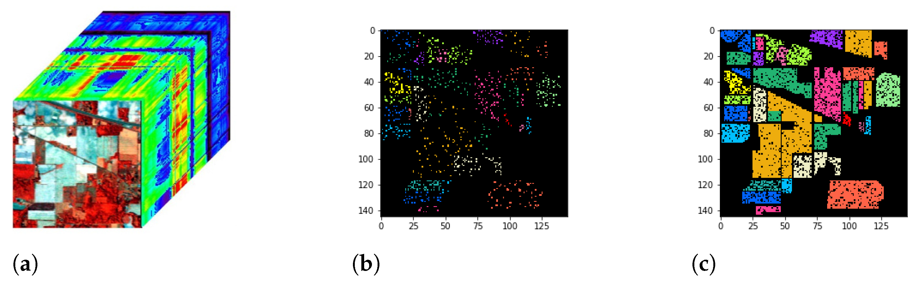
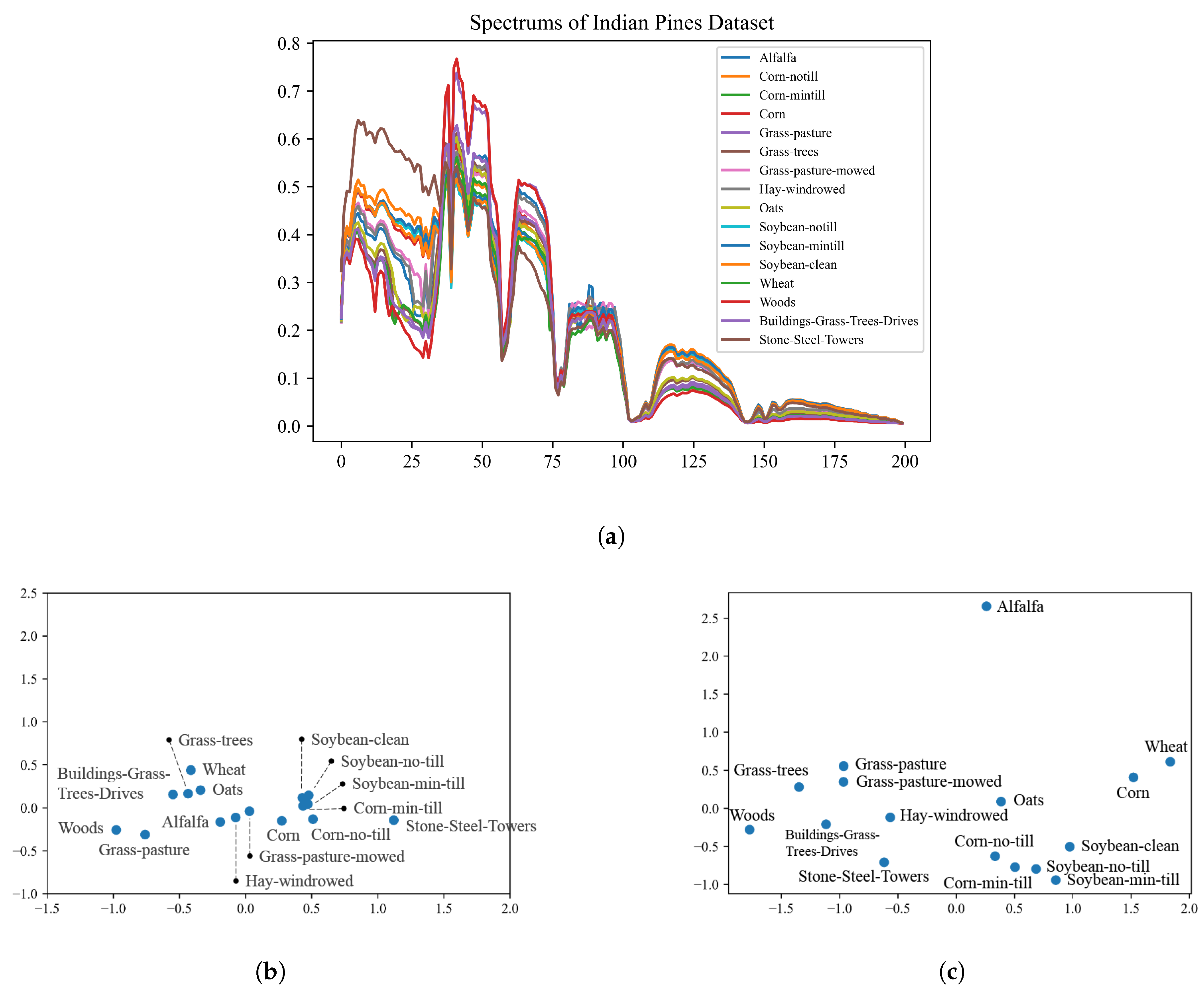
As illustrated in Figure 12, first of all, Figure 12a indicates that some categories in Indian Pines dataset are hard to classify in the origin spectral dimension, especially “Soybean-clean”, “Soybean-no-till”, “Soybean-min-till” and “Corn-min-till” according to 
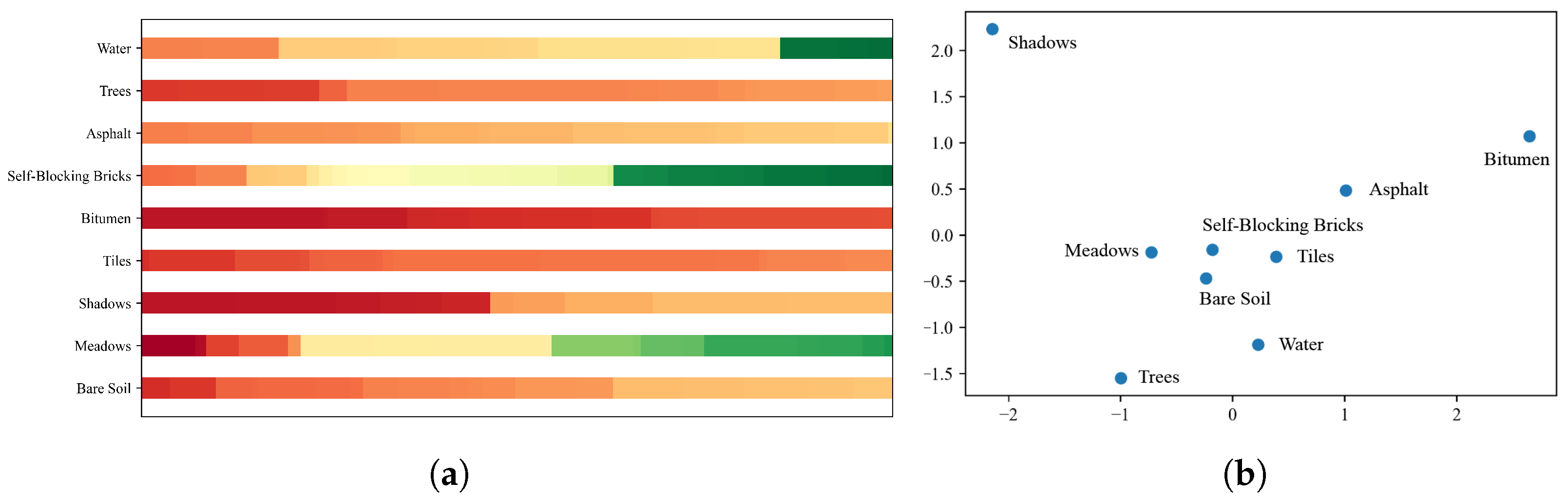
Figure 12b. Relatively speaking, as PCA 2D projection of word2vec vectors in Figure 12c, it shows that label semantic representations have good separability of categories. It also proves the effectiveness of word2vec vectors.
In addtion, many categories of names in the HSI dataset are composed of multiple words, so we load and average the word vectors corresponding to each category. Secondly, not all words of category names can be found in this corpus. Thus, we have modified the names of categories slightly without violating the original meaning. For instance, “Lettuce_romanine_4wk” refers to the lettuce that grows in the fourth week, but “4wk” is not a word, so we change it to “Lettuce_romanine_4”. The same operation applies to other categories.

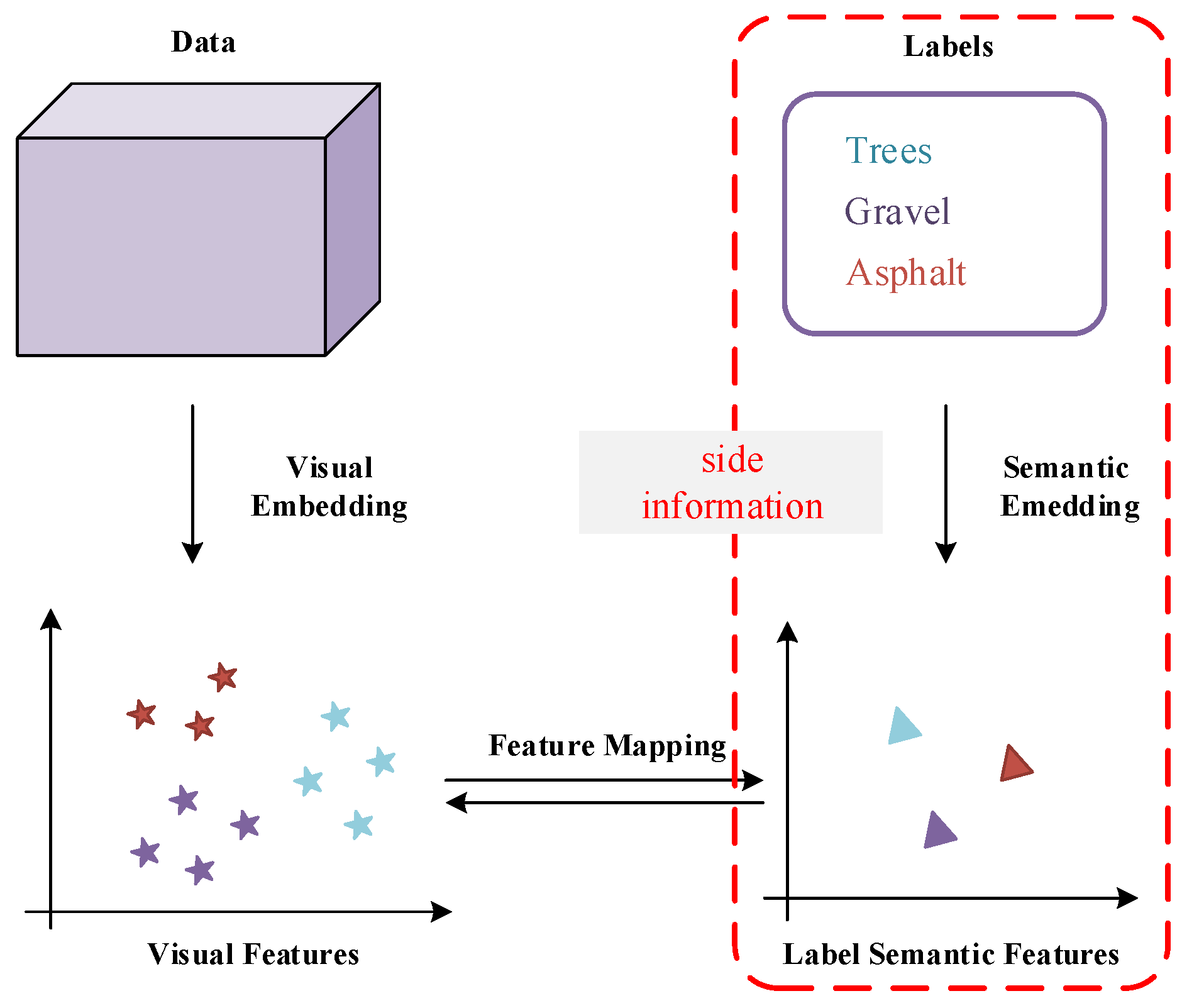
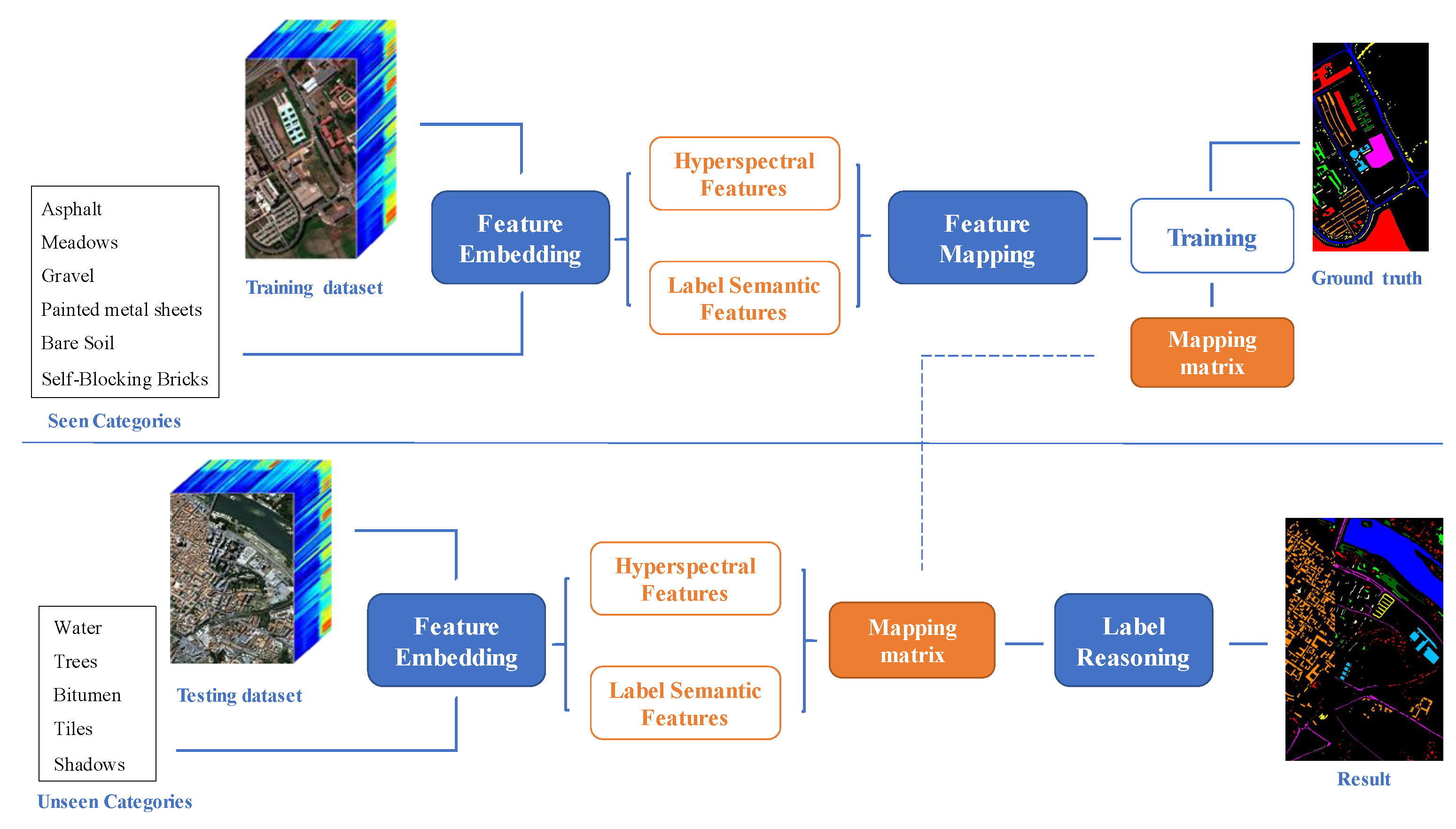
5.3.3. Visual-Semantic Alignment

Many classic zero-shot learning methods make use of category attributes provided by the public dataset, but there is no corresponding attributes data in the hyperspectral dataset. Therefore, we choose some models that only used word embeddings as the category reference data.
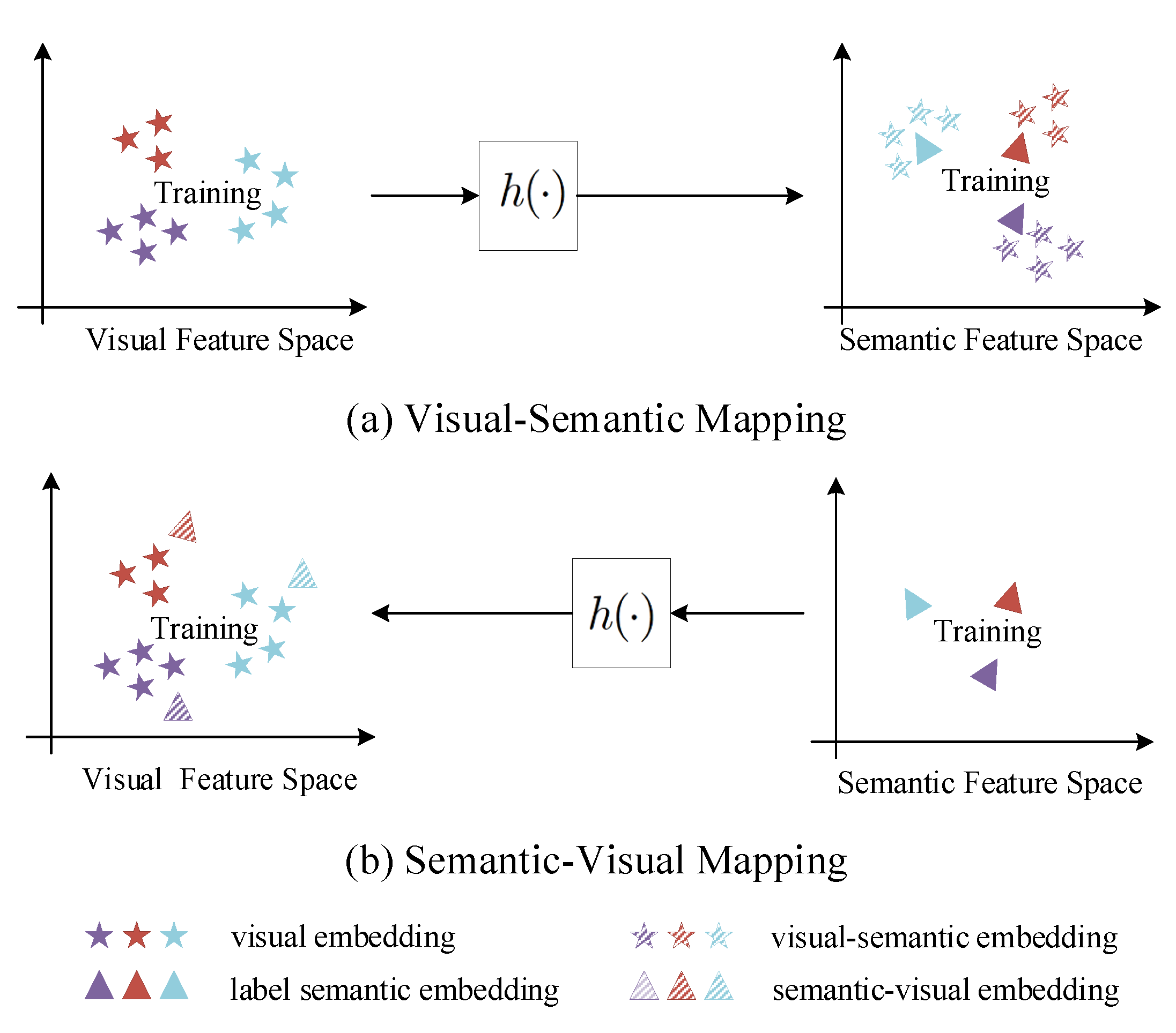
The selected comparative methods are DeVise, WLE, SAE, DEM and RN. All of them have been briefly introduced previously. Specifically, Word2Vec Label Embedding (WLE) is a variant of Attribute Label Embedding (ALE) model that uses word2vec instead of attributes. In these methods, DeVise and WLE align two parts of embeddings in the semantic space, and DEM and relation network are mapping the label semantic embeddings to the visual space. Moreover, SAE can be applied in both two space. The parameter settings are listed in Table 4.

5.4. Analysis of Experimental Results

We take the training and testing set in six cases with their selected categories, and report the experimental results using visual features obtained from bands-grouping RNN, ResNet18 and SSAN, respectively. Table 5 list results on GroupA datasets with case 1 and case 2 (IP and SA), Table 6 present the results on GroupB datasets with case 3 and case 4 (PU and PC), and Table 7 shows results on GroupB datasets with case 5 and case 6 (PU’ and PC’). The reports list the average results of 5 runs.
The comparison of experimental results using different feature extraction networks show that the source of visual embeddings has a considerable effect on the experimental results. The results indicate that the performance of SSAN which extracts joint spatial-spectral features is better than both the bands-grouping RNN which only focuses on the spectral feature and ResNet18 which concentrates on the spatial information. It is consistent with the trend in ordinary hyperspectral classification methods. For Group A, this is because IP and SA are collected from rural areas which mostly covered with crops, and the crops usually have a homogeneous distribution in the spatial domain. In contrast, Group B datasets have intricate distribution spatially. PC and PU provide data from the urban area, some category distributions here are decentralized, and some are mixed together. The advantage of HSI is the rich spectral information, also the introduction of complex spatial distribution has a positive impact on the performance of the classification or recognition task. Therefore, the superiority of hyperspectral data can be brought into play only by combining and fully mining the spectral and spatial information.
As we can observe, Group A is underperformed, especially the IP-SA case. The results of SAE and WLE with visual feature embedding under bands-grouping RNN are even nearly close to random classification performance. The poor performance may be caused by the reason that the categories in Group A mainly are crops, some of which only have a slight difference in terms of the name. For example, “Brocoli_green_weeds_1” and “Brocoli_green_weeds_2” in Salinas dataset, or “Soybean-no till”, “Soybean-min till” and “Soybean-clean” in Indian Pines dataset. They belong to the same type of land cover, but they have different spectra in hyperspectral data because they are under different conditions. Therefore, in the HSI data set, they are usually distinguished by adding other words or numbers. In zero-shot learning, we employ label semantic representation as side information, but for these categories which are only slightly different in name, they are difficult to distinguish semantically. It has a certain negative impact on classification performance.
Focusing on case 3 and case 4 of Group B (see Table 6), it can be noticed that only the results of the WLE and RN perform beyond the random classification performance in the PU-PC case. This is in stark contrast to the results of another case PC-PU, in which all zero-shot learning methods perform better. The huge difference between the number of labeled samples for training and testing comes to the first reason for this situation. It can be seen in Table 3, the PC dataset has 91,775 labeled samples while the PU dataset only has 36,817 in case 3 and case 4. The second reason is the unbalanced categories. Both of them have severely uneven data distribution. For example, the number of “Waters” in the PC dataset is 65,571 and “Meadows” has 18,449 samples in PU dataset while the other categories only have a few thousand. Group A has a similar situation. Besides, Group B covers the scene captured from the urban area, where most of the categories have a scattered and complex spatial distribution.
The “ V / S ” item in the tables indicate the choice of embedding space. Among all the zero-shot learning methods, the results in SAE are unsatisfactory, and several items of accuracy are even lower than the performance of random prediction. It suggests that there is no linear relationship between the visual feature embedding and the label semantic embedding. Besides, the performance of DeVise and WLE also prove that, both of which employ bi-linear compatibility function to connect the visual feature embedding and the label semantic embedding. So this kind of method cannot generalized well in the HSI classification task. Through these comparative experiments, it can be found that the “ S V ” method shows better results no matter under different visual feature extraction models or in different combinations of training and testing datasets, especially RN. It implies that treat visual space as an embedding space is a better choice for the application of zero-shot learning in HSI classification.
Case 5 and case 6 where the training set and the testing set shared some categories are attempts for generalized zero-shot learning. Table 7 shows the experimental results. Compared with previous experiments, the top-k accuracy has no significant improvement with the existence of common categories. There are two main reasons. First of all, both datasets have 9 categories, but their distribution of each category is visibly different, even the same categories in PC or PU has a significant difference in distribution. For example, the entire PC dataset contains 148,152 labeled samples and the PU dataset contains 42,776 labeled samples in total. What’s more, as shown in Figure 11, “Meadows” has 18,649 labeled samples in the PU dataset but has 42,826 in the PC dataset.“Self-Blocking Bricks” is the category with the fewest samples in the PC dataset, and there are only 2685 samples, but it ranks fifth in the number of samples in the PU dataset, with 3682 samples. Secondly, it is worth mentioning that the spectra of the same land-cover may not be fully consistent. The spectral curves of the same type of land-cover in the same dataset may have a certain range of fluctuation due to the spatial distribution or occlusion. Moreover, for these two datasets collected by the same sensor, the differences in the imaging environment, such as different weather conditions or lighting effects, may cause some variations in the spectrum of the same category. These also have a certain interference on the performance of classification. Besides, the experimental result of case 5 and case 6 are also consistent with the trends of the previous experiments.
In addition, in order to prove the positive effect of generalized zero-shot learning, we add a comparison with the ordinary hyperspectral classification in cases 5 and case 6, Figure 13 shows the top-1 accuracy of each comparative methods. As we can see, the DEM and RN perform more robust and superior.

6. Conclusions and Discussion

6.1. Conclusions

In this work, we introduce a new paradigm of HSI classification training and testing the classifier on different datasets. It breaks through the traditional HSI classification paradigm of dividing training and testing data on the same data cube. Considering the differences in the acquisition, preprocessing, and spectral resolution of different hyperspectral sensors, we select a pair of hyperspectral datasets captured from the same imaging sensor forming the training set and the testing set, respectively. Once trained, the classifier can be applied to any HSI data collected by the same hyperspectral sensor, as long as we know the contained categories, and it does not require a re-training process.
Because of the difference in the imaging scene, there is always a gap in the categories of different HSI datasets. To narrow the gap between the training set and the testing set of this task, we employ label semantic representations as side information. It can help establish connections between seen and unseen categories. Then, it learns the relationships between the visual features of hyperspectral data and semantic features of labels by feature mapping. Finally, the learned mapping is transferred to the testing data, and we derive the final label by similarity metric in label reasoning. In this work, we select word2vec as the label embedding tool, and we compare three hyperspectral feature extraction models. Moreover, we mainly analyze zero-shot learning methods, including SAE, ALE, DeVise, DEM, and RN, with different visual-semantic alignment strategies. Experimental results show the potential of our scheme for HSI classification across different datasets.

6.2. Discussion

The hyperspectral image dataset covers a scene with various land-cover categories, and the spatial distributions usually are complex and diverse. Domain shift in both spatial and spectral is the main issue of this task. For example, in rural area datasets such as Indian Pines and Salinas, the crop categories may include different growing periods of the same crop (as “Soybean no-till”, “Soybean min-till” and “Soybean clean” in Indian Pines). Despite their spectral differences, it is still difficult to distinguish these categories semantically. Another is urban area datasets such as Pavia Center and Pavia University. Their category distribution is very scattered, and the distribution of the same category in different datasets is also significantly different. This is also part of the reasons for poor classification results currently. Besides, there are very few publicly available hyperspectral datasets, and datasets from the same sensor are even rarer, which all pose a huge challenge for dealing with the hyperspectral image classification task across datasets. However, starting from the proposed solution, many improvements and extensions are possible to improve the performance. It still can be a future trend.
References yes

Author Contributions

All the authors made significant contributions to the work. E.P. and Y.M. conceived and designed the research and performed the experiments. E.P. and F.F. analyzed the results and wrote the manuscript. X.M. and J.H. provided insightful advices to this work and revised the manuscript. All authors have read and agreed to the published version of the manuscript.

Funding

This research was funded by the National Natural Science Foundation of China under Grant 61805181, Grant 61705170 and Grant 61903279.

Institutional Review Board Statement

Not applicable.

Informed Consent Statement

Not applicable.

Data Availability Statement

Public hyperspectral datasets are acquried from http://www.ehu.eus/ccwintco/index.php?title=Hyperspectral_Remote_Sensing_Scenes (accessed on 1 April 2021).

Conflicts of Interest

The authors declare no conflict of interest.

References

  1. Li, S.; Song, W.; Fang, L.; Chen, Y.; Ghamisi, P.; Benediktsson, J.A. Deep Learning for Hyperspectral Image Classification: An Overview. IEEE Trans. Geosci. Remote Sens. 2019, 57, 6690–6709. [Google Scholar] [CrossRef] [Green Version]
  2. Hu, J.; Peng, J.; Zhou, Y.; Xu, D.; Zhao, R.; Jiang, Q.; Fu, T.; Wang, F.; Shi, Z. Quantitative Estimation of Soil Salinity Using UAV-Borne Hyperspectral and Satellite Multispectral Images. Remote Sens. 2019, 11, 736. [Google Scholar] [CrossRef] [Green Version]
  3. Jin, X.; Jie, L.; Wang, S.; Qi, H.J.; Li, S.W. Classifying Wheat Hyperspectral Pixels of Healthy Heads and Fusarium Head Blight Disease Using a Deep Neural Network in the Wild Field. Remote Sens. 2018, 10, 395. [Google Scholar] [CrossRef] [Green Version]
  4. Ghamisi, P.; Yokoya, N.; Li, J.; Liao, W.; Liu, S.; Plaza, J.; Rasti, B.; Plaza, A. Advances in hyperspectral image and signal processing: A comprehensive overview of the state of the art. IEEE Geosci. Remote Sens. Mag. 2017, 5, 37–78. [Google Scholar] [CrossRef] [Green Version]
  5. Li, Y.; Ma, J.; Zhang, Y. Image retrieval from remote sensing big data: A survey. Inf. Fusion 2021, 67, 94–115. [Google Scholar] [CrossRef]
  6. Li, Y.; Chen, W.; Zhang, Y.; Tao, C.; Xiao, R.; Tan, Y. Accurate cloud detection in high-resolution remote sensing imagery by weakly supervised deep learning. Remote Sens. Environ. 2020, 250, 112045. [Google Scholar] [CrossRef]
  7. Paoletti, M.E.; Haut, J.M.; Plaza, J.; Plaza, A. Deep and Dense Convolutional Neural Network for Hyperspectral Image Classification. Remote Sens. 2018, 10, 1454. [Google Scholar] [CrossRef] [Green Version]
  8. Jiang, J.; Ma, J.; Chen, C.; Wang, Z.; Cai, Z.; Wang, L. SuperPCA: A superpixelwise PCA approach for unsupervised feature extraction of hyperspectral imagery. IEEE Trans. Geosci. Remote Sens. 2018, 56, 4581–4593. [Google Scholar] [CrossRef] [Green Version]
  9. Chang, C.I. Hyperspectral Imaging: Techniques for Spectral Detection and Classification; Springer Science & Business Media: New York, NY, USA, 2003; Volume 1. [Google Scholar]
  10. Zhang, L.; Zhang, L.; Du, B. Deep learning for remote sensing data: A technical tutorial on the state of the art. IEEE Geosci. Remote Sens. Mag. 2016, 4, 22–40. [Google Scholar] [CrossRef]
  11. Deng, J.; Dong, W.; Socher, R.; Li, L.; Li, K.; Feifei, L. Imagenet: A large-scale hierarchical image database. In Proceedings of the IEEE Conference on Computer Vision and Pattern Recognition, Miami, FL, USA, 20–25 June 2009; pp. 248–255. [Google Scholar]
  12. Pan, B.; Shi, Z.; Xu, X. MugNet: Deep learning for hyperspectral image classification using limited samples. ISPRS J. Photogramm. Remote Sens. 2018, 145, 108–119. [Google Scholar] [CrossRef]
  13. Fang, L.; Liu, G.; Li, S.; Ghamisi, P.; Benediktsson, J.A. Hyperspectral Image Classification With Squeeze Multibias Network. IEEE Trans. Geosci. Remote Sens. 2019, 57, 1291–1301. [Google Scholar] [CrossRef]
  14. Peng, C.; Tian, T.; Chen, C.; Guo, X.; Ma, J. Bilateral attention decoder: A lightweight decoder for real-time semantic segmentation. Neural Netw. 2021, 137, 188–199. [Google Scholar] [CrossRef]
  15. Shi, C.; Pun, C.M. Multiscale superpixel-based hyperspectral image classification using recurrent neural networks with stacked autoencoders. IEEE Trans. Multimed. 2019, 22, 487–501. [Google Scholar] [CrossRef]
  16. Peng, C.; Ma, J. Semantic segmentation using stride spatial pyramid pooling and dual attention decoder. Pattern Recognit. 2020, 107, 107498. [Google Scholar] [CrossRef]
  17. Peng, C.; Zhang, K.; Ma, Y.; Ma, J. Cross Fusion Net: A Fast Semantic Segmentation Network for Small-Scale Semantic Information Capturing in Aerial Scenes. IEEE Trans. Geosci. Remote Sens. 2021. [Google Scholar] [CrossRef]
  18. Liang, J.; Zhou, J.; Qian, Y.; Wen, L.; Bai, X.; Gao, Y. On the Sampling Strategy for Evaluation of Spectral-Spatial Methods in Hyperspectral Image Classification. IEEE Trans. Geosci. Remote Sens. 2017, 55, 862–880. [Google Scholar] [CrossRef] [Green Version]
  19. Hänsch, R.; Ley, A.; Hellwich, O. Correct and still wrong: The relationship between sampling strategies and the estimation of the generalization error. In Proceedings of the IEEE International Geoscience and Remote Sensing Symposium, Fort Worth, TX, USA, 23–28 July 2017; pp. 3672–3675. [Google Scholar]
  20. Paoletti, M.; Haut, J.; Plaza, J.; Plaza, A. Deep learning classifiers for hyperspectral imaging: A review. ISPRS J. Photogramm. Remote Sens. 2019, 158, 279–317. [Google Scholar] [CrossRef]
  21. Baumgardner, M.F.; Biehl, L.L.; Landgrebe, D.A. 220 Band AVIRIS Hyperspectral Image Data Set: June 12, 1992 Indian Pine Test Site 3; Purdue University Research Repository: West Lafayette, Indiana, 2015. [Google Scholar] [CrossRef]
  22. Plaza, A.; Martínez, P.; Plaza, J.; Pérez, R. Dimensionality reduction and classification of hyperspectral image data using sequences of extended morphological transformations. IEEE Trans. Geosci. Remote Sens. 2005, 43, 466–479. [Google Scholar] [CrossRef] [Green Version]
  23. Lee, H.; Eum, S.; Kwon, H. Cross-Domain CNN for Hyperspectral Image Classification. In Proceedings of the IGARSS 2018—2018 IEEE International Geoscience and Remote Sensing Symposium, Valencia, Spain, 22–27 July 2018; pp. 3627–3630. [Google Scholar] [CrossRef] [Green Version]
  24. Geng, J.; Ma, X.; Jiang, W.; Hu, X.; Wang, D.; Wang, H. Cross-Scene Hyperspectral Image Classification Based on Deep Conditional Distribution Adaptation Networks. In Proceedings of the IGARSS 2019—2019 IEEE International Geoscience and Remote Sensing Symposium, Yokohama, Japan, 28 July–2 August 2019; pp. 716–719. [Google Scholar] [CrossRef]
  25. Shen, J.; Cao, X.; Li, Y.; Xu, D. Feature Adaptation and Augmentation for Cross-Scene Hyperspectral Image Classification. IEEE Geosci. Remote Sens. Lett. 2018, 15, 622–626. [Google Scholar] [CrossRef]
  26. Changpinyo, S.; Chao, W.L.; Sha, F. Predicting Visual Exemplars of Unseen Classes for Zero-Shot Learning. In Proceedings of the IEEE International Conference on Computer Vision, Venice, Italy, 22–29 October 2017; pp. 3496–3505. [Google Scholar] [CrossRef] [Green Version]
  27. Fu, Y.; Xiang, T.; Jiang, Y.G.; Xue, X.; Sigal, L.; Gong, S. Recent advances in zero-shot recognition: Toward data-efficient understanding of visual content. IEEE Signal Process. Mag. 2018, 35, 112–125. [Google Scholar] [CrossRef]
  28. Annadani, Y.; Biswas, S. Preserving Semantic Relations for Zero-Shot Learning. In Proceedings of the IEEE Conference on Computer Vision and Pattern Recognition, Salt Lake City, UT, USA, 18–22 June 2018; pp. 7603–7612. [Google Scholar] [CrossRef] [Green Version]
  29. Xian, Y.; Lampert, C.H.; Schiele, B.; Akata, Z. Zero-Shot Learning—A Comprehensive Evaluation of the Good, the Bad and the Ugly. IEEE Trans. Pattern Anal. Mach. Intell. 2019, 41, 2251–2265. [Google Scholar] [CrossRef] [PubMed] [Green Version]
  30. Lampert, C.H.; Nickisch, H.; Harmeling, S. Learning to detect unseen object classes by between-class attribute transfer. In Proceedings of the IEEE Conference on Computer Vision and Pattern Recognition, Miami, FL, USA, 20–25 June 2009; pp. 951–958. [Google Scholar] [CrossRef]
  31. Romera-Paredes, B.; Torr, P. An embarrassingly simple approach to zero-shot learning. In Proceedings of the 32nd International Conference on Machine Learning, Lille, France, 7–9 July 2015; pp. 2152–2161. [Google Scholar]
  32. Wang, W.; Zheng, V.W.; Yu, H.; Miao, C. A survey of zero-shot learning: Settings, methods, and applications. ACM Trans. Intell. Syst. Technol. 2019, 10, 13. [Google Scholar] [CrossRef]
  33. Lampert, C.H.; Nickisch, H.; Harmeling, S. Attribute-based classification for zero-shot visual object categorization. IEEE Trans. Pattern Anal. Mach. Intell. 2013, 36, 453–465. [Google Scholar] [CrossRef] [PubMed]
  34. Frome, A.; Corrado, G.S.; Shlens, J.; Bengio, S.; Dean, J.; Ranzato, M.; Mikolov, T. Devise: A deep visual-semantic embedding model. In Proceedings of the 26th International Conference on Neural Information Processing Systems, Lake Tahoe, NV, USA, 5–8 December 2013; pp. 2121–2129. [Google Scholar]
  35. Wang, W.; Pu, Y.; Verma, V.K.; Fan, K.; Zhang, Y.; Chen, C.; Rai, P.; Carin, L. Zero-shot learning via class-conditioned deep generative models. In Proceedings of the AAAI Conference on Artificial Intelligence, New Orleans, LA, USA, 2–7 February 2017. [Google Scholar]
  36. Griffiths, T.L.; Steyvers, M.; Tenenbaum, J.B. Topics in semantic representation. Psychol. Rev. 2007, 114, 211. [Google Scholar] [CrossRef] [Green Version]
  37. Levy, O.; Goldberg, Y. Dependency-based word embeddings. In Proceedings of the 52nd Annual Meeting of the Association for Computational Linguistics, Baltimore, MD, USA, 23–24 June 2014; pp. 302–308. [Google Scholar]
  38. Li, J.; Chen, X.; Hovy, E.; Jurafsky, D. Visualizing and Understanding Neural Models in NLP. In Proceedings of the North American Chapter of the Association for Computational Linguistics: Human Language Technologies, San Diego, CA, USA, 12–17 June 2016; pp. 681–691. [Google Scholar]
  39. Mikolov, T.; Chen, K.; Corrado, G.; Dean, J. Efficient estimation of word representations in vector space. arXiv 2013, arXiv:1301.3781. [Google Scholar]
  40. Chung, Y.A.; Wu, C.C.; Shen, C.H.; Lee, H.Y.; Lee, L.S. Audio word2vec: Unsupervised learning of audio segment representations using sequence-to-sequence autoencoder. arXiv 2016, arXiv:1603.00982. [Google Scholar]
  41. Luan, Y.; Watanabe, S.; Harsham, B. Efficient learning for spoken language understanding tasks with word embedding based pre-training. In Proceedings of the 16th Annual Conference of the International Speech Communication Association, Dresden, Germany, 6–10 September 2015. [Google Scholar]
  42. Zhang, X.; Wei, F.; Zhou, M. HIBERT: Document Level Pre-training of Hierarchical Bidirectional Transformers for Document Summarization. In Proceedings of the 57th Annual Meeting of the Association for Computational Linguistics, Florence, Italy, 28 July–2 August 2019; pp. 5059–5069. [Google Scholar]
  43. Li, C.; Ma, Y.; Mei, X.; Liu, C.; Ma, J. Hyperspectral image classification with robust sparse representation. IEEE Geosci. Remote Sens. Lett. 2016, 13, 641–645. [Google Scholar] [CrossRef]
  44. Zhong, Z.; Li, J.; Ma, L.; Jiang, H.; Zhao, H. Deep residual networks for hyperspectral image classification. In Proceedings of the IEEE International Geoscience and Remote Sensing Symposium, Fort Worth, TX, USA, 23–28 July 2017; pp. 1824–1827. [Google Scholar]
  45. He, K.; Zhang, X.; Ren, S.; Sun, J. Deep residual learning for image recognition. In Proceedings of the IEEE Conference on Computer Vision and Pattern Recognition, Las Vegas, NV, USA, 27–30 June 2016; pp. 770–778. [Google Scholar]
  46. Mei, X.; Pan, E.; Ma, Y.; Dai, X.; Huang, J.; Fan, F.; Du, Q.; Zheng, H.; Ma, J. Spectral-Spatial Attention Networks for Hyperspectral Image Classification. Remote Sens. 2019, 11, 963. [Google Scholar] [CrossRef] [Green Version]
  47. Ma, X.; Wang, H.; Wang, J. Semisupervised classification for hyperspectral image based on multi-decision labeling and deep feature learning. ISPRS J. Photogramm. Remote Sens. 2016, 120, 99–107. [Google Scholar] [CrossRef]
  48. Mou, L.; Ghamisi, P.; Zhu, X.X. Deep recurrent neural networks for hyperspectral image classification. IEEE Trans. Geosci. Remote Sens. 2017, 55, 3639–3655. [Google Scholar] [CrossRef] [Green Version]
  49. Xu, Y.; Zhang, L.; Du, B.; Zhang, F. Spectral-Spatial Unified Networks for Hyperspectral Image Classification. IEEE Trans. Geosci. Remote Sens. 2018, 56, 5893–5909. [Google Scholar] [CrossRef]
  50. Pan, E.; Mei, X.; Wang, Q.; Ma, Y.; Ma, J. Spectral-spatial classification for hyperspectral image based on a single GRU. Neurocomputing 2020, 387, 150–160. [Google Scholar] [CrossRef]
  51. Akata, Z.; Perronnin, F.; Harchaoui, Z.; Schmid, C. Label-Embedding for Image Classification. IEEE Trans. Pattern Anal. Mach. Intell. 2016, 38, 1425–1438. [Google Scholar] [CrossRef] [Green Version]
  52. Kodirov, E.; Xiang, T.; Gong, S. Semantic autoencoder for zero-shot learning. In Proceedings of the IEEE Conference on Computer Vision and Pattern Recognition, Honolulu, HI, USA, 21–26 July 2017; pp. 4447–4456. [Google Scholar] [CrossRef] [Green Version]
  53. Mikolov, T.; Sutskever, I.; Chen, K.; Corrado, G.S.; Dean, J. Distributed representations of words and phrases and their compositionality. In Proceedings of the 26th International Conference on Neural Information Processing Systems, Lake Tahoe, NV, USA, 5–8 December 2013; pp. 3111–3119. [Google Scholar]
  54. Weston, J.; Bengio, S.; Usunier, N. Wsabie: Scaling up to large vocabulary image annotation. In Proceedings of the Twenty-Second International Joint Conference on Artificial Intelligence, Barcelona, Catalonia, Spain, 16–22 July 2011; pp. 2764–2770. [Google Scholar]
  55. Zhang, L.; Xiang, T.; Gong, S. Learning a deep embedding model for zero-shot learning. In Proceedings of the IEEE Conference on Computer Vision and Pattern Recognition, Honolulu, HI, USA, 21–26 July 2017; pp. 2021–2030. [Google Scholar]
  56. Sung, F.; Yang, Y.; Zhang, L.; Xiang, T.; Torr, P.H.; Hospedales, T.M. Learning to compare: Relation network for few-shot learning. In Proceedings of the IEEE Conference on Computer Vision and Pattern Recognition, Salt Lake City, UT, USA, 18–22 June 2018; pp. 1199–1208. [Google Scholar]
  57. Fauvel, M.; Tarabalka, Y.; Benediktsson, J.A.; Chanussot, J.; Tilton, J.C. Advances in Spectral-Spatial Classification of Hyperspectral Images. Proc. IEEE 2012, 101, 652–675. [Google Scholar] [CrossRef] [Green Version]
  58. Fauvel, M.; Benediktsson, J.A.; Chanussot, J.; Sveinsson, J.R. Spectral and spatial classification of hyperspectral data using SVMs and morphological profiles. IEEE Trans. Geosci. Remote Sens. 2008, 46, 3804–3814. [Google Scholar] [CrossRef] [Green Version]
Figure 1. (a) The HSI data cube of Indian Pines dataset [21], (b,c) illustrate the training set and the testing set under the random sampling strategy in HSI classification. The colored points represent the selected pixels. The training set consists of samples randomly selected with a fixed number in each categories, and the remaining samples form the testing set.
Remotesensing 13 01672 g001
Figure 2. Illustration of the basic framework of zero-shot learning. Visual features of training data and testing data are derived by visual embedding, Label semantic features are acquired by semantic embedding from seen and unseen labels as side information. The correspondence between semantic features and visual features is learned through feature mapping.
Remotesensing 13 01672 g002
Figure 3. (a) Label semantic distributions of the Pavia Center dataset, (b) PCA visualization of word embeddings in a two-dimensional space.
Remotesensing 13 01672 g003
Figure 4. Illustration of the whole scheme. In the training process, through feature embedding, the training data and the label of categories are embedded into the corresponding feature spaces to obtain hyperspectral features and label semantic features respectively. Then, a mapping matrix representing the correspondences between these features is learned by feature mapping. In the testing process, the learned mapping is transferred to the hyperspectral features and label semantic features of the testing data. At last, we derive the final label by label reasoning.
Remotesensing 13 01672 g004
Figure 5. Illustration of phase A, feature embedding, embed hyperspectral features and label semantic features into the corresponding feature spaces, respectively. Stars and triangles in the same color belong to the same category, and the gray one represents the unseen category.
Remotesensing 13 01672 g005
Figure 6. Illustration of phase B, feature mapping, including semantic-visual feature mapping and visual-semantic feature mapping. In this phase, a feature mapping model h ( · ) between two feature space is learned on the training set.
Remotesensing 13 01672 g006
Figure 7. Illustration of phase C, label reasoning. In this phase, the learned mapping h ( · ) is firstly applied to get the corresponding embedding, and then a similar metric g ( · ) is employed in the selected feature space to find the final label.
Remotesensing 13 01672 g007
Figure 8. (a) The false color image of the Indian Pines dataset [57], (b) The corresponding ground-truth map. (c) The false color image of the Salinas dataset [22], (d) The corresponding ground-truth map.
Remotesensing 13 01672 g008
Figure 9. (a) The false color image of the Pavia Center dataset [58], (b) The corresponding ground-truth map. (c) The false color image of the Pavia University dataset [58], (d) The corresponding ground-truth map.
Remotesensing 13 01672 g009
Figure 10. The name of categories and the corresponding number of labeled samples of datasets in Group A.
Remotesensing 13 01672 g010
Figure 11. The name of categories and the corresponding number of labeled samples of datasets in Group B.
Remotesensing 13 01672 g011
Figure 12. (a) Mean Spectrums curve of Indian Pines dataset, (b) PCA visualization of mean spectrums in 2-D, (c) PCA visualization of word2vec vectors in 2-D.
Remotesensing 13 01672 g012
Figure 13. The top-1 accuracy of the ordinary hyperspectral classification and the comparative zero-shot learning methods in case 5 PU’-PC’ and case 6 PC’-PU’.
Remotesensing 13 01672 g013
Table 1. Detailed information of four hyperspectral datasets. Indian Pines, Salinas, Pavia Center and Pavia University.
Group AGroup B
Indian PinesSalinasPavia CenterPavia University
SensorAVIRISAVIRISROSISROSIS
Spectral range400–2500400–2500430–860430–860
AreaIndianaCaliforniaPaviaPavia
Number of bands200204102103
Spatial size 145 × 145 512 × 217 1096 × 715 610 × 340
Number of classes161699
Table 2. The selected categories of Indian Pines dataset and Salinas dataset for Case 1 and Case 2.
No.Indian PinesSalinas
1Corn-no tillBrocoli_green_weeds_1
2Corn-min tillBrocoli_green_weeds_2
3CornFallow
4Grass-pastureFallow_rough_plow
5Grass-treesFallow_smooth
6Hay-windrowedStubble
7Soybean-no tillCelery
8Soybean-min tillGrapes_untrained
9Soybean-cleanSoil_Vinyard_develop
10WheatCorn_green_weeds
11WoodsLettuce_romaine_4
12Buildings-Grass-Trees-DrivesLettuce_romaine_5
13 Lettuce_romaine_6
14 Lettuce_romaine_7
15 Vinyard_untrained
16 Vinyard_vertical_trellis
Total10,06254,129
Table 3. The selected categories of Pavia Center dataset and Pavia University dataset for Case 3 and Case 4.
No.Pavia CenterPavia University
1WaterAsphalt
2Self-Blocking BricksMeadows
3BitumenGravel
4TilesTrees
5ShadowsPainted metal sheets
6 Bare Soil
Total91,77536,817
Table 4. Parameter configurations for comparative methods.
MethodsParameters
VisualBands-grouping RNNfeature dim = 128; the number of grouping bands = 10;
FeatureResNet18feature dim = 512; the spatial size = 28 × 28
EmbeddingSSANfeature dim = 1024; the spatial size = 28 × 28 ; dropout = 0.4
DeVisemargin = 0.1; learning_rate = 0.0001
ZeroWLElearning_rate = 0.001
-shotSAE λ = 100,000 ; learning_rate = 0.0001
LearningDEM λ = 0.0001 ; learning_rate = 0.00001
RNlearning_rate = 0.0001
Table 5. Classification performance of multiple comparative methods on GroupA datasets (Case 1 and Case 2) under different visual feature extraction models including the bands-grouping RNN, ResNet18, and SSAN. The best results are shown in red, the blue results represent the second-ranked and the third-ranked results are displayed in green.
AccModelV/SSA-IP (19)IP-SA (16)
BG-RNNResNet18SSANBG-RNNResNet18SSAN
Top1DeVise V S 13.8310.6715.8710.7711.4413.25
WLE V S 8.648.5711.606.9110.526.96
SAE V S 9.5410.5011.275.589.017.23
S V 10.088.1212.167.8112.667.35
DEM S V 17.4817.1122.6512.4112.038.28
RN S V 20.2113.7914.6013.5913.2514.25
Top3DeVise V S 28.2324.1431.6024.8723.8930.21
WLE V S 23.3321.9226.8816.6324.1821.79
SAE V S 23.9223.3726.7015.8316.1522.24
S V 29.1125.1125.5214.4914.5724.72
DEM S V 28.4231.5036.1025.4824.2928.68
RN S V 32.7628.4429.2830.2228.7838.09
Table 6. Classification performance of multiple comparative methods on GroupB datasets (Case 3 and Case 4) under different visual feature extraction models including the bands-grouping RNN, ResNet18, and SSAN. The best results are shown in red, the blue results represent the second-ranked and the third-ranked results are displayed in green.
AccModelV/SPU-PC (5)PC-PU (6)
BG-RNNResNet18SSANBG-RNNResNet18SSAN
Top1DeVise V S 12.9313.5517.9427.9420.4231.65
WLE V S 20.4417.8123.7228.2428.9137.44
SAE V S 9.596.345.4624.7921.6826.65
S V 10.567.037.1720.5019.5428.61
DEM S V 17.4717.4919.1024.8525.1541.07
RN S V 27.2221.3325.1631.3929.3933.43
Top3DeVise V S 23.8829.8445.1452.2738.0862.63
WLE V S 48.9748.3761.1756.7958.6868.77
SAE V S 26.2821.6223.4749.6440.7849.29
S V 22.0925.1928.6441.4237.3744.59
DEM S V 44.0545.3358.1953.7452.5277.39
RN S V 54.8559.8362.2168.1261.6367.85
Table 7. Classification performance of multiple comparative methods on GroupB datasets (Case 5 and Case 6) under different visual feature extraction models including the bands-grouping RNN, ResNet18, and SSAN. The best results are shown in red, the blue results represent the second-ranked and the third-ranked results are displayed in green.
AccModelV/SPU’-PC’ (9)PC’-PU’ (9)
BG-RNNResNet18SSANBG-RNNResNet18SSAN
Top1DeVise V S 10.348.1311.7512.5413.7613.52
WLE V S 12.5611.4914.2113.1218.4416.30
SAE V S 1.595.714.481.619.052.41
S V 4.887.468.482.296.723.36
DEM S V 13.2913.3222.1116.7117.4219.23
RN S V 19.7212.7321.5318.8218.0120.08
Top3DeVise V S 31.2227.8836.8031.5833.8435.65
WLE V S 37.0835.3439.2235.8339.1843.67
SAE V S 26.3726.6828.6032.1735.4434.17
S V 28.4127.9230.7026.6728.6337.89
DEM S V 39.0539.1347.5145.1444.4348.01
RN S V 41.3837.7545.1748.2446.2155.38
Publisher’s Note: MDPI stays neutral with regard to jurisdictional claims in published maps and institutional affiliations.

