Estimation of the Precipitable Water and Water Vapor Fluxes in the Coastal and Inland Cities of China Using MAX-DOAS

Abstract

Water vapor transport affects regional precipitation and climate change. The measurement of precipitable water (PW) and water vapor flux (WVF) is of great importance for the study of precipitation and water vapor transport. This study presented a new method of computing PW and estimating WVF using the water vapor vertical column density (VCD) and profile retrieved from multi-axis differential optical absorption spectroscopy (MAX-DOAS), combined with the European Centre for Medium-Range Weather Forecasts (ECMWF) ERA5 wind profiles. We applied our method to MAX-DOAS observations in the coastal (Qingdao) and inland (Xi’an) cities of China from June 2019 to May 2020 and compared the results to the ERA5 reanalysis datasets. Good agreement with ERA5 datasets was found; the correlation coefficient (r) of the PW and the zonal and meridional WVFs were r ≥ 0.92, r = 0.77, and r ≥ 0.89, respectively. The comparison results showed the feasibility and reliability of estimating PW and WVF using MAX-DOAS. Then, we analyzed the seasonal and diurnal climatology of the PW and WVFs in Qingdao and Xi’an. The results indicated that the seasonal and diurnal variations of the PW in the two cities were similar. The zonal water vapor transport of the two cities mainly involved eastward transport, Qingdao’s meridional water vapor mainly involved southward transport, and that of Xi’an mainly involved northward transport. The WVFs of the two cities were higher in the afternoon than in the morning, which may be related to wind speed. The results also indicated that the WVF transmitting belts appeared at around 2 and 1.4 km above the surface in Qingdao and around 2.8, 2.6, 1.6, and 1.0 km above the surface in Xi’an. Before precipitation, the WVF transmitting belt moved from near the ground to a high level, reaching its maximum at about 2 km, and the PW and meridional vertically integrated WVF increased. Finally, the sources and transports of water vapor during continuous precipitation and torrential rain were analyzed according to a 24 h backward trajectory. The air mass from the southeast accounted for more than 84% during continuous precipitation in Xi’an, while the air mass from the ocean accounted for more than 75% during torrential rain in Qingdao and was accompanied by a high-level ocean jet stream. As an optical remote sensing instrument, MAX-DOAS has the advantages of high spatiotemporal resolution, low cost, and easy maintenance. The application of MAX-DOAS to meteorological remote sensing provides a better method for evaluating the PW and WVF.

1. Introduction

Water vapor is the most important greenhouse gas in nature and plays a vital role in cloud formation, precipitation, and the atmospheric radiation budget [1]. Changes in atmospheric water vapor, especially tropospheric precipitable water (PW), directly affect the frequency of precipitation and provide resources for the study of climate change [2,3]. Water cycles also play an important role in global warming [4,5,6,7]. Tropospheric water vapor flux (WVF) is an important parameter in water cycles and an important factor affecting energy balance. Continuous observation of this parameter can reflect changes in the regional hydrological climate [8,9,10,11].

The water vapor concentration is greatly affected by transportation, local water vapor evaporation, and condensation [1]. To understand the climatic characteristics of regional precipitation and atmospheric water cycles, the measurement of PW and WVF is extremely important, especially in the lower troposphere. The water vapor concentration is usually higher in the lower atmosphere, and high concentrations are the most important for evaluating the condensation and transportation of water vapor.

The measurement methods of PW and WVF mainly include sounding, lidar, and global positioning system (GPS) detection. The radiosonde traditionally used for atmospheric water vapor analysis has a poor time resolution (12 h). Combining the water vapor profiles by Raman lidar measurements with the vertical wind profiles determined by wind lidar can estimate the atmospheric water vapor flux profiles within the convective boundary layer (CBL) [12,13]. GPS has been developed since 1990, and combined with wind radar, the WVF within the CBL can be measured [1]. Lidar and GPS systems have a high temporal and spatial resolution, but the lidar is expensive and difficult to maintain. The algorithm for the GPS system is also complicated. Therefore, developing a measuring method for PW and WVF with a low cost, simple algorithm, and easy maintenance is of great significance to the study of the water cycle.

Multi-axis differential optical absorption spectroscopy (MAX-DOAS) features a low cost, a simple instrument setup, a mature algorithm, and high spatiotemporal resolution; MAX-DOAS is also a widely used method for measuring the vertical column densities (VCDs) and profiles of trace gases (aerosol, NO₂, SO₂, HONO, HCHO, and CHOCHO) in the atmosphere [14,15,16,17,18,19,20]. MAX-DOAS is usually used in the study of atmospheric pollution, but there is a gap in meteorological research (PW and WVF). In recent years, measuring the atmospheric water vapor VCD and profile based on MAX-DOAS has been continuously studied [15,21,22,23,24,25,26,27], providing a new method for studying PW and WVF. Because of its simple structure, high temporal and spatial resolution, easy maintenance, and remote control, MAX-DOAS has great advantages over traditional atmospheric water vapor measuring instruments. Therefore, MAX-DOAS can serve as a useful tool for meteorological analysis and model verification. Moreover, MAX-DOAS can simultaneously retrieve multiple gases, such as pollutant gases (NO₂ and SO₂) and water vapor, which is very important for studying haze pollution.

The purpose of this study is to develop a new method for measuring PW and WVF using the MAX-DOAS instrument. Converting the water vapor VCD retrieved by MAX-DOAS into PW, and then combining the water vapor profile retrieved by PriAM with the European Centre for Medium-Range Weather Forecasts (ECMWF) ERA5 wind profile, the WVF could be calculated. This method was applied to the meteorological analysis of a typical inland city (Xi’an) and coastal city (Qingdao) in China. Xi’an is located in the southern part of the Guanzhong Plain, with an alluvial plain in the north and the Qinling Mountains in the south. Qingdao is located in the eastern part of Shandong Province, adjacent to the Yellow Sea. Xi’an has a warm temperate semi-humid continental monsoon climate and is affected by local circulation, such as valley circulation [28]. Qingdao has a maritime climate and is affected by the local circulation of sea and land winds [29]. Studying the PW and WVF of the inland and coastal cities in China will provide insight into the water cycle.

A detailed description of the experimental instrument and the new method for calculating PW and WVF are presented in Section 2. In Section 3, we analyze and discuss the seasonal and diurnal climatology of the PW and WVFs in Xi’an and Qingdao. In this section, we also analyze the variability of PW and WVF and water vapor transport before precipitation. A summary and conclusions are presented in Section 4.

2. Instruments and Methods

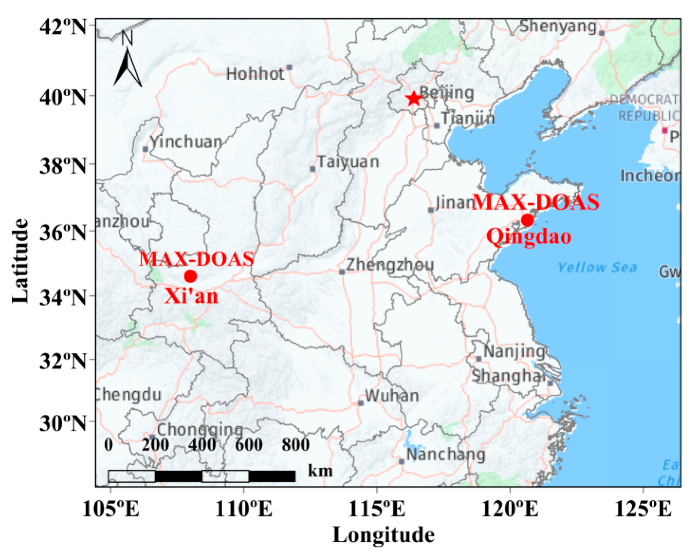
2.1. Overview of the Measurement Station

MAX-DOAS instruments developed by Anhui Institute of Optics and Fine Mechanics (AIOFM) of the Chinese Academy of Sciences were used for our experimental measurements [16,17,18,19,20,30,31].

MAX-DOAS mainly includes a spectrometer, a 360° controllable platform, a telescope, an optical fiber, a computer, and a monitoring camera (Figure 1). The 360° controllable platform, telescope, and monitoring camera were placed outdoors, and the rest of the equipment was placed indoors. The telescope, with an elevation angle range (EA) of 0°–90° and an azimuth angle range of 0°–360°, was controlled by the computer. Sunlight was collected by the telescope and then transmitted to the spectrometer through an optical fiber. The spectrometer was placed inside a temperature-controlled system set to 25 °C. The spectra were measured from 4:00 to 22:00 (UTC +8). The low-elevation spectrum at night was used to correct for the dark current. Integration of the spectrum acquisition was performed 100 times for every spectrum, and the integrational time was automatically adjusted according to the sunlight intensity. The specific parameters for MAX-DOAS retrieval are shown in

Table 1. Parameter settings for MAX-DOAS instruments.

Spectrometer		Location and Time		Angle Setting
Name	Avantes	Xi’an	108.05° E	Azimuth	0° (North)
Spectral range of Xi’an	290–459 nm		34.53° N
Spectral range of Qingdao	285–453 nm	Qingdao	120.67° E
FWHM of Xi’an	0.4 nm		36.35° N
FWHM of Qingdao	0.5 nm	Measuring time	4:00–22:00 LT	Elevation angle selection [26]	1°, 2°, 3°, 4°, 5°, 6°, 8°, 10°, 20°, 30°, 90°
Temperature control	25 °C

. “FWHM” in Table 1 refers to the full width at half maximum of the mercury lamp spectrum, which is the resolution of the spectrometer. In this study, the DOAS fitting spectral wavelength of water vapor is the visible blue spectrum (434–452 nm).

In DOAS retrieval, other trace gases absorbed in the same spectral wavelength (such as NO₂) may affect water vapor retrieval. The fitting error caused by NO₂ absorption to water vapor retrieval is usually less than 1% from the MAX-DOAS measurements [21]. In this study, the MAX-DOAS instruments were located in Qingdao, China (120.67° E, 36.35° N, 30 m a.s.l.) and Xi’an, China (108.05° E, 34.53° N, 640 m a.s.l.), respectively. Both of them were located in the suburbs to prevent human-made high NO₂ emissions from affecting the water vapor retrieval. The locations of the two MAX-DOAS instruments are shown in Figure 2. These observations were carried out from 1 June 2019to 31 May 2020.

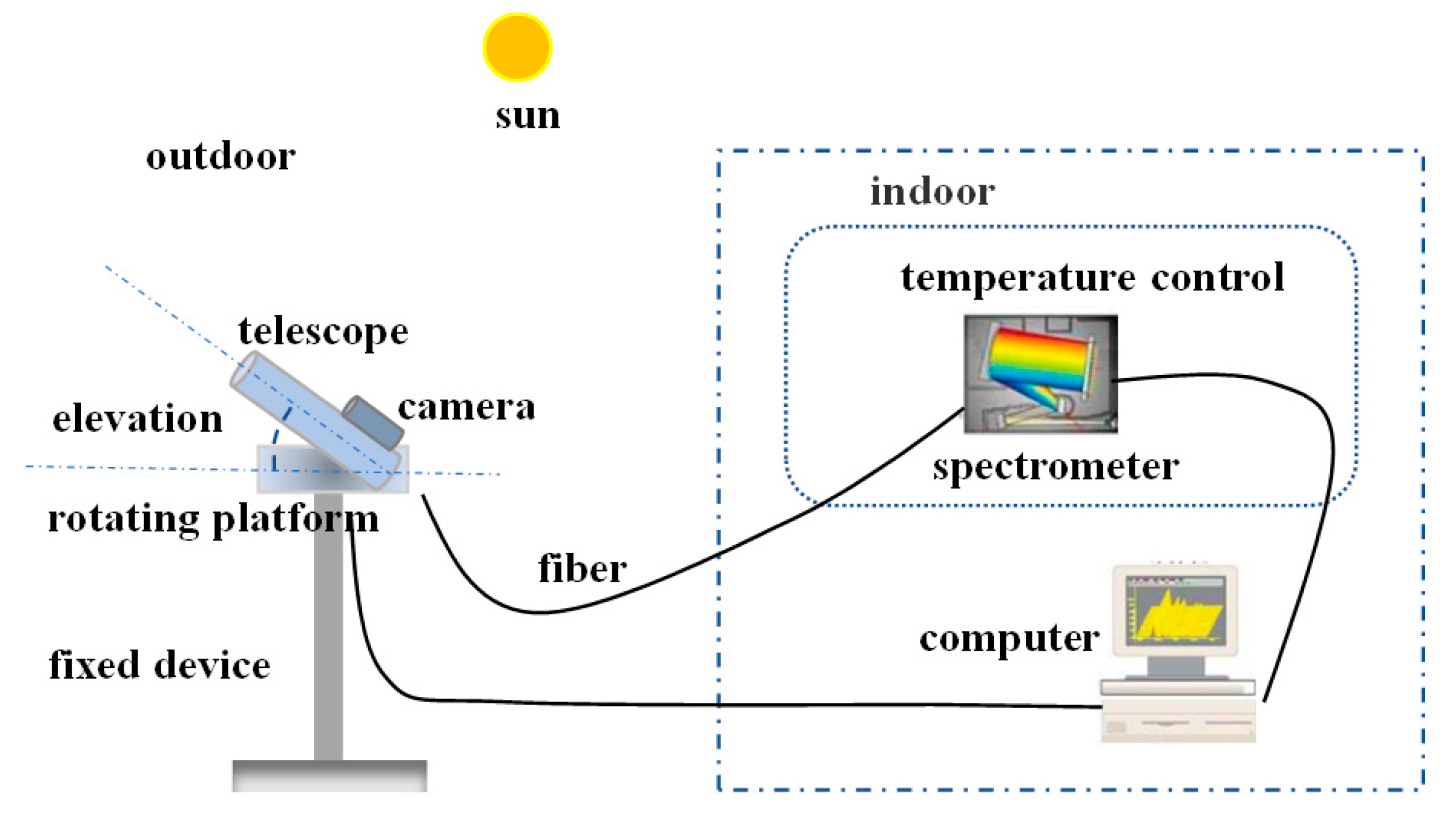
2.2. MAX-DOAS Retrieval

MAX-DOAS is a type of passive DOAS technology, theoretical basis of which is Lambert–Beer’s law [14], which is as follows:

$$I\left(\lambda \right)=I_0\left(\lambda \right)exp(-{\displaystyle \sum }_{j=1}^n{\sigma }^j\left(\lambda \right)c_j)$$

(1)

where $I\left(\lambda \right)$, $I_0\left(\lambda \right)$, ${\sigma }^j\left(\lambda \right)$, and $c_j$ are the measured spectrum after extinction in the atmosphere, the spectrum at the top of the atmosphere without extinction, the absorption cross-section and the column density of the species $j$, respectively.

The spectra were fitted with the QDOAS software, developed by the Royal Belgian Institute for Space Aeronomy, Brussels, Belgian (version 3.2, 2017) to retrieve the gas slant column density (SCD) [32]:

$$SCD={{\displaystyle \int }}^{}c\left(s\right)ds$$

(2)

where $ds$ represents the integral along the optical path. Usually, one converts the SCD to the vertical column density (VCD):

$$VCD={{\displaystyle \int }}^{}c\left(z\right)dz$$

(3)

which represents the integrated concentration (c(z)) of trace gas through the atmosphere along the vertical path. $dz$ is the vertical component of $ds$. The VCD only depends on the distribution of trace gas concentration with height, rather than the observation method and light absorption path.

The air mass factor (AMF) is often used to describe the absorption path of gases in the atmosphere, and it refers to the degree of influence of atmosphere scattering on the sunlight received by the earth’s surface [33,34,35]. AMF is defined as the ratio of the SCD to the VCD. Therefore, the VCD can be calculated by AMF and SCD:

$$VCD=\frac{\mathrm{SCD}}{\mathrm{AMF}}$$

(4)

The 90° spectra in each elevation cycle were used as the Fraunhofer reference spectrum (FRS), allowing the gas tropospheric differential slant column density (dSCD) to be retrieved. Combined with AMF, the SCD is converted into the tropospheric VCD. The tropospheric VCD can be expressed as follows [36]:

$$VCD=\frac{\Delta SCD}{\Delta AMF}=\frac{dSC{D}_{\alpha \ne 90°}-dSC{D}_{\alpha =90°}}{AM{F}_{\alpha \ne 90°}-AM{F}_{\alpha =90°}}$$

(5)

The AMF can be calculated using the atmospheric radiation transmission model (RTM). Here, we used SCIATRAN 2.2 [37] to calculate the AMF at 20° and 90° elevation angles and thereby obtained the ΔAMF ($AM{F}_{20°}-AM{F}_{90°}$) [16]. Then, the tropospheric VCD was calculated by combining the ΔAMF with the ΔSCD ($dSC{D}_{20°}-dSC{D}_{90°}$).

2.3. Precipitable Water

PW is defined as [1]

$$PW={{\displaystyle \int }}_0^{z_t}c\left(z\right)dz$$

(6)

where $z_t$ represents the height of the tropopause, and PW represents the integrated concentration of water vapor (c(z)) along the vertical path, corresponding to the total amount of water vapor contained in the air column.

It can be seen that the PW and tropospheric VCD have the same definition and physical meaning, so their numeric values are equal. The unit of VCD is generally expressed in molecules/m², which can be converted into the same unit as that of PW—namely, kg/m². In addition, the unit of PW can also be expressed in mm [1].

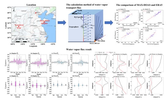
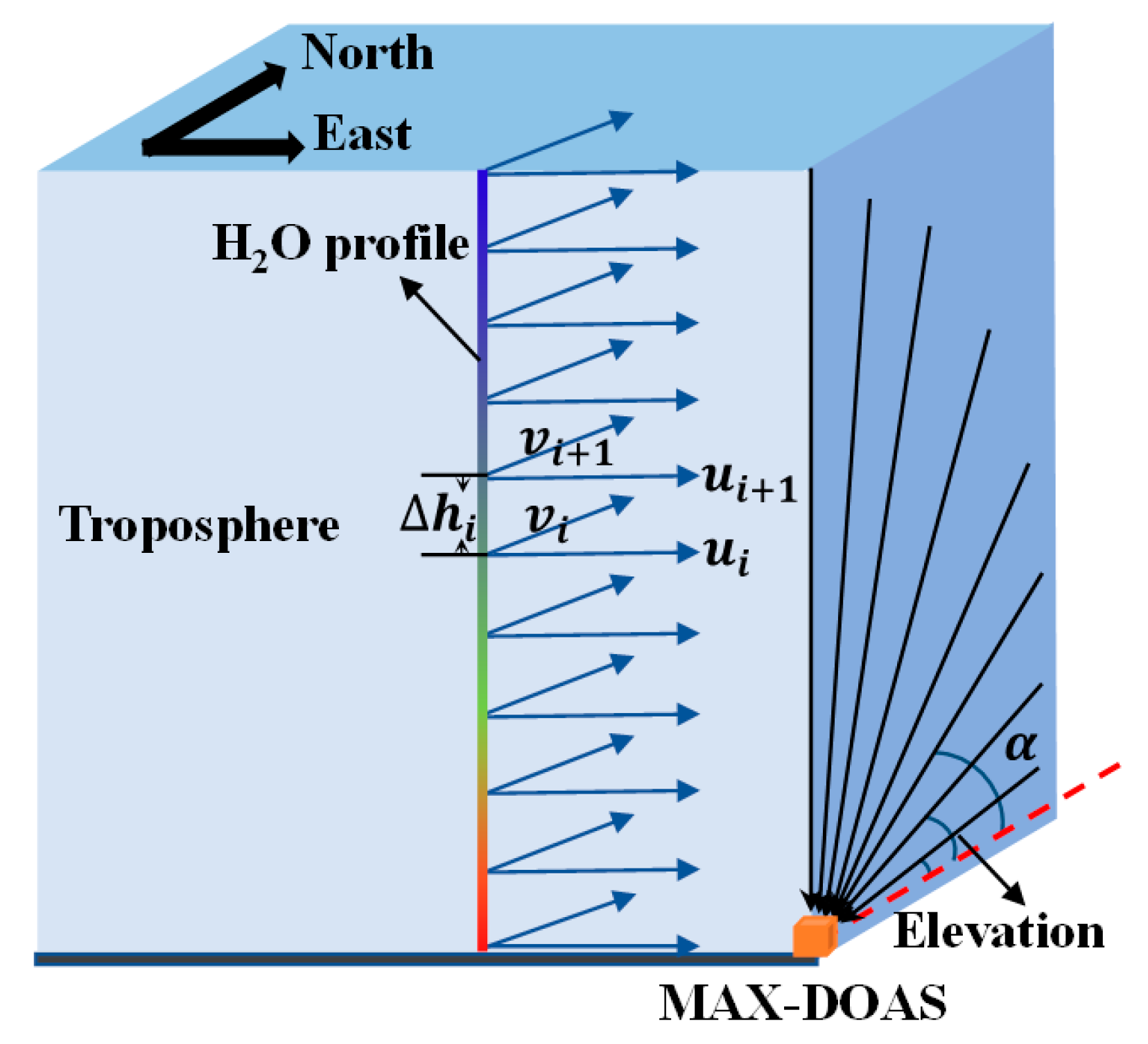
2.4. Water Vapor Flux

WVF can be decomposed into the two components of meridional and zonal transportation, and its magnitude depends on the wind field and water vapor concentration profile.

The PriAM algorithm developed by the AIOFM of the Chinese Academy of Sciences and the Max Planck Institute of Chemistry (MPIC), Germany was used for the water vapor concentration profile retrieval in this study [16]. The universality of the PriAM algorithm has been demonstrated in many comparative observation experiments [17,18,19,20]. The PriAM algorithm is mainly used to solve the nonlinear retrieval problem of iterative equations based on the optimal estimation (OE) method. RTM is used as the forward model function $F$ to simulate the measurement vector $y$ (it represents the dSCD from each elevation angle, with M elements) on the basis of the atmospheric state vector $x$ (it represents the gas concentration at each height, that is, the gas profile, with N elements) obtained from the retrieval. By adjusting the input parameters of the model (prior gas profile, etc.), PriAM iterates many times until the optimal result is obtained. The iterative equation is expressed as

$$x_{i+1}=x_i+{\left[K_i^{\mathrm{T}}{S}_{\epsilon }^{-1}{K}_i+\left(1+{\gamma }_i\right)S_a^{-1}\right]}^{-1}\left\{K_i^{\mathrm{T}}{S}_{\epsilon }^{-1}\left[y-F\left(x_i\right)\right]-S_a^{-1}\left[x_i-x_a\right]\right\}$$

(7)

where $x_{i+1}$ and $x_i$ are the current and previous state vectors, respectively. $S_{\epsilon }$ is the measurement error covariance matrix (M × M), and $K_i$ is the weight function matrix (in which each element is the partial derivative of a measurement vector component over a state vector). ${\gamma }_i$ is a correction coefficient to update each iteration to optimize the retrieval. It can be set to 1 at first and then modified according to the iteration situation. $S_a$ is the prior error covariance matrix (N × N). In this study, the prior water vapor profile used the monthly average of local sounding data, and the prior iteration number was 20.

Because the aerosol state affects the transmission path of light in the atmosphere, which will affect the retrieval of the vertical distribution of trace gases, the retrieval process needs to be performed in two steps. First, it is necessary to retrieve the vertical profile of the aerosol extinction coefficient (AEC) from the O₄ dSCD based on the OE method. Then, the water vapor vertical profile and tropospheric (about 10–12 km) water vapor VCD are retrieved from the AEC profile. Because MAX-DOAS is not sensitive to the upper atmosphere, this study only retrieved the water vapor profile at around 0.05–4 km above the surface.

The hourly wind profiles ($u_i$ and $v_i$) for the study were downloaded from the ERA5 reanalysis datasets (https://cds.climate.copernicus.eu (accessed on 3 August 2020)). $u_i$ is the zonal wind speed (m/s), and $v_i$ is the meridional wind speed (m/s). ERA5 is ECMWF’s latest climate reanalysis product and uses advanced modeling and data assimilation systems to combine vast amounts of historical observations into global estimates, thereby providing hourly data on various atmospheric, surface, and ocean parameters, as well as the relevant uncertainties. The horizontal distance resolution of ECMWF ERA5 is 0.25° × 0.25°, and the vertical altitude is divided into 37 layers according to atmospheric pressure from 1000 to 1 hPa (

Table 2. European Centre for Medium-Range Weather Forecasts (ECMWF) ERA5 pressure levels and MAX-DOAS levels.

ECMWF ERA5 Pressure Levels (hPa)								MAX-DOAS Levels (km)
1000	975	950	925	900	875	850	825	0.05	0.2	0.4	0.6	0.8
800	775	750	700	650	600	550	500	1	1.2	1.4	1.6	1.8
450	400	350	300	250	225	200	175	2	2.2	2.4	2.6	2.8
150	125	100	70	50	30	20	10	3	3.2	3.4	3.6	3.8
7	5	3	2	1				4

). The atmospheric pressure was converted to altitude in our study using the barometric altitude formula [38].

The time resolution of the water vapor profile obtained by MAX-DOAS is usually 3 to 5 min. All the water vapor profiles within ±0.5 h of the corresponding times in the wind profiles were coupled with the same wind profile. For example, the water vapor profile from 7:31 to 8:30 used the wind profile at 8:00. The water vapor profile was divided into 21 layers; the lowest was 0.05 km, and the highest was 4 km (Table 2). The wind profile was interpolated to each layer height of the water vapor profile, and the exponential interpolation function was selected according to the curve fitting effect of the wind profile (see Section 2.6). According to the water vapor transport flux calculation formula, the zonal water vapor transport flux ($Q_{\lambda ,i,t}$) and meridional water vapor transport flux ($Q_{\phi ,i,t}$) of the i-th layer at time t were as follows:

$$Q_{\lambda ,i,t}={\left(x_i{u}_i\right)}_t,Q_{\phi ,i,t}={\left(x_i{v}_i\right)}_t$$

(8)

where $x_i$ is the water vapor concentration of the i-th layer (kg/m³); $\lambda$ and $\phi$ represent the zonal and the meridional, respectively. The unit of water vapor transport flux in the i-th layer is kg/m²/s.

In addition, there were random errors in the measurement of the water vapor profiles; we reduced these errors via statistical averaging. The average value of the water vapor profile from t − Δt to t + Δt (Δt represents the time range of the statistics) was used as the water vapor profile at time t. The corrected zonal water vapor transport flux (${\overline{Q}}_{\lambda ,i,t}$) and meridional water vapor transport flux (${\overline{Q}}_{\phi ,i,t}$) at time t are calculated as follows:

$${\overline{Q}}_{\lambda ,i,t}=((\frac{1}{N}{{\displaystyle \sum }}_j{x}_{i,j})u_i{)}_t,{\overline{Q}}_{\phi ,i,t}=((\frac{1}{N}{{\displaystyle \sum }}_j{x}_{i,j})v_i{)}_t$$

(9)

where j represents the j-th time in the time period from t − Δt to t + Δt, and N represents the number of water vapor profiles in this time period. In our study, Δt is 15 min.

The zonal and the meridional water vapor transport flux of each layer at time t were superposed and summed to obtain the vertically integrated zonal water vapor transport flux (${\overline{Q}}_{\lambda ,t}$) and vertically integrated meridional water vapor transport flux (${\overline{Q}}_{\phi ,t}$), respectively:

$$\begin{gathered} {\overline{Q}}_{\lambda ,t}={{\displaystyle \sum }}_i(\mathsf{\Delta }{h}_i·{\overline{Q}}_{\lambda ,i,t})={{\displaystyle \sum }}_i(\mathsf{\Delta }{h}_i·(\frac{1}{N}{{\displaystyle \sum }}_j{x}_{i,j})u_i{)}_t, \\ {\overline{Q}}_{\phi ,t}={\displaystyle \sum }_i(\mathsf{\Delta }{h}_i·{\overline{Q}}_{\phi ,i,t})={\displaystyle \sum }_i(\mathsf{\Delta }{h}_i·(\frac{1}{N}{\displaystyle \sum }_j{x}_{i,j})v_i{)}_t \end{gathered}$$

(10)

where $\Delta h_i$ is the height resolution of the i-th layer of the water vapor profile.

Due to the limitation of MAX-DOAS’s detection height, the water vapor transport flux analysis here focuses on the vertically integrated transport flux up to 4 km above the ground. Because 75–80% of the water vapor is concentrated below 4 km, this flux captures the dominant transport of water vapor in the lower troposphere. The unit of vertically integrated water vapor transport flux is kg/m/s. Figure 3 presents the principle of the water vapor transport flux estimation method used by MAX-DOAS.

Water vapor transport is the main factor leading to precipitation. Therefore, using MAX-DOAS to calculate the water vapor transport flux at different altitudes is of great significance for the study of precipitation formation.

2.5. Precipitable Water and Water Vapor Flux Error Sources

When a new calculation method of PW and WVF is presented, it is very necessary to consider its error.

2.5.1. Precipitable Water Error Sources

The uncertainty of using the MAX-DOAS instrument to retrieve PW (water vapor VCD) was mainly caused due to SCD fitting errors and AMF errors. Generally, the water vapor SCD fitting error was ≤3% [21,22,23,24], and the error we fitted via QDOAS 3.2 was also ≤3%. The AMF error was caused by the uncertainty of the input parameters (solar zenith angle, relative azimuth angle, surface albedo, water vapor profile, etc.) in the RTM, and typically, average error ranged from 8% to 24% [21,22,23,24]. We estimated the contribution of each input parameter to the overall AMF uncertainty via SCIANTRAN 2.2 and found that the average error of AMF was less than 15%. Therefore, the total error of PW was less than 15%.

2.5.2. Water Vapor Flux Error Sources

The uncertainty of the WVF was mainly caused by DOAS fitting errors, water vapor profile retrieval errors, and wind field and height uncertainty. We analyzed these errors based on different sources.

a. The DOAS fitting error was ≤3% (see Section 2.5.1).

b. Because the water vapor profile was retrieved by PriAM, its errors could be attributed to a smoothing error ($S_s$), input parameter error ($S_m$), or residual error ($S_r$) [16]. The total retrieval error of the water vapor profile is taken as the root mean square of these three errors. The calculation equations for these three errors are:

$$S_s={\left(K^T{S}_{\epsilon }^{-1}K+S_a^{-1}\right)}^{-1}{S}_a{\left(K^T{S}_{\epsilon }^{-1}K+S_a^{-1}\right)}^{-1}$$

(11)

$$S_m={\left(K^T{S}_{\epsilon }^{-1}K+S_a^{-1}\right)}^{-1}{K}^T{S}_{\epsilon }^{-1}K{\left(K^T{S}_{\epsilon }^{-1}K+S_a^{-1}\right)}^{-1}$$

(12)

$$S_r={\left(K^T{S}_c^{-1}K+S_a^{-1}\right)}^{-1}{K}^T{S}_c^{-1}K{\left(K^T{S}_c^{-1}K+S_a^{-1}\right)}^{-1}$$

(13)

where $S_c$ is the covariance matrix of the difference between the simulated value and the measured value. The total error of the water vapor mixing ratio retrieved from PriAM was found to be less than 20% in this study.

c. The uncertainty of the wind field includes the uncertainty of the wind speed and wind direction. Because the ECMWF ERA5 wind profile was used to couple the water vapor concentration profile, the main source of wind field uncertainty was from the ERA5 wind profile. A previous study showed that the statistical deviation between the ERA5 wind profile and the near-surface measurement data was as follows: the near-surface wind speed uncertainty was ±1 m/s, and the wind direction uncertainty was ± (20° to 60°) [39]. We also compared the ERA5 wind profile with the near-surface measurement data, and the results showed that the deviation of wind speed was ±1.1 m/s, while the wind direction was ±(0° to 63°).

d. The uncertainty of height is mainly because the water vapor concentration was considered to be uniform within 200 m in the flux calculation formula. We assumed that the water vapor concentration would decrease exponentially (ignoring cyclogenesis and deep convection). The difference between the constant water vapor concentration and the exponentially changing water vapor concentration within 200 m was the uncertainty introduced by the height change. In this study, the error evaluation result was about 6%.

The total error of WVF is represented by the root mean square of the above four typical errors. Generally, the average method reduced the random error caused by the DOAS fitting, and the main error sources for the WVF estimation by MAX-DOAS were profile retrieval errors and wind field and height uncertainty.

The total error of WVF is expressed as

$$\Delta Q=\sqrt{\Delta Q_{Fitting}^2+\Delta Q_{profile}^2+\Delta Q_{\underset{W}{\to }}^2+\Delta Q_{height}^2}$$

(14)

where $\Delta Q_{Fitting}$, $\Delta Q_{profile}$, $\Delta Q_{\underset{W}{\to }}$, and $\Delta Q_{height}$ represent the DOAS fitting error, water vapor profile retrieval error, wind field error, and height error, respectively. The total errors totaled less than 36% in the most exceptional situation.

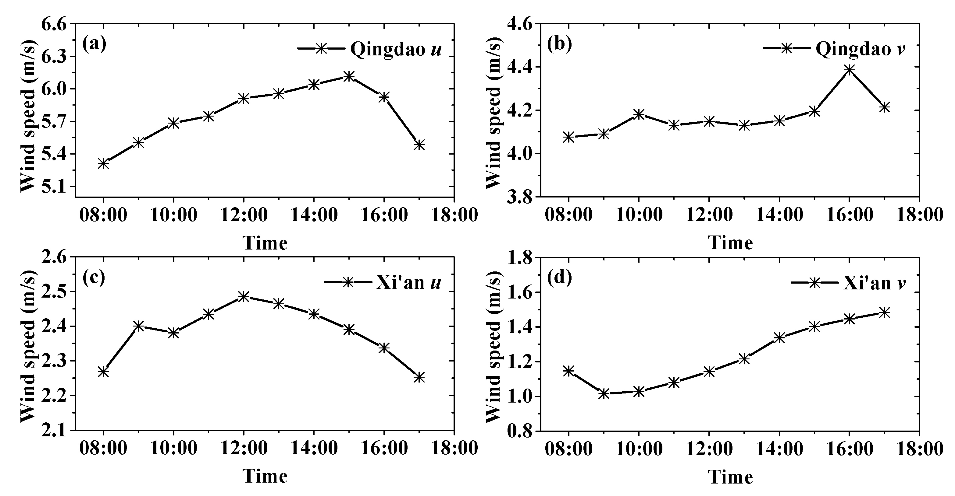
2.6. Selection of the Wind Profile Interpolation Function

In this study, MAX-DOAS observations in Qingdao and Xi’an were carried out from 1 June 2019 to 31 May 2020; then, the water vapor zonal and meridional transport flux were calculated. The number of effective days at Qingdao was 282 days, and that at Xi’an was 276 days, excluding rainy weather. The measurement dates were divided into four seasons: March, April, and May were spring; June, July, and August were summer; September, October, and November were autumn; and December, January, and February were winter.

To interpolate the wind profile to the height of the water vapor concentration, we downloaded the wind profile data of the two cities in the observation period (one year) from the ECMWF ERA5 reanalysis datasets. Because MAX-DOAS only measures during the daytime, the wind profiles for 8:00, 9:00, 10:00, 11:00, 12:00, 13:00, 14:00, 15:00, 16:00, and 17:00 (UTC+8) were selected. Firstly, we averaged the wind profiles for the 4 seasons. Then, we fitted the curve with exponential types (Figure 4). According to the $u$ and $v$ wind fitting effects of Qingdao and Xi’an (R² ≥ 0.9), it was advisable to use an exponential function for the interpolation computation.

3. Results and Discussion

3.1. Comparison of MAX-DOAS and ERA5 Reanalysis Datasets

To verify the accuracy of the PW and WVF from the MAX-DOAS measurements, the measurement data (PW and the zonal and meridional water vapor transport flux) for Qingdao and Xi’an from September to October 2019 were compared with the ECMWF ERA5 reanalysis datasets.

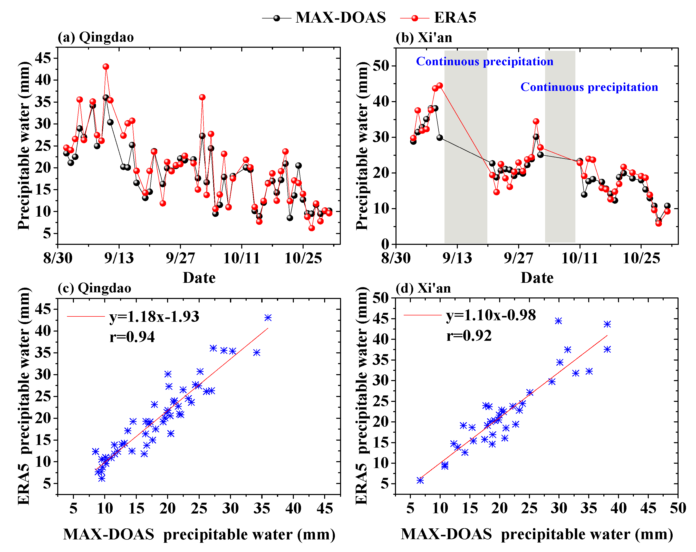
3.1.1. Precipitable Water Comparison

The comparison results of the PW in the two cities are shown in Figure 5. The shaded area in the figure indicates continuous precipitation weather and that the measurement was invalid. Here, the PW correlation coefficients (r) between the MAX-DOAS measurements and the ERA5 reanalysis datasets of Qingdao and Xi’an are r = 0.94 and r = 0.92, respectively. In previous studies, PW (water vapor VCD) was also compared with a variety of other datasets. For example, the water vapor VCD from MAX-DOAS measurements in Mainz, Germany was compared with the Aerosol Robotic Network (AERONET), satellite observations, and the surface; good agreements were found between all measurements [21]. The water vapor VCD according to MAX-DOAS measurements in Beijing, China was likewise compared with AERONET (r = 0.92) [27]. The high correlation ensured the accuracy of PW using MAX-DOAS measurements.

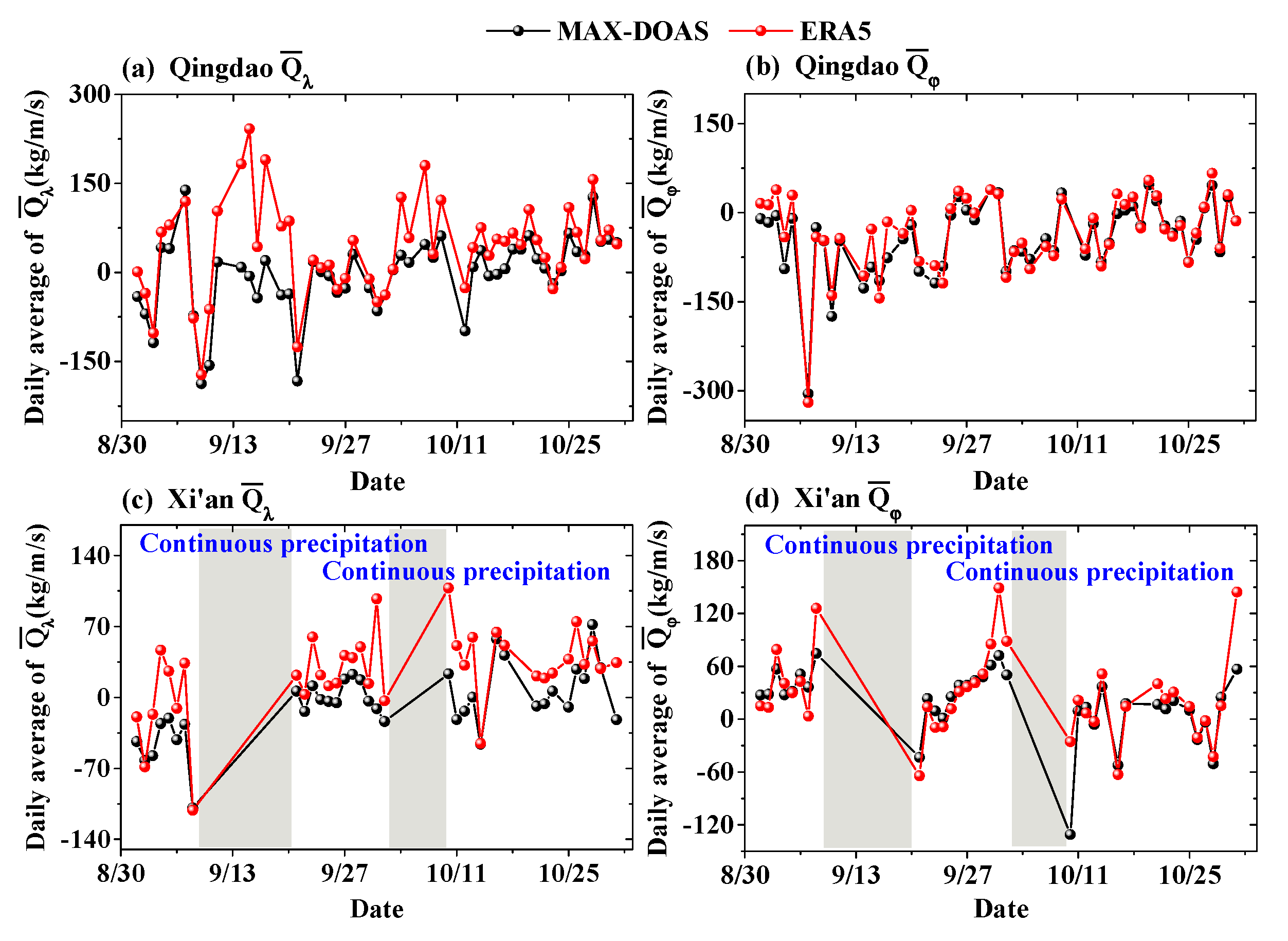
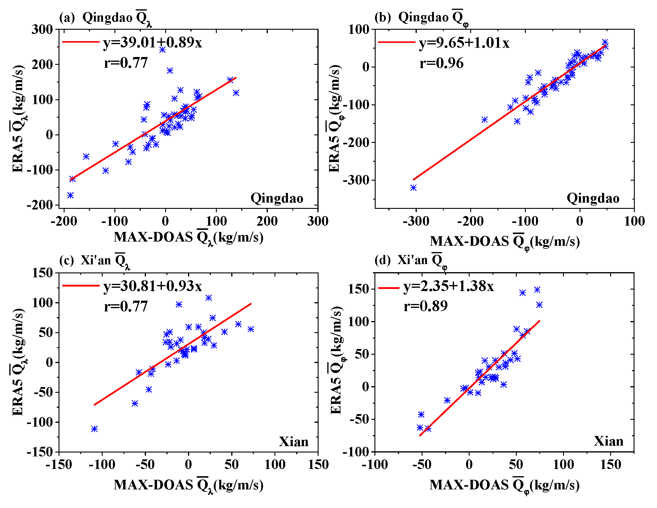
3.1.2. Water Vapor Flux Comparison

We compared the WVFs from the MAX-DOAS observations with the ERA5 WVFs (Figure 6). The correlation coefficients of ${\overline{Q}}_{\lambda }$ between the two datasets were both 0.77 in Qingdao and Xi’an (Figure 7a,c). The correlation coefficients of ${\overline{Q}}_{\phi }$ between the two datasets were 0.96 in Qingdao (Figure 7b) and 0.89 in Xi’an (Figure 7d). The zonal flux comparison results were slightly worse than the meridional results. The water vapor transport flux derived from MAX-DOAS only superimposed the WVF from 0 to 4 km, and ERA5 is tropospheric, which leads to a certain difference between the two datasets. The comparison results show that the new method of calculating the WVFs from the MAX-DOAS observations is credible.

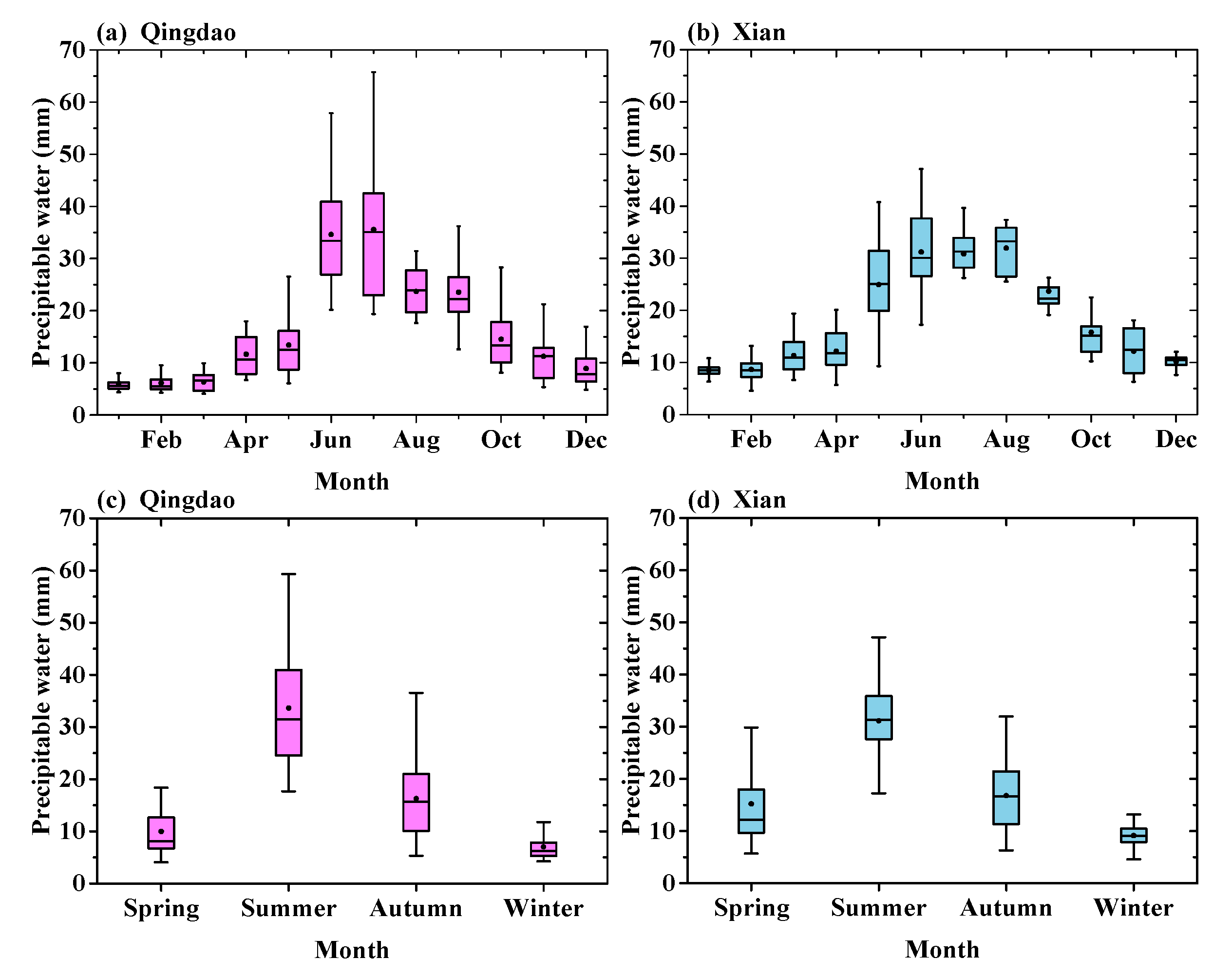
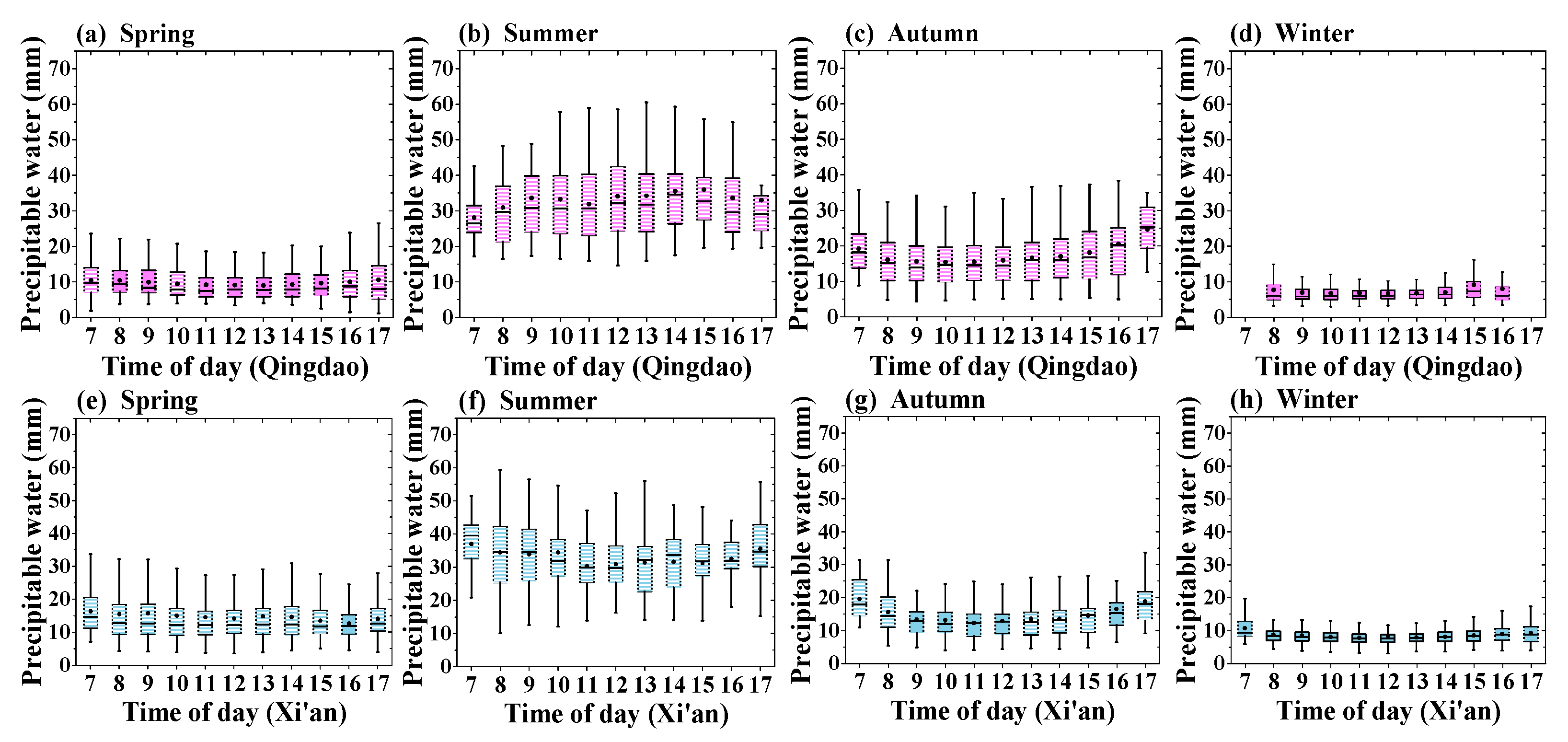
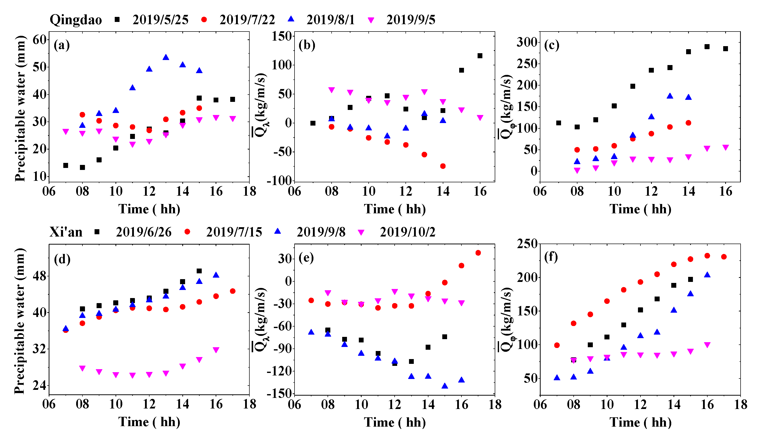
3.2. Precipitable Water Variations in Qingdao and Xi’an

To investigate the similarities and differences of the PW in the two cities, the monthly and seasonal PW values from MAX-DOAS instruments were calculated (Figure 8). The seasonal variation of the PW was similar in Qingdao and Xi’an, with the maxima in summer and minima in winter (see Figure 8c,d). The median PW ranged from 5.54 (February) to 35.07 mm (August) in Qingdao and from 8.48 (January) to 33.25 mm (August) in Xi’an (see Figure 8a,b). The median characterizes the general situation of the PW. As shown in Figure 8, there was no significant seasonal difference in the median PW, although the two cities are geographically disparate.

The diurnal variations of the PW in the two cities (Figure 9) exhibited large variability in all seasons. Three seasons (excluding summer (see Figure 9b) in Qingdao (Figure 9a,c,d) and four seasons in Xi’an (Figure 9e–h) all show that the median PW values were higher in the morning and in the afternoon than at noon. A higher PW indicates an increase in the water vapor VCD. Therefore, this diurnal variation was mainly due to the low temperature and high humidity in the morning and in the afternoon. In addition, the diurnal variation of PW in summer was different from that during other seasons in Qingdao, which was related to the geographical location of Qingdao. In addition, a previous study showed that precipitation increased to extreme levels when the temperature reached 25° in Qingdao city [40]. Therefore, at noon in the summer, as the temperature became higher than 25°, the PW also increased. The median PW during the afternoon in Qingdao was higher than that in the morning, which agrees with a previous study [1]. This also shows the feasibility and advantage of using MAX-DOAS to measure PW.

The diurnal variations in PW showed regional differences between the two cities, but the variation ranges in other seasons were relatively small, except during the summer.

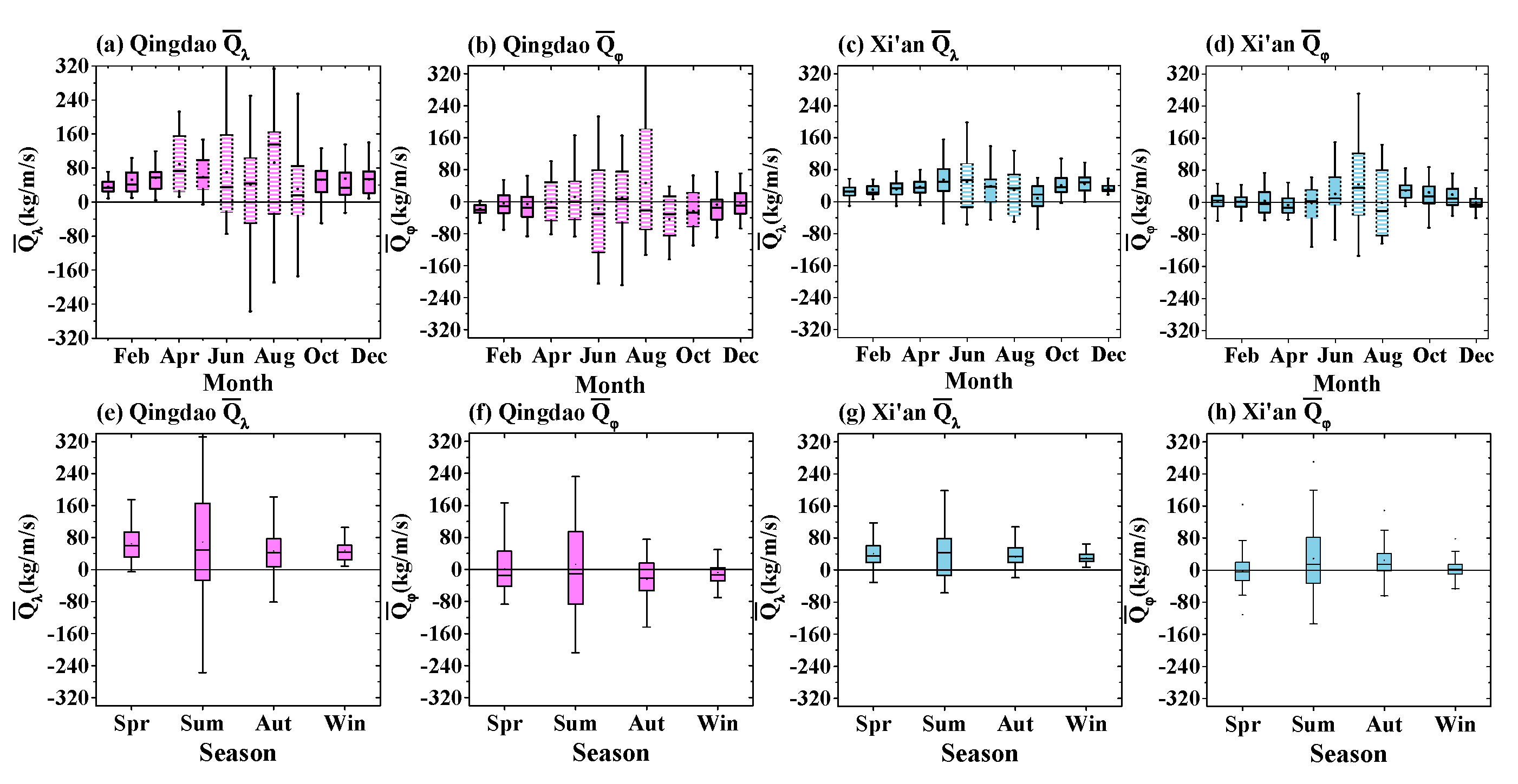
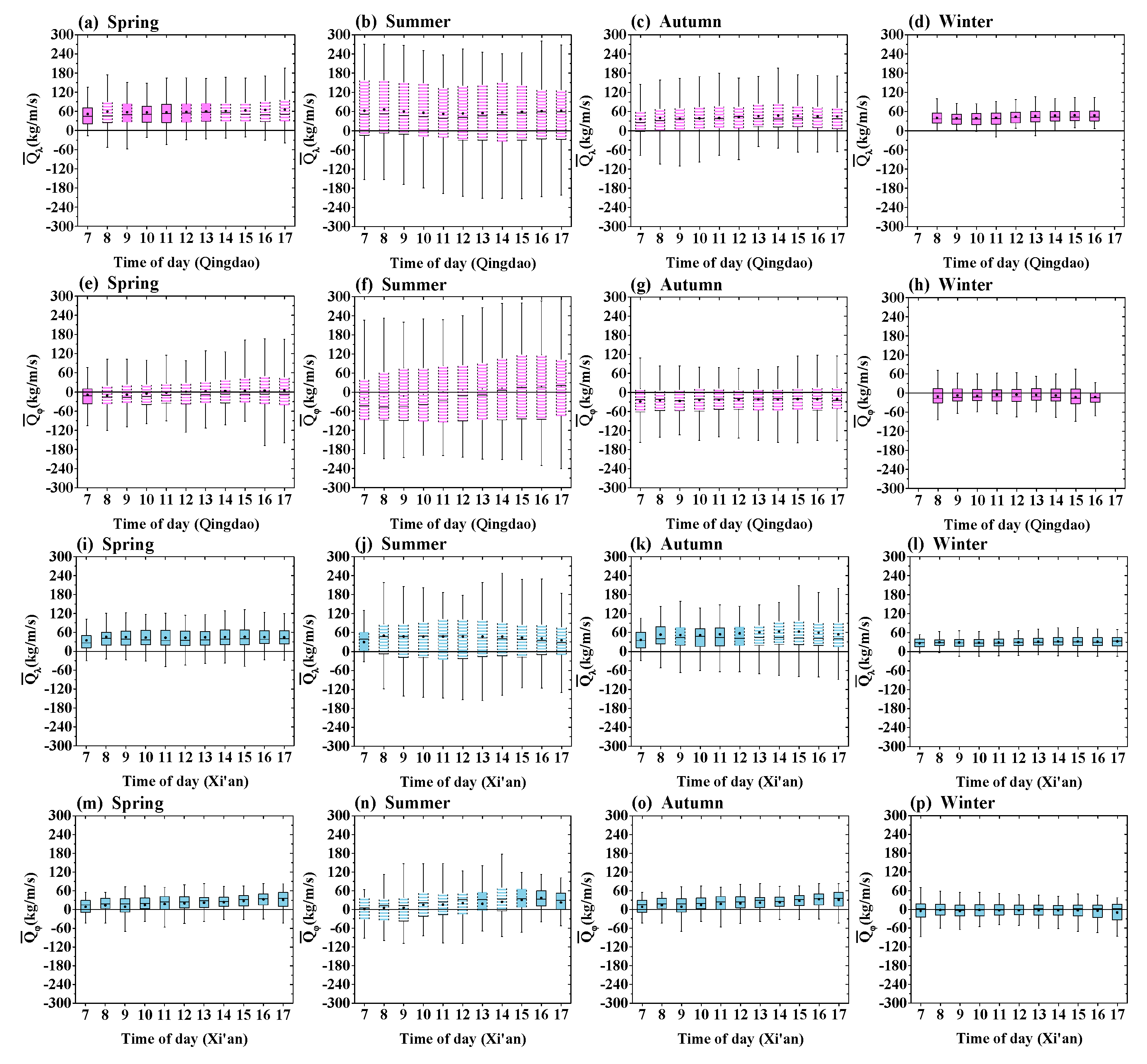
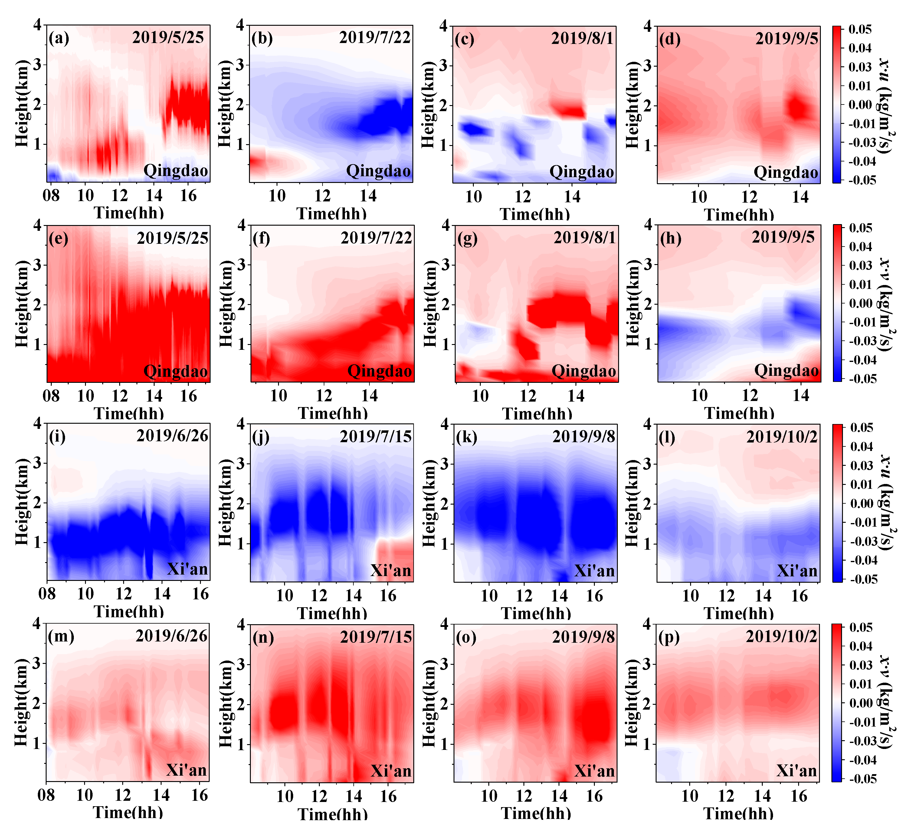
3.3. Water Vapor Flux Variations in Qingdao and Xi’an

WVF is important for the study of water cycles. To further understand the water cycles of the inland (Xi’an) and coastal (Qingdao) cities in China, we analyzed the seasonal and diurnal variations of the water vapor transport fluxes in the two cities. Figure 10 shows the monthly and seasonal variation of the vertically integrated WVFs. The seasonal variations in the WVFs were similar to those of the PW, with the maxima in the summer months and the minima in the winter months.

The median of the zonal WVFs in Qingdao was the largest in August (135.65 kg/m/s) and the smallest in September (16.42 kg/m/s). The median of the zonal WVFs in Xi’an was the largest in June (54.60 kg/m/s), and the smallest was also in September (18.10 kg/m/s). The zonal water vapor transport fluxes of the two cities were negative (transport from east to west), except for a few days in June, July, August, and September that featured high temperatures. This indicates that for both the inland city (Xi’an) and coastal city (Qingdao), water vapor was mainly transported from west to east. While the two cities are located in mid-latitude regions, where westerly wind dominates at high levels, the above results are also related to seasonal variations in the water vapor concentration and not solely on variations in the zonal wind [1].

The median of the meridional WVFs in Qingdao was the largest in June at −31.10 kg/m/s and the smallest in May at −0.32 kg/m/s, while the median in Xi’an was the largest in July at 36.46 kg/m/s and the smallest in February at 2.23 kg/m/s. Negative indicates transport from north to south, while positive indicates transport from south to north. The meridional WVF medians in Qingdao were positive in May and July but were negative for the other months. Therefore, the meridional water vapor mainly featured southward transport in Qingdao. The medians of the meridional WVFs in Xi’an were negative in March, April, August, and December but were positive for the other months. Therefore, the meridional water vapor mainly indicated northward transport in Xi’an. Due to the large difference in the longitude (12.62°) and geographic situation between the two cities, there was a greater difference between the two cities in the meridional water vapor transport flux than in the zonal flux. Because Qingdao is located along the coast, and the wind speed in coastal cities is higher than that in inland cities, the water vapor transport flux of Qingdao is generally greater than that of Xi’an.

Figure 11 shows the diurnal variations of the vertically integrated WVFs in Qingdao and Xi’an in different seasons. The water vapor transport fluxes of the two cities in the afternoon were larger than those in the morning. This may be related to the wind speed, so we plotted the diurnal variations curve of the wind speed during the observation period (Figure 12). Figure 12 shows that the wind speed in the two cities tended to increase in the afternoon, which caused the WVFs to increase in the afternoon. In addition, as shown in Figure 12, the wind speed in Qingdao was significantly higher than that of Xi’an.

Overall, the range of diurnal variation in Xi’an for each season was smaller than that of Qingdao. Because the seasonal and diurnal variations of PW (water vapor VCD) in the two cities are not significantly different (Figure 8 and Figure 9), the water vapor transport flux differences between the two cities were mainly caused by differences in wind direction and wind speed.

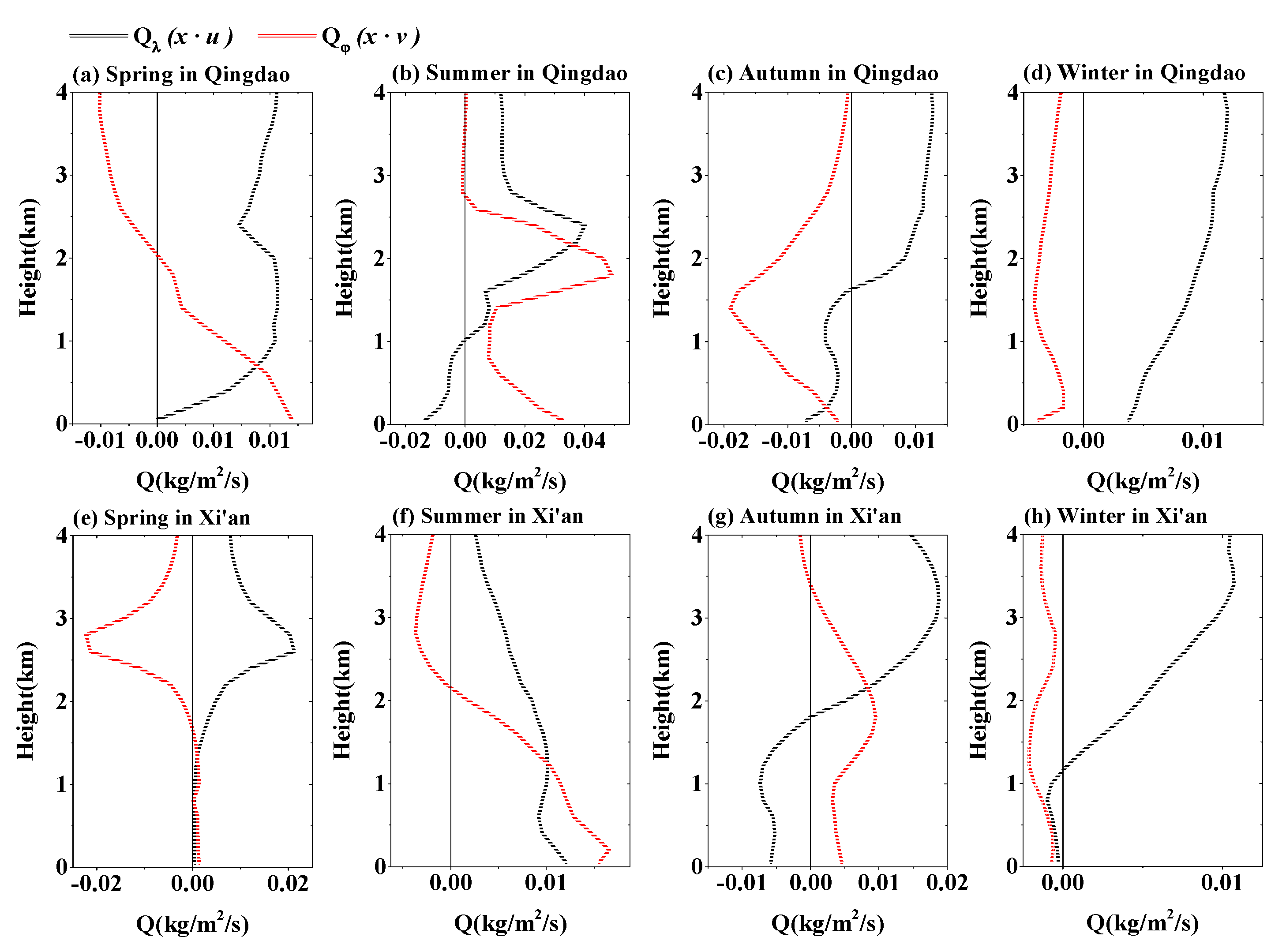
3.4. Water Vapor Flux Profile in Qingdao and Xi’an

The zonal and meridional WVF profiles based on MAX-DOAS observations were averaged for each season (Figure 13).

In Qingdao, the zonal and meridional WVFs were the largest in summer; the zonal WVF reached its maximum of 4.02 × 10⁻² kg/m²/s at 2.4 km, and the meridional WVF reached its maximum of 4.92 × 10⁻² kg/m²/s at 1.8 km (Figure 13b). However, the high levels of water vapor transport in summer and autumn were more striking. The WVF transmitting belts in summer and autumn were distributed around 2 and 1.4 km, respectively, and featured similar shapes in the zonal and meridional directions (Figure 13b,c). In this study, the WVF transmitting belt was defined as a high-value area above the surface—that is, the flux in this area is higher than the flux at the upper and lower adjacent heights.

In Xi’an, the water vapor transport fluxes were the largest in spring; the maximum zonal WVF was 2.13 × 10⁻² kg/m²/s at 2.6 km, and the maximum meridional WVF was −2.23 × 10⁻² kg/m²/s at 2.8 km. The WVF transmitting belt was more obvious in spring and autumn, and the zonal WVF featured a transmitting belt at around 2.6 and 1.0 km, while the meridional WVF featured a transmitting belt at around 2.8 and 1.6 km (Figure 13e,g).

In addition, due to the effects of atmospheric circulation and turbulence, the wind direction near the ground at high altitudes may be opposite, resulting in different transport directions. For example, the direction of the meridional water vapor transport flux reversed at 2 km in Qingdao during spring (Figure 13a), and the direction of the zonal water vapor transport flux reversed at 1.8 km during autumn in Xi’an (Figure 13g). In Xi’an, the WVFs at high altitudes (about 2–3 km) were larger than those near the ground, except for the summer, which can be attributed to a combination of the water vapor concentration and the wind profile.

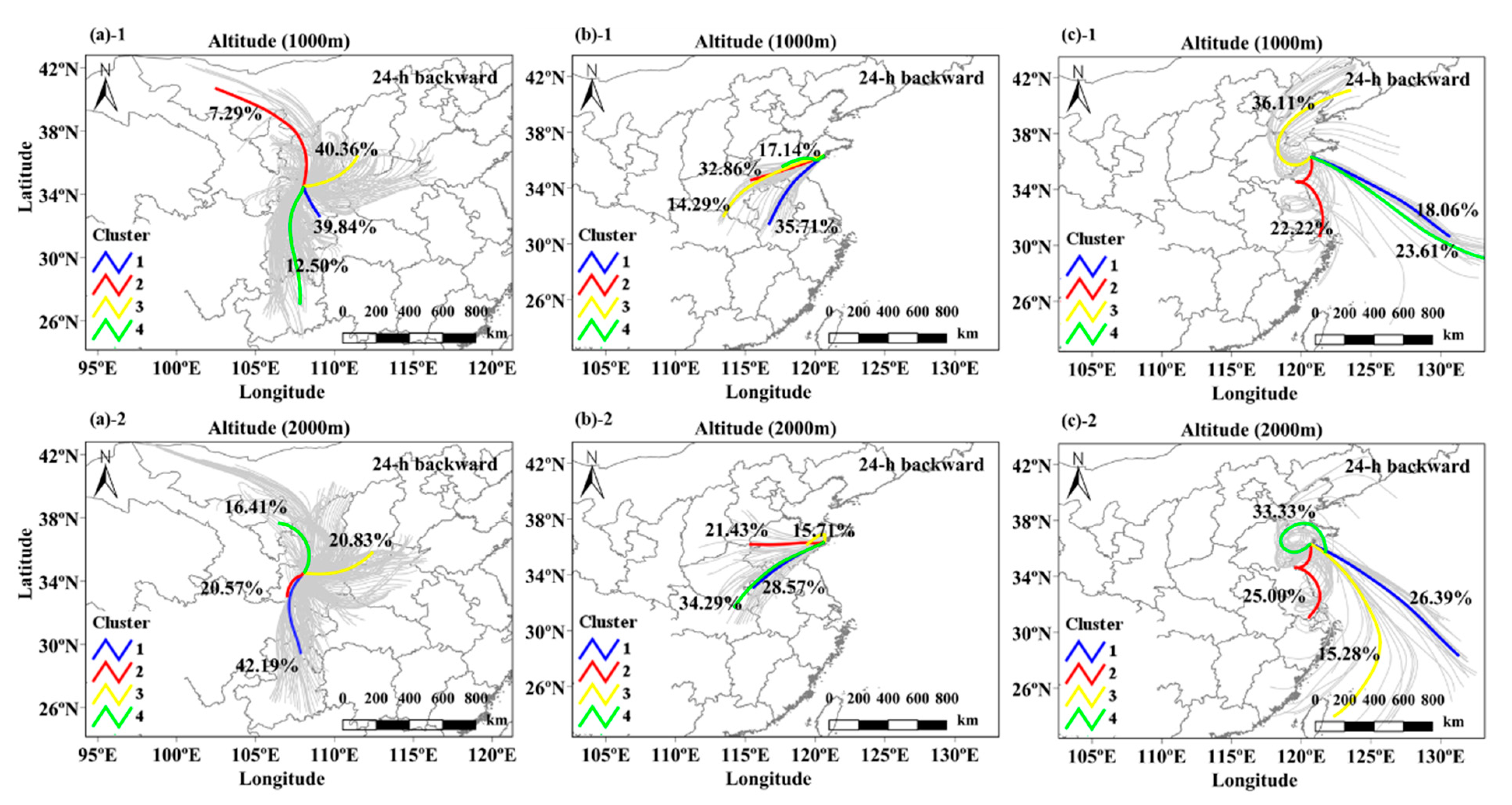
3.5. Water Vapor Transport before Precipitation

The occurrence of precipitation is closely related to the transport of water vapor [41,42]. The flux profile of the day before precipitation was plotted according to local weather data. Four days of measurement data from the two cities were selected as the cases to study (Figure 14). Figure 14a–h indicates that the WVF transmitting belt before precipitation moved from a low level of about 0.5 km to a high level of about 2 km in Qingdao. In Xi’an, the WVF transmitting belt before precipitation also featured a small upward trend and finally moved to around 1 and 1.8 km (Figure 14i–p). These results indicate that the WVF transmitting belt moved from near ground to a high level before precipitation, and the flux reached its maximum at around 2 km. This also indirectly reflected the bottom-up transport process of water vapor before precipitation, which accumulated at about 2 km. When it reached a certain amount, the water vapor promoted precipitation.

All four water vapor transport fluxes in Xi’an before precipitation show that the zonal flux was negative (westward transport), while the meridional flux was positive (northward transport). This relates to the circulation of the atmosphere and the transport of water vapor, and the humid air in the southeast is likely to cause considerable water vapor to accumulate in the sky above Xi’an, leading to precipitation.

Figure 15 shows that the PW and meridional vertically integrated water vapor transport fluxes of the two cities experienced an increasing trend on the day before the precipitation, which is similar to the results of previous reports [43]. Moreover, the meridional vertically integrated water vapor transport fluxes of the two cities were positive before precipitation, which indicates that the transport of water vapor via southerly wind provides favorable conditions for precipitation in the two cities.

The long-term observation of water vapor using MAX-DOAS, the abnormal changes in WVF, and PW serve as an important reference for precipitation forecasting.

The occurrence of continuous precipitation and torrential rain can cause disasters and have a huge impact on human production and life [44,45]. Their occurrence of these factors is closely related to water vapor transport and accumulation. To further analyze the source and transport of water vapor during the continuous precipitation and torrential rain in Qingdao and Xi’an, we selected the continuous precipitation (precipitation days ≥ 3 days) and torrential rain (daily precipitation: >50 mm) weather in the two cities during the observation period based on meteorological data (http://data.cma.cn/ (access on 10 September 2020)). The Hybrid Single-Particle Lagrangian Integrated Trajectory (HYSPLIT) model was used for cluster analysis of the backward trajectory of the air mass during continuous precipitation and torrential rain. Torrential rain occurred in Qingdao from 10 to 11 August 2019, preceded by a continuous precipitation period from 29 to 31 July 2019. There was no torrential rain in Xi’an during the measurement period, and there were three continuous precipitation periods (16–18 July 2019, 9–18 September 2019, and 3–5 October 2019). According to the transport height of the water vapor in Figure 14, heights of 1 and 2 km were used for the cluster analysis of backward trajectories (Figure 16). The 24 h air mass backward trajectories were divided into four clusters in this study.

Figure 16a indicates that the water vapor mainly came from the southeast air masses during the continuous precipitation period in Xi’an. The air masses from the southeast at heights of 1 and 2 km accounted for 93% and 84%, respectively. Figure 16b shows that during the continuous precipitation period in Qingdao, water vapor mainly came from the western (inland) air masses. During the torrential rain period in Qingdao (Figure 16c), the air masses mainly came from the ocean. The air masses from the ocean at heights of 1 and 2 km accounted for 78% and 75%, respectively. In addition, the wind speed was relatively high and accompanied by a high-altitude vortex and southeast jet movement (Figure 16c), which also led to the occurrence of torrential rain.

4. Conclusions

In our study, the ECMWF ERA5 wind profile was used to calculate the MAX-DOAS WVFs. Then, we compared the WVFs with the ECMWF ERA5 WVFs and found good agreement. However, the good agreements of the WVF comparison results only indicated the correctness of the water vapor profile based on MAX-DOAS measurements and the calculation method for the WVFs. The accuracy of the WVF results could not be proven directly because there is a large deviation between the ECMWF wind profile and the actual wind profile near the ground [39,46], which, furthermore, caused large errors in the WVFs in the study (as discussed in Section 2.5.2). A measured wind profile would greatly improve the WVF analysis results in our study. Using MAX-DOAS and wind radar to perform these measurements and reduce the errors caused in Section 2.5.2 is our next research goal.

PW and WVF are important for studying water cycles. This study applied MAX-DOAS to meteorological research and proposed a new and simple method to estimate PW and WVF. We applied this method to the Qingdao and Xi’an observations from June 2019 to May 2020.

We compared the PW measured by MAX-DOAS with the ERA5 reanalysis data and found good agreement (r = 0.94 in Qingdao and r = 0.92 in Xi’an). Based on a comparison of the WVFs estimated via MAX-DOAS measurements with the ERA5 reanalysis data, the correlation results of the zonal flux were both r = 0.77 in the two cities, and the correlation results of the meridional flux were r = 0.96 (Qingdao) and r = 0.89 (Xi’an). These results guaranteed the accuracy of the calculated PW and WVFs using MAX-DOAS.

We also studied the variations in PW and WVFs in Qingdao and Xi’an. The PW and the WVFs in Qingdao and Xi’an were high in the summer and low in the winter. The seasonal variations of PW in the two cities were similar. The medians of PW were higher in the morning and in the afternoon than at noon, which was mainly attributed to the low temperature and high humidity in the morning and in the afternoon. The zonal water vapor transport in the two cities was similar, and the water vapor mainly indicated eastward transport. The meridional water vapor transport fluxes were different in the two cities: southward transport was more common in Qingdao, while northward transport was more common in Xian. Overall, the water vapor transport fluxes of the coastal city (Qingdao) were greater than those of the inland city (Xi’an). In addition, the transport fluxes in the two cities were higher in the afternoon than in the morning, which was related to the higher wind speed in the afternoon.

We plotted the WVF profiles of the two cities, and the results showed that the WVF transmitting belts moved upward before precipitation and accumulated at about 2 km. In addition, water vapor flux transmitting belts appeared near 2 (the summer) and 1.4 km (the autumn) in Qingdao, and the zonal and the meridional values were similar. The zonal water vapor flux transmitting belts appeared around 2.6 (spring) and 1.0 km (autumn), and the meridional water vapor flux transmitting belts appeared around 2.8 (spring) and 1.6 km (autumn) in Xi’an.

Finally, cluster analyses of the backward trajectories were performed before precipitation. The results suggested that air masses from the southeast accounted for more than 84% of the continuous precipitation in Xi’an, and the air masses from the ocean accounted for more than 75%, during torrential rain in Qingdao.

Our study indicates that the PW and WVF estimated from MAX-DOAS observations have great potential for use in meteorology and precipitation forecasting. In addition, the water vapor determined via MAX-DOAS measurements can not only verify the meteorological models but also be used as inputs for the ECMWF assimilation system, which will be of great significance for weather forecasting and model reanalysis.

References

1. Ryu, Y.H.; Smith, J.A.; Bou-Zeid, E. On the Climatology of Precipitable Water and Water Vapor Flux in the Mid-Atlantic Region of the United States. J. Hydrometeorol. 2014, 16, 70–87. [Google Scholar] [CrossRef]
2. Hanesiak, J.; Melsness, M.; Raddatz, R. Observed and Modeled Growing-Season Diurnal Precipitable Water Vapor in South-Central Canada. J. Appl. Meteorol. Climatol. 2010, 49, 2301–2314. [Google Scholar] [CrossRef]
3. Darrag, M.; Aboualy, N.; Mohamed, A.M.S.; Becker, M.; Saleh, M. Evaluation of precipitable water vapor variation for east mediterranean using GNSS. Acta Geod. Geophys. 2020, 55, 257–275. [Google Scholar] [CrossRef]
4. Held, I.M.; Soden, B.J. Robust Responses of the Hydrological Cycle to Global Warming. J. Clim. 2006, 19, 5686–5699. [Google Scholar] [CrossRef]
5. Back, L.; Russ, K.; Liu, Z.; Inoue, K.; Zhang, J.; Otto-Bliesner, B. Global Hydrological Cycle Response to Rapid and Slow Global Warming. J. Clim. 2013, 26, 8781–8786. [Google Scholar] [CrossRef] [Green Version]
6. Xue, D.; Lu, J.; Leung, L.R.; Zhang, Y. Response of the hydrological cycle in Asian monsoon systems to global warming through the lens of water vapor wave activity analysis. Geophys. Res. Lett. 2018, 45, 11904–11912. [Google Scholar] [CrossRef]
7. Hill, S.A.; Ming, Y.; Zhao, M. Robust Responses of the Sahelian Hydrological Cycle to Global Warming. J. Clim. 2018, 31, 9793–9814. [Google Scholar] [CrossRef]
8. Baldocchi, D.; Valentini, R.; Running, S.; Oechel, W.; Dahlman, R. Strategies for measuring and modelling carbon dioxide and water vapour fluxes over terrestrial ecosystems. Glob. Chang. Biol. 1996, 2, 159–168. [Google Scholar] [CrossRef]
9. Shukla, J.; Mintz, Y. Influence of Land-Surface Evapotranspiration on the Earth’s Climate. Science 1982, 215, 1498–1501. [Google Scholar] [CrossRef] [PubMed]
10. Li, J.; Liu, Y.; Yang, X.; Li, J. Studies on water-vapor flux characteristic and the relationship with environmental factors over a planted coniferous forest in Qianyanzhou Station. Acta Ecol. Sin. 2006, 26, 2249–2456. [Google Scholar] [CrossRef]
11. Shu, H.; Jiang, H.; Chen, X.; Sun, W. Variation characteristics of water vapor flux in Anji Phyllostachys edulis forest ecosystem. Chin. J. Ecol. 2016, 35, 1154–1161. [Google Scholar]
12. Giez, A.; Ehret, G.; Schwiesow, R.L.; Davis, K.J.; Lenschow, D.H. Water Vapor Flux Measurements from Ground-Based Vertically Pointed Water Vapor Differential Absorption and Doppler Lidars. J. Atmos. Ocean. Technol. 1999, 16, 237–250. [Google Scholar] [CrossRef]
13. Di Girolamo, P.; Summa, D.; Stelitano, D.; Cacciani, M.; Scoccione, A.; Schween, J.H. Characterization of water vapor fluxes by the raman lidar system basil and the univeristy of cologne wind lidar in the frame of the HD(CP)2 Observational Prototype Experiment–HOPE. In Proceedings of the 27th International Laser Radar Conference, New York City, NY, USA, 5–10 July 2015; Gross, B., Moshary, F., Arend, M., Eds.; EDP Sciences: Les Ulis, France, 2016; Volume 119. [Google Scholar]
14. Platt, U.; Stutz, J. Differential Optical Absorption Spectroscopy; Springer: Heidelberg/Berlin, Germany, 2008. [Google Scholar]
15. Irie, H.; Takashima, H.; Kanaya, Y.; Boersma, K.F.; Gast, L.; Wittrock, F.; Brunner, D.; Zhou, Y.; Van Roozendael, M. Eight-component retrievals from ground-based MAX-DOAS observations. Atmos. Meas. Tech. 2011, 4, 1027–1044. [Google Scholar] [CrossRef] [Green Version]
16. Wang, Y.; Liu, W.; Li, A.; Xie, P.; Chen, H.; Mou, F.; Xu, J.; Wu, F.; Zeng, Y.; Liu, J. Measuring tropospheric vertical distribution and vertical column density of NO2 by multi-axis differential optical absorption spectroscopy. Acta Phys. Sin. 2013, 62, 138–151. [Google Scholar]
17. Wang, Y.; Beirle, S.; Lampel, J.; Koukouli, M.; De Smedt, I.; Theys, N.; Li, A.; Wu, D.; Xie, P.; Liu, C.; et al. Validation of OMI, GOME-2A and GOME-2B tropospheric NO2, SO2 and HCHO products using MAX-DOAS observations from 2011 to 2014 in Wuxi, China: Investigation of the effects of priori profiles and aerosols on the satellite products. Atmos. Chem. Phys. 2017, 17, 5007–5033. [Google Scholar] [CrossRef] [Green Version]
18. Wang, Y.; Lampel, J.; Xie, P.; Beirle, S.; Li, A.; Wu, D.; Wagner, T. Ground-based MAX-DOAS observations of tropospheric aerosols, NO2, SO2 and HCHO in Wuxi, China, from 2011 to 2014. Atmos. Chem. Phys. 2017, 17, 2189–2215. [Google Scholar] [CrossRef] [Green Version]
19. Wang, Y.; Doerner, S.; Donner, S.; Boehnke, S.; De Smedt, I.; Dickerson, R.R.; Dong, Z.; He, H.; Li, Z.; Li, Z.; et al. Vertical profiles of NO2, SO2, HONO, HCHO, CHOCHO and aerosols derived from MAX-DOAS measurements at a rural site in the central western North China Plain and their relation to emission sources and effects of regional transport. Atmos. Chem.Phys. 2019, 19, 5417–5449. [Google Scholar] [CrossRef] [Green Version]
20. Tian, X.; Xie, P.; Xu, J.; Li, A.; Wang, Y.; Qin, M.; Hu, Z. Long-term observations of tropospheric NO2, SO2 and HCHO by MAX-DOAS in Yangtze River Delta area, China. J. Environ. Sci. 2018, 71, 207–221. [Google Scholar] [CrossRef]
21. Wagner, T.; Andreae, M.O.; Beirle, S.; Doerner, S.; Mies, K.; Shaiganfar, R. MAX-DOAS observations of the total atmospheric water vapour column and comparison with independent observations. Atmos. Meas. Tech. 2013, 6, 131–149. [Google Scholar] [CrossRef] [Green Version]
22. Lampel, J.; Poehler, D.; Tschritter, J.; Friess, U.; Platt, U. On the relative absorption strengths of water vapour in the blue wavelength range. Atmos. Meas. Tech. 2015, 8, 4329–4346. [Google Scholar] [CrossRef] [Green Version]
23. Lampel, J.; Poehler, D.; Polyansky, O.L.; Kyuberis, A.A.; Zobov, N.F.; Tennyson, J.; Lodi, L.; Friess, U.; Wang, Y.; Beirle, S.; et al. Detection of water vapour absorption around 363 nm in measured atmospheric absorption spectra and its effect on DOAS evaluations. Atmos. Chem. Phys. 2017, 17, 1271–1295. [Google Scholar] [CrossRef] [Green Version]
24. Borger, C.; Beirle, S.; Doerner, S.; Sihler, H.; Wagner, T. Total column water vapour retrieval from S-5P/TROPOMI in the visible blue spectral range. Atmos. Meas. Tech. 2020, 13, 2751–2783. [Google Scholar] [CrossRef]
25. Chan, K.L.; Valks, P.; Slijkhuis, S.; Koehler, C.; Loyola, D. Total column water vapor retrieval for Global Ozone Monitoring Experience-2 (GOME-2) visible blue observations. Atmos. Meas. Tech. 2020, 13, 4169–4193. [Google Scholar] [CrossRef]
26. Ren, H.-M.; Li, A.; Hu, Z.-K.; Huang, Y.-Y.; Xu, J.; Xie, P.-H.; Zhong, H.-Y.; Li, X.-M. Measurement of atmospheric water vapor vertical column concentration and vertical distribution in Qingdao using multi-axis differential optical absorption spectroscopy. Acta Phys. Sin. 2020, 69, 204204. [Google Scholar]
27. Lin, H.; Liu, C.; Xing, C.; Hu, Q.; Hong, Q.; Liu, H.; Li, Q.; Tan, W.; Ji, X.; Wang, Z.; et al. Validation of Water Vapor Vertical Distributions Retrieved from MAX-DOAS over Beijing, China. Remote Sens. 2020, 12, 3193. [Google Scholar] [CrossRef]
28. Liu, X.-D.; Fang, J.-G.; Yang, X.-C.; Li, X.-Z. Climatology of dekadly precipitation around the Qinling mountains and characteristics of its atmospheric circulation. Arid Meteorol. 2003, 21, 8–13. [Google Scholar]
29. Ma, Y.; Gao, R.-Z.; Miao, S.-G.; Huang, R. Impacts of urbanization on summer-time sea-land breeze circulation in Qingdao. Acta Sci. Circumst. 2013, 33, 1690–1696. [Google Scholar]
30. Wang, Y.; Li, A.; Xie, P.H.; Wagner, T.; Chen, H.; Liu, W.Q.; Liu, J.G. A rapid method to derive horizontal distributions of trace gases and aerosols near the surface using multi-axis differential optical absorption spectroscopy. Atmos. Meas. Tech. 2014, 7, 1663–1680. [Google Scholar] [CrossRef] [Green Version]
31. Wang, Y.; Beirle, S.; Hendrick, F.; Hilboll, A.; Jin, J.; Kyuberis, A.A.; Lampel, J.; Li, A.; Luo, Y.; Lodi, L.; et al. MAX-DOAS measurements of HONO slant column densities during the MAD-CAT campaign: Inter-comparison, sensitivity studies on spectral analysis settings, and error budget. Atmos. Meas. Tech. 2017, 10, 3719–3742. [Google Scholar] [CrossRef] [Green Version]
32. Danckaert, T.; Fayt, C.; Van Roozendael, M.; De Smedt, I.; Letocart, V.; Merlaud, A.; Pinardi, G. QDOAS Software User Manual Version 3.2; Royal Belgian Institute for Space Aeronomy: Brussels, Belgium, 2017. [Google Scholar]
33. Perliski, L.M.; Solomon, S. On the evaluation of air mass factors for atmospheric near-ultraviolet and visible absorption spectroscopy. J. Geophys. Res. Atmos. 1993, 98, 10363–10374. [Google Scholar] [CrossRef]
34. Frieß, F.; Monks, P.S.; Remedios, J.J.; Rozanov, A.; Sinreich, R.; Wagner, T.; Platt, U. MAX-DOAS O4 measurements: A new technique to derive information on atmospheric aerosols. (II) Modelling studies. Med. Educ. 2006, 12, 222–225. [Google Scholar]
35. Richter, A.; Wagner, T. The Use of UV, Visible and Near IR Solar Back Scattered Radiation to Determine Trace Gases. In The Remote Sensing of Tropospheric Composition from Space; Burrows, J.P., Borrell, P., Platt, U., Eds.; Springer: Berlin/Heidelberg, Germany, 2011; pp. 67–121. [Google Scholar]
36. Ibrahim, O.; Platt, U.; Shaiganfar, R.; Wagner, T. Mobile MAX-DOAS observations of tropospheric trace gases. Atmos. Meas. Tech. 2010, 3, 129–140. [Google Scholar]
37. Rozanov, A.; Rozanov, V.; Buchwitz, M.; Kokhanovsky, A.; Burrows, J.P. SCIATRAN 2.0–A new radiative transfer model for geophysical applications in the 175–2400 nm spectral region. Adv. Space Res. 2005, 36, 1015–1019. [Google Scholar] [CrossRef]
38. Cui, X.-A.; Gu, H.; Cao, Y. Simplification of Barometric Height Formola in Geopotential Height Calculation and Resulted Errors. Meteorol. Sci. Technol. 2017, 45, 307–312. [Google Scholar]
39. Meng, X.; Guo, J.; Han, Y. Preliminarily assessment of ERA5 reanalysis data. J. Mar. Meteorol. 2018, 38, 91–99. [Google Scholar]
40. Sun, W.; Yuan, W.; Li, J.; Yu, R. Correlation between peak intensity of extreme afternoon short-duration rainfall and humidity and surface air temperature in southeast coast China. J. Trop. Meteorol. 2015, 21, 276–284. [Google Scholar]
41. Zhou, T.J.; Yu, R.C. Atmospheric water vapor transport associated with typical anomalous summer rainfall patterns in China. J. Geophys. Res. Atmos. 2005, 110. [Google Scholar] [CrossRef] [Green Version]
42. Arraut, J.M.; Satyamurty, P. Precipitation and Water Vapor Transport in the Southern Hemisphere with Emphasis on the South American Region. J. Appl. Meteorol. Climatol. 2009, 48, 1902–1912. [Google Scholar] [CrossRef]
43. Oigawa, M.; Realini, E.; Tsuda, T. Study of Water Vapor Variations Associated with Meso-γ Scale Convection: Comparison between GNSS and Non-Hydrostatic Model Data. SOLA-Sci. Online Lett. Atmos. 2015, 11, 27–30. [Google Scholar] [CrossRef] [Green Version]
44. Hendrix, C.S.; Salehyan, I. After the Rain: Rainfall Variability, Hydro-Meteorological Disasters, and Social Conflict in Africa. Soc. Sci. Electron. Publ. 2011, 6, 5152–5160. [Google Scholar] [CrossRef]
45. Saito, H.; Matsuyama, H. Catastrophic Landslide Disasters Triggered by Record-Breaking Rainfall in Japan: Their Accurate Detection with Normalized Soil Water Index in the Kii Peninsula for the Year 2011. Sola 2012, 8, 81–84. [Google Scholar] [CrossRef] [Green Version]
46. Zheng, Y. A Preliminary Analysis on the Applicability of ERA5 Reanalysis Data in Guangdong Province. Meteorol. Environ. Res. 2020, 11, 37–48. [Google Scholar]
Figure 1. Measurement principle of the multi-axis differential optical absorption spectroscopy (MAX-DOAS) instrument.
Remotesensing 13 01675 g001
Figure 2. MAX-DOAS regional site location (the red circles).
Remotesensing 13 01675 g002
Figure 3. The principle of the water vapor transport flux estimation method used by MAX-DOAS.
Remotesensing 13 01675 g003
Figure 4. Exponential fitting curves of wind speed varying with height: (a) the u wind in Qingdao; (b) the v wind in Qingdao; (c) the u wind in Xi’an; (d) the v wind in Xi’an.
Remotesensing 13 01675 g004
Figure 5. Comparison of MAX-DOAS measurements and ERA5 reanalysis datasets for precipitable water (PW): (a) time series of the PW in Qingdao; (b) time series of the PW in Xi’an; (c) correlation analysis of the PW in Qingdao; (d) correlation analysis of the PW in Xi’an.
Remotesensing 13 01675 g005
Figure 6. Comparison of MAX-DOAS measurements and ERA5 reanalysis datasets for water vapor flux (WVF): (a) the zonal vertically integrated WVFs in Qingdao; (b) the meridional vertically integrated WVFs in Qingdao; (c) the zonal vertically integrated WVFs in Xi’an; (d) the meridional vertically integrated WVFs in Xi’an.
Remotesensing 13 01675 g006
Figure 7. Correlation analysis of MAX-DOAS measurements and ERA5 reanalysis datasets for WVFs: (a) the zonal vertically integrated WVF in Qingdao; (b) the meridional vertically integrated WVF in Qingdao; (c) the zonal vertically integrated WVF in Xi’an; (d) the meridional vertically integrated WVF in Xi’an.
Remotesensing 13 01675 g007
Figure 8. Monthly box of PW: (a) Qingdao and (b) Xian; seasonal box of PW: (c) Qingdao and (d) Xian. The central black line on each box indicates the median, the central black circle on each box indicates the mean, and the bottom (top) edge of each box indicates the 25th (75th) percentile. The vertical bars represent the range from the 5th to the 95th percentiles of the data.
Remotesensing 13 01675 g008
Figure 9. Hourly box plots of PW: (a) spring (Qingdao), (b) summer (Qingdao), (c) autumn (Qingdao), (d) winter (Qingdao), (e) spring (Xi’an), (f) summer (Xi’an), (g) autumn (Xi’an), and (h) winter (Xi’an).
Remotesensing 13 01675 g009
Figure 10. Monthly variations of the WVFs in Qingdao and Xi’an: the zonal vertically integrated WVFs in (a) Qingdao and (c) Xi’an; the meridional vertically integrated WVFs in (b) Qingdao and (d) Xi’an; seasonal variations of the WVFs in Qingdao and Xi’an: the zonal vertically integrated WVFs in (e) Qingdao and (g) Xi’an; the meridional vertically integrated WVFs in (f) Qingdao and (h) Xi’an.
Remotesensing 13 01675 g010
Figure 11. Diurnal variations of the WVFs: the Qingdao zonal fluxes in (a) spring, (b) summer, (c) autumn, and (d) winter; the Qingdao meridional fluxes in (e) spring, (f) summer, (g) autumn, and (h) winter; the Xi’an zonal fluxes in (i) spring, (j) summer, (k) autumn, and (l) winter; the Xi’an meridional fluxes in (m) spring, (n) summer, (o) autumn, and (p) winter.
Remotesensing 13 01675 g011
Figure 12. Diurnal variations of the wind speed: the (a) u wind and (b) v wind of Qingdao, as well as the (c) u wind and (d) v wind of Xi’an.
Remotesensing 13 01675 g012
Figure 13. Vertical profiles of the WVFs in (a) spring (Qingdao), (b) summer (Qingdao), (c) autumn (Qingdao), (d) winter (Qingdao), (e) spring (Xi’an), (f) summer (Xi’an), (g) autumn (Xi’an), and (h) winter (Xi’an).
Remotesensing 13 01675 g013
Figure 14. Vertical profiles of the WVFs before precipitation: (ad) Qingdao zonal WVF profiles; (eh) Qingdao meridional WVF profiles; (il) Xi’an zonal WVF profiles; (mp) Xi’an meridional WVF profiles.
Remotesensing 13 01675 g014
Figure 15. PW and vertically integrated WVFs before precipitation: (ac) PW and the zonal and meridional vertically integrated water vapor transport fluxes in Qingdao, respectively; (df) PW and the zonal and meridional vertically integrated water vapor transport fluxes in Xi’an, respectively.
Remotesensing 13 01675 g015
Figure 16. A 24-hour backward trajectory cluster analysis of air masses in Qingdao and Xi’an under con-tinuous precipitation and torrential rain: (a)-1 continuous precipitation in Xi’an at 1000 m, (a)-2 continuous precipita-tion in Xi’an at 2000 m, (b)-1 continuous precipitation in Qingdao at 1000 m, (b)-2 continuous precipitation in Qingdao at 2000 m, (c)-1 torrential rain in Qingdao at 1000 m, (c)-2 torrential rain in Qingdao at 2000 m.
Remotesensing 13 01675 g016