Article

High-Resolution Aerial Detection of Marine Plastic Litter by Hyperspectral Sensing

1
Dipartimento di Ingegneria dell’Informazione, Elettronica e Telecomunicazioni (DIET), Università di Roma La Sapienza, 00184 Rome, Italy
2
Dipartimento di Ingegneria Civile, Edile e Ambientale (DICEA), Università di Roma La Sapienza, 00184 Rome, Italy
3
KIM-RemoteSensing GmbH, 9020 Klagenfurt am Wörthersee, Austria
4
Dipartimento di Ingegneria Meccanica, Energetica, Gestionale e dei Trasporti (DIME), Università Degli Studi di Genova, 16145 Genoa, Italy
*
Author to whom correspondence should be addressed.
Remote Sens. 2021, 13(8), 1557; https://doi.org/10.3390/rs13081557
Submission received: 28 January 2021 / Revised: 6 April 2021 / Accepted: 14 April 2021 / Published: 16 April 2021

Abstract

:
An automatic custom-made procedure is developed to identify macroplastic debris loads in coastal and marine environment, through hyperspectral imaging from unmanned aerial vehicles (UAVs). Results obtained during a remote-sensing field campaign carried out in the seashore of Sassari (Sardinia, Italy) are presented. A push-broom-sensor-based spectral device, carried onboard a DJI Matrice 600 drone, was employed for the acquisition of spectral data in the range 900−1700 nm. The hyperspectral platform was realized by assembling commercial devices, whereas algorithms for mosaicking, post-flight georeferencing, and orthorectification of the acquired images were developed in-house. Generation of the hyperspectral cube was based on mosaicking visible-spectrum images acquired synchronously with the hyperspectral lines, by performing correlation-based registration and applying the same translations, rotations, and scale changes to the hyperspectral data. Plastics detection was based on statistically relevant feature selection and Linear Discriminant Analysis, trained on a manually labeled sample. The results obtained from the inspection of either the beach site or the sea water facing the beach clearly show the successful separate identification of polyethylene (PE) and polyethylene terephthalate (PET) objects through the post-processing data treatment based on the developed classifier algorithm. As a further implementation of the procedure described, direct real-time processing, by an embedded computer carried onboard the drone, permitted the immediate plastics identification (and visual inspection in synchronized images) during the UAV survey, as documented by short video sequences provided in this research paper.

Graphical Abstract

1. Introduction

Over the past decades, the production of plastics has increased drastically, and at the same time, marine plastic litter is increasing too, with a strong impact on human and marine life. The plastics floating on the sea and ingested by marine organisms are responsible for choking, starvation, internal injuries and digestive tract blockage [1]. For this reason, there is the need for innovative, affordable, and sustainable approaches to monitor the presence of plastics in the marine environment [2,3,4].
Each plastic polymer exhibits specific narrow bands of absorption in the Short-Wave InfraRed (SWIR) spectrum, and in particular in the 900−1700 nm wavelength range. The spectral properties of plastics can be detected by hyperspectral imaging (HSI) or imaging spectrometry, which is a spectral sensing technique whereby an object is photographed using a relatively large number (typically greater than ten) of narrow optical bands in a broad spectral range. This technology has been exploited in a laboratory setup [5,6,7] for the identification of different types of plastics in order to discriminate materials and allow for the recovery of valuable plastics. As an example, Figure 1 shows representative spectral signatures, recorded during laboratory experiments by Balsi et al. [7], for the plastic typologies of interest for this research, namely polyethylene terephthalate (PET) and polyethylene (PE). Such spectra are obtained by calibration with respect to the response of a reference white reflector (Spectralon tile). Inspection of the figure confirms that each polymer has characteristic absorption peaks (i.e., relative minima of reflectance distribution) at distinctive wavelengths. The main absorption peaks are located at wavelengths 1130 nm, 1170 nm, 1420 nm, and 1660 nm for PET and 1040 nm, 1210 nm, 1420 nm, and 1540 nm for PE. A feature detection algorithm, based on a decision on several discriminating ratios of wavelength samples, can be applied to automatically label individual spatial pixels according to the material detected [6].
When implemented on aerial systems carrying lightweight hyperspectral sensors onboard, this technology offers affordable ‘above-the-head’ monitoring, allowing wide area coverage and very high geospatial resolution [8]. The integration of hyperspectral imaging devices on aerial systems can be performed using different aerial platforms: Manned aircraft or unmanned aerial vehicles (UAV) systems. Aircraft allow surface monitoring with a wide flight range and high payload in terms of weight and dimensions, thus making it possible to manage a large number of sensors and to inspect a relatively large area. UAVs are a cheaper alternative to airborne-based remote sensing whose peculiarities are the relatively high spatial ground resolution and the possibility of highly flexible and timely monitoring, due to reduced planning time. If no payload limitation occurs, UAVs may carry onboard hyperspectral imaging platforms suitable for the inspection of macroplastics, i.e., plastic litter having a typical size of few centimeters or more, which can be exploited in systems where devices, controlled by a pilot on a boat, are able to identify floating plastics in real time and guide the boat towards the target to allow the litter collection.
Even though it is an emerging field of application, remote sensing relying on UAV systems has been systematically applied for environmental monitoring applications such as forestry [9,10], agriculture [11], viticulture [12,13], landfills [14], and so on. The main driver for this revolutionary experimental approach is the fast pace of technological advances and the miniaturization of sensors, airframes, as well as the development of powerful data analysis software [15]. In addition to these application fields, hyperspectral remote sensing has the potential to provide long-term, global monitoring even though for marine plastics it is still in its early stages [16]. Some recent examples of remote-sensing investigations for plastic detection are documented in [17,18,19], where promising results regarding the possibility of distinguishing plastics from the surrounding seawater using the unique absorption features of polymers are shown. Garaba et al. [17] used an airborne short-wave infrared (SWIR) imagery to remotely detect ocean plastics at an altitude of 400 m over an oceanic plastic polluted site; ocean plastics were first identified in the true-color red, green, and blue (RGB) camera mosaics and then geolocated in the SWIR imagery to extract their SWIR spectra. Topouzelis et al. [18] explored the feasibility of detecting marine plastics using geoinformation acquired from unmanned aerial systems (UAS) and open-access Copernicus Sentinel satellite missions. Their remote-sensing experiments were based on multispectral (NIR) imaging of three artificial plastic targets (10 m × 10 m), discussing the benefits of geo-spatial resolutions, effects of atmospheric correction, and pixel size coverage of the measured spectral signal. In a following study [19], the same research group examined the spectral behavior of the UAS images for smaller plastic targets (5 m × 5 m, better simulating near-real conditions), using an inverse spectral unmixing calculation and a matched filtering data processing for the detection and quantification of floating marine debris.
In the present study, a remote-sensing field campaign was carried out along the seashore of Sassari (Sardinia, Italy), aimed at identifying macroplastic debris loads in the sea and on the coast, through an automatic custom-made procedure. A push-broom-sensor-based spectral device characterized by low cost, weight, and power consumption was placed on a DJI (Shenzhen, China) Matrice 600 drone and employed for the acquisition of spectral data in both a marine environment and in the nearby seashore. The measurement chain did not require a GPS/inertial measurement unit for post-flight georeferencing because a camera equipped with a standard lens was employed for this purpose. The hyperspectral platform was realized by assembling commercial devices, whereas algorithms for the mosaicking, post-flight georeferencing, and orthorectification of the acquired images were developed in-house. The plastics detection was based on statistically relevant feature selection and Linear Discriminant Analysis, trained on a manually labeled sample.

2. Materials and Methods

2.1. The Inspected Sites

Experiments for the identification of plastic litter in the sea and on the coast took place in north-western Sardinia, Italy. The case studies were located on the shore of Platamona (N 40°49′44” E 8°33’06”) and Porto Ferro (N 40°40′53” E 8°12’18”) beaches, both in the province of Sassari, Italy. Satellite images and ground-based photographs of both sites are shown in Figure 2. Both Platamona and Porto Ferro beaches are exposed to northerly winds that occasionally push litter towards the beach, especially in the case of Porto Ferro, which is located at the bottom of a deep inlet. However, such events are fortunately quite infrequent, and when the beaches were visited for inspection, in October 2019 and February 2020, they were both quite clean, if not for sparse and small debris. For this reason, experiments have been performed by using controlled targets deployed on the sandy beach and adjacent sea water, as described in Section 3. For both surveys, the weather was sunny, with low wind, very calm sea at Platamona (29 October 2019, morning), and small waves breaking at the shore at Porto Ferro (21 February 2020, morning). The sea bottom, as well as the shore, were sandy and in the areas of flight the water was between 0 and 2 m deep.

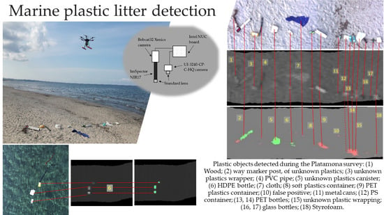
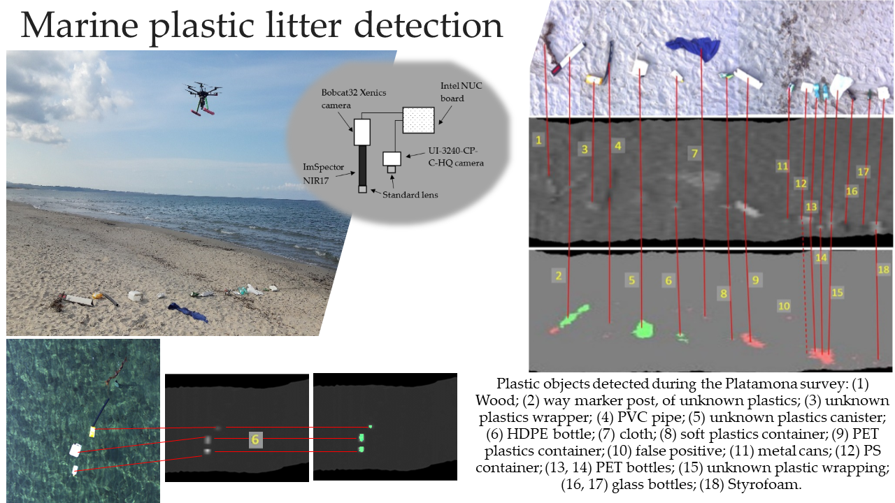
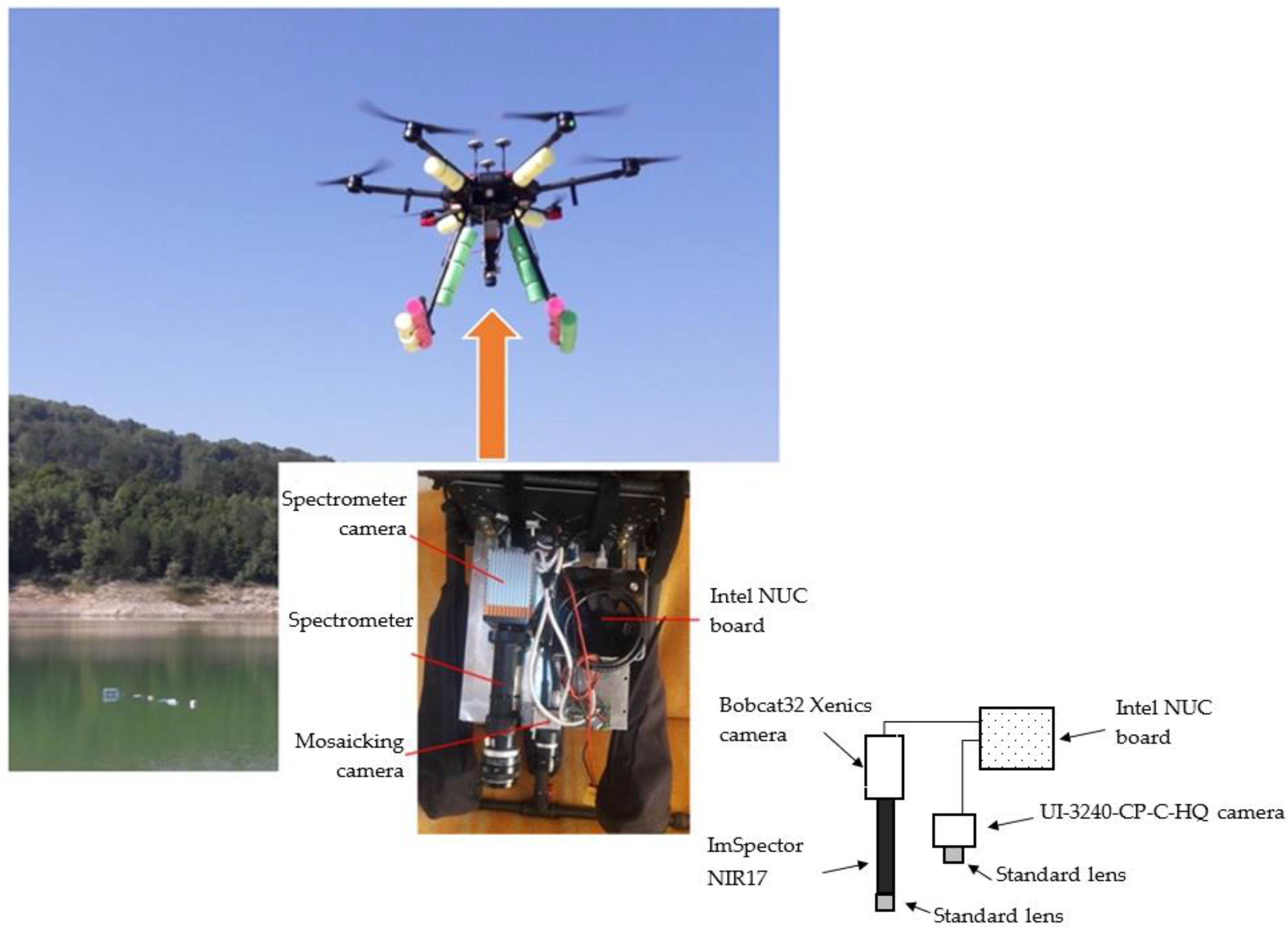
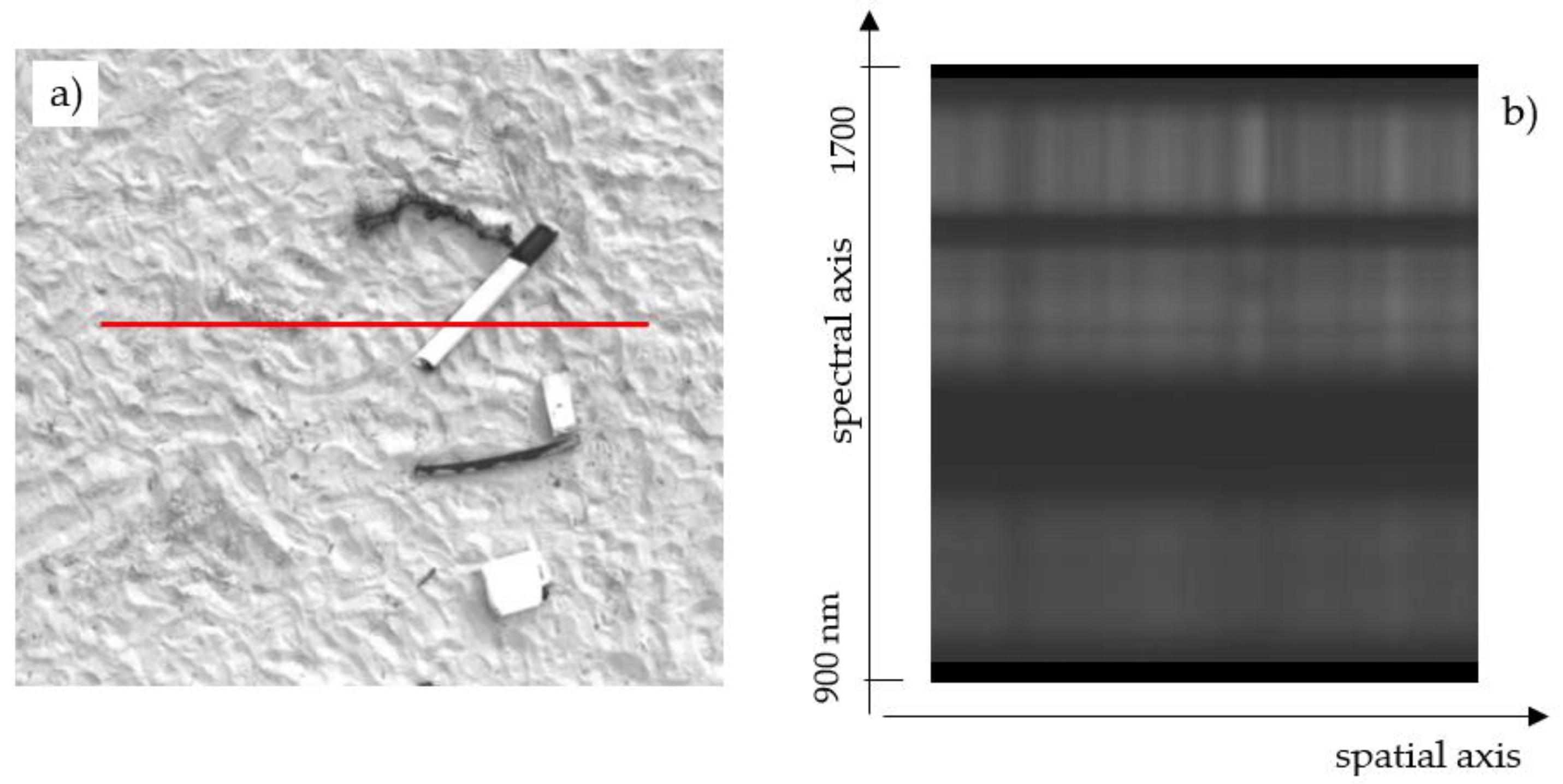
2.2. The Hyperspectral Imaging System, the UAV, and Onboard Instrumentation

The illustration reported in Figure 3 shows the DJI Matrice 600 drone employed for the measurement campaign and the hyperspectral device mounted on board. An Intel NUC single-board computer manages the synchronization, acquisition, and storage operations. In the platform design, the essential need for a device of reduced weight (about 2.5 kg in this non-optimized configuration) and low consumption (less than 100 W) has been carefully considered. In this way, the drone has a safe operating autonomy of more than 20 min.
A linear spectrometer ImSpector NIR17 OEM (Specim, Finland) is coupled with a SWIR camera (Bobcat 32 from Xenics, Belgium) of 256 × 320 pixel resolution (50 frames per second maximum acquisition frequency). The assembled spectral device (hereafter spectrometer camera) allows the acquisition of the hyperspectral information in the short-wave infrared range of the electromagnetic spectrum (900–1700 nm). Through a slit, the spectrometer captures a narrow line image of the target and disperses the light from each line pixel into a spectrum, orthogonally with respect to the line. Each spectral image impressed on the SWIR camera sensor has a spatial axis and a spectral axis. Spectral features of the entire target (i.e., the hyperspectral cube) can be obtained, in a so-called “push-broom” system, by acquiring images of the target while it is moving with respect to the spectral device or by moving the spectral device with respect to the target. In the latter case, the position of the spectrometer camera must be precisely recorded for post-flight georeferencing. GNSS (Global Navigation Satellite System) and IMU (Inertial Measurement Unit) are generally used for this purpose. This requires that the temporal resolution of the IMU system coincides with the frame rate used to acquire the spectral images and that the detected positions can be correlated with the corresponding images without ambiguity. The system developed in this study does not require a high-time-resolution and high-accuracy IMU because post-flight georeferencing is performed by employing a camera (UI-3240-CP-C-HQ from IDS, Germany, hereafter mosaicking camera) of 1280 × 1024 pixel resolution equipped with a standard lens. The spectrometer and mosaicking cameras are synchronized by hardware triggering and arranged with parallel optical axes. The acquisition frequency of both cameras is set equal to 16 fps.
Figure 4 displays one sample image acquired with the mosaicking camera and the corresponding image acquired simultaneously with the spectrometer camera. As shown in the figure, the image acquired with the mosaicking camera presents a portion of the area under investigation whereas the one acquired with the spectrometer camera contains the spectral features of the line image seen through the slit the spectrometer is equipped with. Such a line spans approximately the central part of the mosaicking camera field of view, even if it has a slightly smaller aperture size. Since several simultaneous images are acquired with the two cameras (i.e., the mosaicking and the spectrometer cameras) during each flight of the field survey, a mosaicking procedure is required to reconstruct the area under investigation and to properly georeference the line images acquired with the spectrometer camera. The in-house algorithms developed to achieve these goals are described in Section 2.3.
A few examples of spectra, taken on several points of the same scan, are shown in Figure 5. The y-axis of the plot presents Raw Digital Number units, corresponding to the sensor response recorded as 8-bit integers. It is apparent that, within the spectrum of the sensors, two bands show very low response. This is due to the fact that natural sunlight has very small content in these bands, due to atmospheric absorption [20]. Specific narrowband absorption of plastics is also not evident without calibration of the spectra.
The pixel width, projected to ground level, at a 10 m distance (the typical distance between sensors and target), is about 7 mm (transversally with respect to the flight direction), for the hyperspectral camera. Even though the same spacing between pixel centers in the directions across and along the flight path is desirable (in order to have the mosaic pixels approximately square), as the drone velocity (about 1 km/h) and the acquisition frequency (16 Hz) are taken into account, a spacing between hyperspectral lines in the flight direction of about 17 mm is obtained, suitable to identify objects a few cm wide. A lower flight speed would lead to an increase in time required for the survey and cause a distortion of the surveyed area due to attitude corrections in presence of wind. The use of a higher-frequency SWIR camera will permit an increase in flight speed, with a consequent reduction in the survey duration, while keeping pixels approximately square.

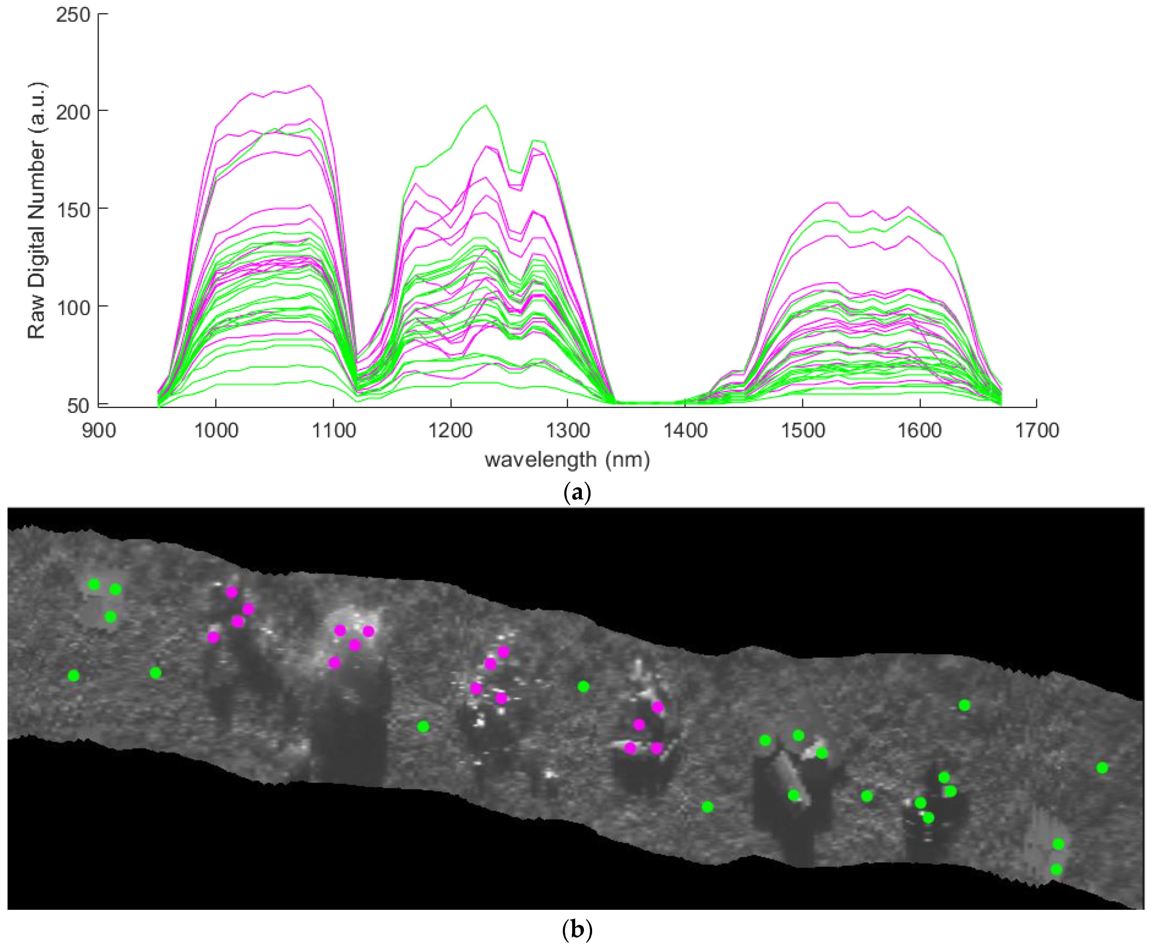
2.3. Hyperspectral Image Processing

The processing of the data simultaneously gathered by the mosaicking (visible images) and the spectrometer (spectral images) cameras is accomplished by performing the following steps.
(i)
Transformation of visible images taken over the scene into a single image obtained through a mosaicking procedure; translations, rotations, and scale changes between each couple of consecutive images are taken into account.
(ii)
Use of mosaicking results to correctly assign the line image acquired by the spectrometer within the investigated area.
(iii)
Construction of the hyperspectral cube (image of the scene at the different wavelengths).
To reconstruct the mosaic, the reciprocal positions of subsequent images of the acquired sequence, which usually consists of more than 150 images, are determined via the two-dimensional Fourier transform (2-DFFT) for detecting the maximum spatial correlation between image pairs. In fact, the rigid translation between a couple of images is related to the position of the peak of the cross-correlation among them. In the case of images acquired from an aerial vehicle, the mere translation between pairs of consecutive images is very unlikely. More generally, the images are affected by rotation and change of scale. Therefore, one image of the pair is rotated in the range of −5° to 5° with a 0.05° step, and the scale is modified relative to the original size of −6% to 6% with a step of 0.5%. The 2-DFFT procedure is iteratively applied to each image pair to select the image pair that maximizes the consistency of the luminosity. This methodology is suitable to process the large number of images detected by an aerial platform where it is assumed that no tilt occurs and that potential scale changes are the same in the two principal directions. As a matter of fact, the procedure adopted is equivalent to a four-parameter homographic transformation (similarity). Given the flight profile normally employed (nadiral images taken at approximately constant height and speed) and the requirements of the plastic detection survey (i.e., detection of objects, rather than topographic mapping), the orthorectification of the mosaic was not performed to keep computational cost low. Further details about the image-processing procedure are provided in [21,22]. The whole procedure is schematically illustrated in Figure 6, showing (a) a subset of images acquired by the mosaicking camera during one flight of the field survey (extracted from the set containing 154 images), (b) the result of the mosaicking procedure applied to the entire set of 154 images, and finally (c) the image at wavelength 1050 nm extracted from the reconstructed hyperspectral cube. The spatial resolutions of the mosaicking and spectrometer cameras are different and for this reason images shown in Figure 6b,c have different size and texture though they refer to the same area. The lower resolution of the spectrometer camera, i.e., Bobcat 32 from Xenics, is the reason why the image in Figure 6c appears blurred. Nevertheless, the objects clearly recognizable in Figure 6b can be located and identified.

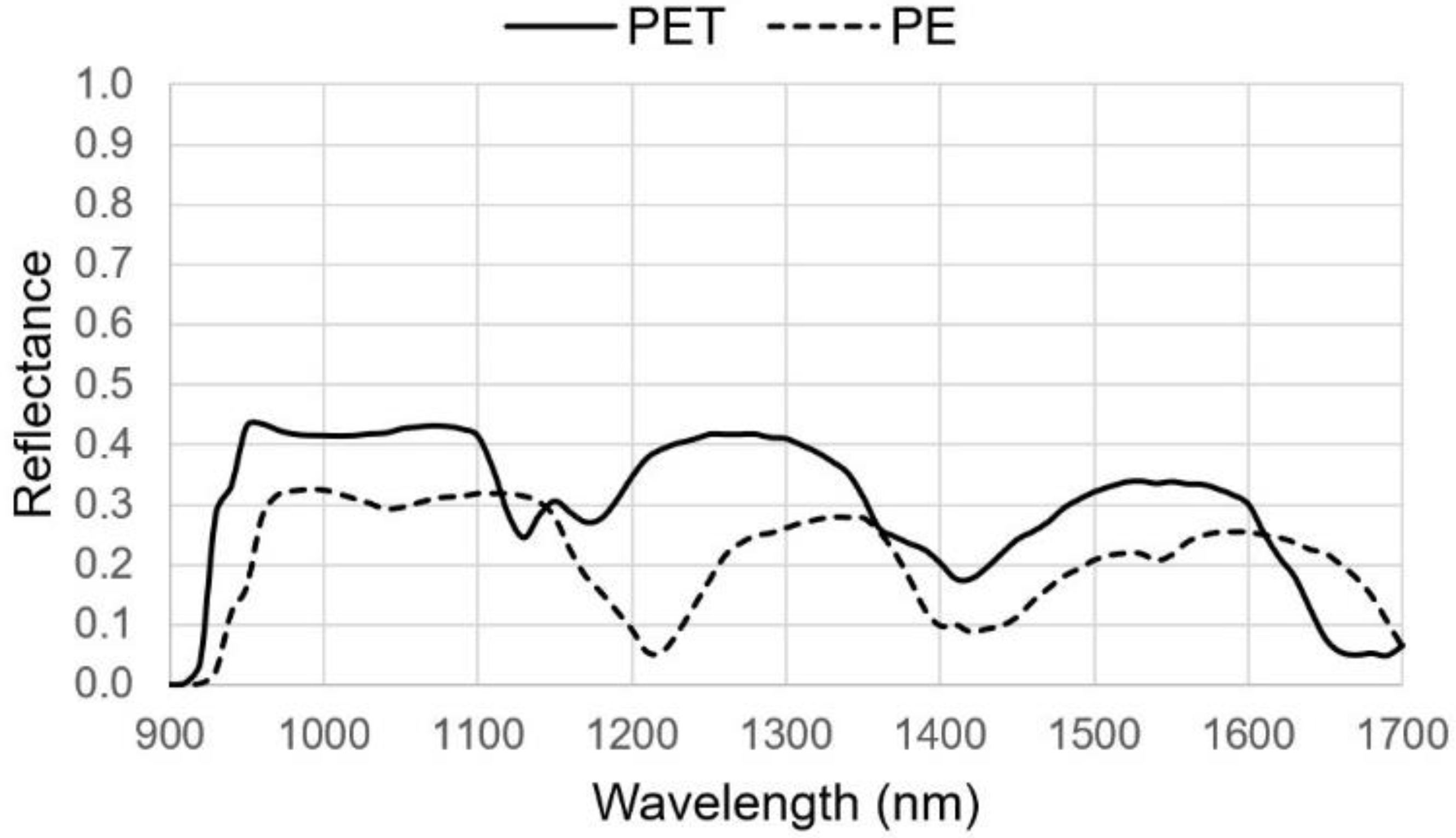
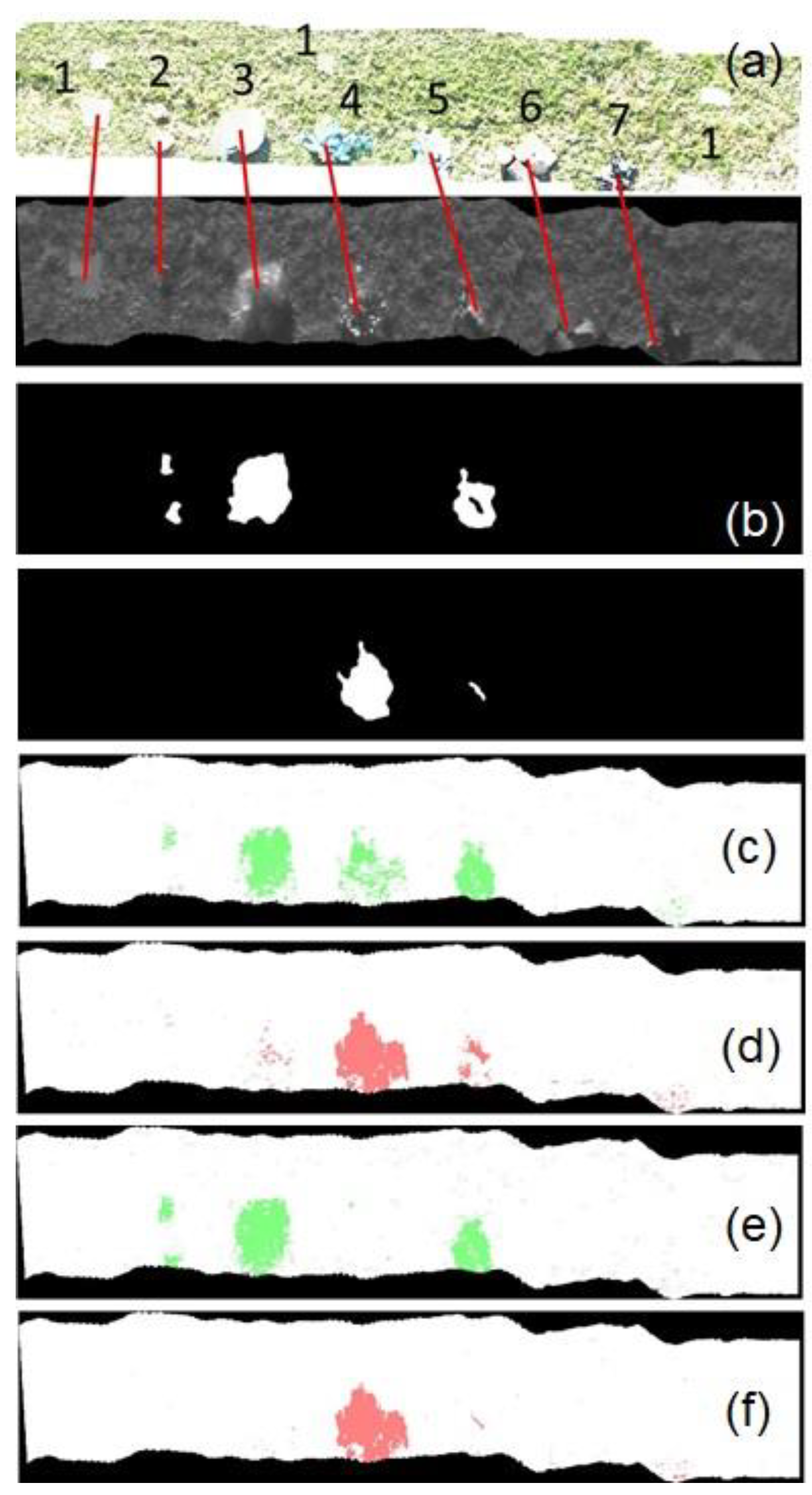
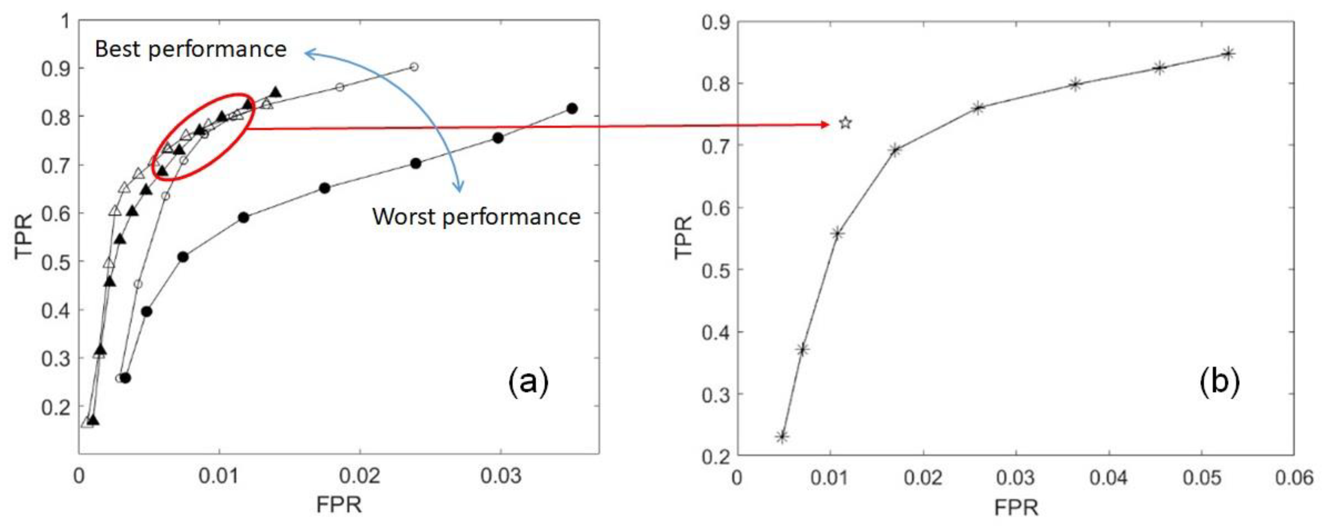
2.4. The Plastics Detection Algorithm

The wavelength spectrum of the hyperspectral sensor (900–1700 nm), projected onto the wide side of the SWIR sensor, is sensed into 320 bands, each about 2.5 nm wide. Since such a level of detail is not necessary for plastic discrimination [6], the original 320 bands were subsampled by ¼. A further selection was required in order to delete wavelength bands affected by absorption and scattering effects from atmospheric gases (mainly water vapor) and aerosols [20]. After such a selection, 38 10-nm bands, covering the ranges 950–1030 nm (band 1), 1110–1230 nm (band 2), and 1440–1590 nm (band 3) were retained and processed for plastics identification.
Hyperspectral data gathered within the three selected wavelength ranges were processed in order to obtain feature vectors for each spatial pixel. First of all, raw intensity values (elements of the hyperspectral cube, for each spatial pixel and wavelength) were normalized by computing the means of the raw vectors over the three band ranges: m1 for band 1, m2 for band 2, m3 for band 3. The feature vector was then assembled as follows: The first two components were m2/m1 and m3/m1. The following components were the intensities in band 2 normalized by dividing by m2 and the intensities in band 3 normalized by dividing by m3. The rationale for such choice is that characteristic absorptions of plastics polymers are not contained in band 1, but such a band is useful to set a common intensity mean level for pixels of different spectral properties, and possibly illuminated by changing overall radiation over time. Such operation has a similar effect as calibration and as taking reflectance ratios over two wavelengths (e.g., [6]). The first two components (means ratios) were included in the feature vector heuristically, because normalization would hide such information that may also be significant. Feature vector dimension is therefore 31 (2 mean ratios plus 29 intensity components), and the assembly of feature vectors over all spatial pixels may also be seen as a modified hyperspectral cube.
For the purpose of plastic waste detection, the major concern is not to determine which specific polymer a given object is made of, but to identify objects classified as a generic “plastics” class, as opposed to other objects classified as a “non-plastics” class. However, it can be conjectured that the “non-plastics” class is not convex and not linearly separable from the “plastics” class, because the wavelengths characterizing each polymer are not the same. Such situation is illustrated in Figure 7, showing feature vectors of PET, PE, and non-plastic samples from the learning set considered. It is apparent that the two polymers are characterized by different features, each distinguishable from non-plastic reflectors, which are more homogeneous among themselves in the response, despite being made of heterogeneous materials. Therefore, it is appropriate to classify each polymer separately, and then combine results. For such a task, linear classifiers are good candidates (e.g., [23]), with the advantage of simple and fast implementation. Therefore, after considering other parametric and non-parametric options, Linear Discriminant Analysis (LDA) [24] was chosen.
Multi-class classification was applied in this study, with the attention focused on PET or PE polymers (either low density LDPE or high density HDPE, which have essentially the same spectral behavior, differing only in density), taking into account that extension to a wider variety is immediate, given a good training sample. Single-polymer classes were combined into a compound “plastics” class by applying logical OR (set union) of the results.
Reducing the dimensionality of the feature vector improves the generalization ability of the classifier and allows for using a limited number of manually labeled training examples. For this purpose, the minimum-redundancy/maximum-relevance criterion [25] was employed. Such algorithm ranks feature vector components according to their relevance to the specific classification, jointly minimizing the inter-dependency between such variables, as a measure of the redundancy of an additional feature if added to the higher-rank features already selected in an iterative way. By cross-validating classifications in preliminary tests, a number of features between 5 and 10 resulted in being generally appropriate, and finally, 10 features were chosen in all the case studies described in Section 3. In fact, increasing the number of features did not appear to significantly impact either computation time or generalization ability. Table 1 indicates which bands were automatically selected as features by the algorithm, in order of relevance. Please notice that some wavelengths correspond to the main absorption peaks that can be deduced from Figure 1. The others do not appear, because they are located in bands where solar radiation is low. Furthermore, some adjacent wavelength groups appear in the list (e.g., 1200–1210–1220 nm and 1550–1560–1570 nm for PE, as well as 1540–1550–1560–1570 nm for PET).
The LDA classifiers were set up by training them using a training set of 279 samples, acquired in several preliminary flights in different conditions, and corresponding to 65, 80, and 134 manually selected spectra of PET, PE, and other materials (in particular grass, sand, water, besides wood, glass, etc.), respectively. Taking samples from data acquired on different scenes and in different environmental conditions guaranteed better generalization to new cases.
From this basic set, labeled into three classes (PET/PE/non-plastics), different derived training sets were built as follows:
  • Set 1 contains all samples of the original set, labeled into plastics (positive class) or non-plastics (negative class). This set reflects the final purpose of the detection.
  • Set 2 contains all samples of PE for the positive class, and all non-plastic samples in the negative class.
  • Set 3 is obtained in the same way as Set 2, for PET samples.
  • Set 4 contains all samples of PE for the positive class, and all non-plastic samples together with all PET samples in the negative class.
  • Set 5 is obtained in the same way as Set 4, but for PET samples in the positive class and PE samples in the negative one.
Sets 2 and 3 are meant to train the classifier to recognize a single polymer, and do not include samples of the other polymer, in order to treat it as a “don’t care” case, while Sets 4 and 5 forced the classifier to be more specific on a single polymer, and to consider the other as “negative” to detection.
In order to obtain a plastics/non-plastics classifier from the ones derived from Sets 2 and 3 or Sets 4 and 5, the positive results have to be combined by applying a set union operation over the positive response pixels of each classifier (i.e., a logical OR operation on the results, taking positive response as “true”). The final purpose of such operations is to compare the performance of the classifier obtained on Set 1 with the combined classifiers.

3. Results and Discussion

A distinctive feature of the developed algorithm was to separately identify PE and PET plastics, whose spectral properties differ from each other. For this reason, the classifiers obtained from Sets 2 and 4 for PE and from Sets 3 and 5 for PET were compared in order to test the conjecture that more specific classifiers (those obtained from Sets 4 and 5) are expected to work better. The results for all these cases are shown for a relevant example in Figure 8. As the ground-truth reference (material identification masks, Figure 8b) is obtained manually, the actual pixel count suffers from marginal error, but the comparison is not affected. It is apparent from Figure 8c–f that classifiers derived from Sets 4 and 5 perform significantly better than those obtained from Sets 2 and 3, as conjectured.
The performance of the classifiers was evaluated on the basis of ROC (Receiver Operating Characteristic) curves generated by using the discrimination threshold as a parameter, i.e., essentially the displacement of the separating plane from the origin. ROC curves are obtained by plotting true-positive rates (TPR—ratio of the number of vectors correctly classified as positive to the total number of positive cases considered) vs. false-positive rates (FPR—ratio of the number of vectors wrongly classified as positive to the total number of negative cases considered), i.e., by studying the trade-off between sensitivity (recognizing correctly most positive cases) and the complement to 1 of specificity (the latter being the case of recognizing most negative cases correctly) caused by accepting more or fewer cases as positive. For a perfect classifier, such curves should ideally be squashed to the upper-left corner of the graph (both sensitivity and specificity equal to 1, which is equivalent to TPR = 1 and FPR = 0), and the best parameter value is the one corresponding to the knee of the curve that is closest to the upper-left corner (at least when the risk of false positives is considered as important as the risk of false negatives).
Results for the classifier trained on Set 1 (all plastics together) were then compared with those for a classifier obtained by combining the results of classifiers trained on Sets 4 and 5, each of the latter sets with the optimum threshold. The results, in terms of ROC curves, are shown in Figure 9. Inspection of the figure reveals that the combined classifier performs significantly better than the all-plastics classifier trained on Set 1. This statement is apparent from the example displayed in Figure 10, where plastics have been more clearly identified by the combined classifier than by the one trained on Set 1. Indeed, these latter results correspond properly to the stated task of detecting a generic “plastics” class from everything else, while the distinction among polymers was instrumental to the optimal design of the classifier.
In order to optimize the sensor setup and to validate the methodologies previously described, the classifier, developed after the training procedure by using different sets of samples, was tested to check a controlled target consisting of an array of plastic and non-plastic litter laid on the grass and on bare earth. The target materials were inspected using the UAV-based remote-sensing system described in Section 2.2, according to the same procedure used for the main in situ remote-sensing campaign. Results are shown in Figure 11 and Figure 12: For both experiments, the output of the hyperspectral image processing clearly reports the shape of objects made of PE (in green) and PET (in pink), neglecting all the non-plastic objects and those made of other plastic typologies. The objects appearing in blue were identified as plastics, but the algorithm responded positively both to PE and PET.
It is interesting to notice that Polypropylene (PP), which was not included in the training set, is actually efficiently recognized as PE or both as PE and PET. From the point of view of recognizing plastics, this means that training a specific classifier for PP is not actually necessary.
The validated procedure was applied to the hyperspectral data gathered on the seashore of Sassari (Sardinia, Italy). Since at the time of the in-situ inspections at the Platamona and Porto Ferro sites almost no litter was found either on the beach or in the sea water facing the beach, targets were prepared on site, through several plastic and non-plastic objects attached in line, using a rope, to ensure their removal at the end of the mission, and an anchor at one extremity, to provide stability of the assembly. Bottles were empty to prevent a possible sinking of samples. These targets were positioned both on the sandy beach and in the sea water at least 20 m away from the coastline.
Some representative results are displayed in Figure 13, Figure 14 and Figure 15. Figure 13 displays an array of five objects floating on the sea (Platamona beach), clearly visible in the image on the left. The final results obtained from the application of the detection algorithm are shown in the image in the bottom-right corner: Two PE objects have been correctly identified (and displayed in green), while the other objects and the background are neglected by the classifier, thus they appear as dark in the image. In the top-right corner, the same figure shows the image, extracted from the hyperspectral cube, corresponding to the wavelength 1010 nm from which, at a different extent, all the objects are distinguishable. The comparison of the two images on the right clearly shows the role of the trained classifier able to discern the type of plastics and then to highlight only the selected type of polymer (PE).
The same methodology was applied to identify and distinguish plastic objects on the sand of Platamona and Porto Ferro beaches, whose results are shown in Figure 14 and Figure 15. In particular, Figure 14 displays the visible image of a litter assembly on the sand, its spectral (at wavelength 1010 nm) counterpart, and the output provided by the classifier, highlighting, using the conventional colors of green and pink, PE and PET materials, respectively. Figure 15 provides a further example of the identification of PE and PET objects on the sandy beach. Two separate scans of the hyperspectral sensor are shown near a mosaic of several images of the visible image sensor. It is worth noting that, even though the background is less favorable, as compared to the sea water (featuring a very low reflectance in the SWIR wavelength range), the type and shape of target objects are correctly identified. Finally, inspection of figures confirms that in all situations, the developed system performed remarkably well, also detecting small PE and PET objects (#1 and #2 in Figure 15) that were incidentally present on the beach and not placed there on purpose.
An interesting characteristic of a UAV-based remote-sensing system for macroplastics identification is related to the possibility of real-time detection of the plastic litter during the flight survey, particularly useful especially for floating litter. In fact, such litter is continuously moving, so that detection performed online permits the immediate warning or logging of its position for later use, taking into account winds and currents. As discussed in Section 2.3, hyperspectral cubes were reconstructed using the mosaic of visible images acquired simultaneously, and based on such cubes, static materials classification maps were reconstructed. However, it is to be noted that mosaicking is not a well-posed problem in the case of floating litter, because object positions, which should be assumed constant, actually may not be. There are situations where mosaicking is impossible, for instance on an object-free perfectly smooth water surface, where no significant points can be found in images at all, or in fast-moving water, where objects are rapidly displaced and the background is not stable. Thanks to the very low computation load of the detection algorithm, real-time detection can indeed be performed even by a very low-performance embedded computer carried on board the drone.
Examples of short video sequences, gathered during both the Platamona and Porto Ferro surveys, have been reported as Supplementary Material to this paper, and some snapshots of the video clips documenting real-time detection are reported in Figure 16. A yellow line overlapped to the framed scene indicates the position of the hyperspectral sensor line, relative to the visible image; when PE or PET objects are intercepted by the yellow line during a real-time inspection, a red bar appears in the upper part of the frame to indicate a positive response of the plastics detector, otherwise a green bar is displayed (to indicate a negative response).

4. Conclusions

UAV-based remote-sensing systems have a great potential for the detection and identification of marine plastic litter. It was demonstrated in this research that the identification of the plastic types may derive from a process involving the mosaicking of gathered images, the hyperspectral image processing, and the application of a trained algorithm able to discern the spectral properties of each polymer. This process was implemented by training the algorithm using different sets of samples in order to identify the classifier most suitable for PE and PET plastic detection and verified by inspecting plastic and non-plastic controlled targets.
The measurement and processing chain was used for the remote-sensing inspection of the seashores of Sassari (Sardinia, Italy). Tests performed on the sandy beaches and in the seawater were able to distinguish both the shape and the typology of macroplastics (at the moment PE and PET, but in principle the method can be applied to a large cohort of different polymers), even in a real-time application. This last characteristic permits an immediate detection of floating plastics, making it possible to remove them or to trace and monitor their position for a successive intervention. Compared to current methods for the identification of marine plastic litter by remote sensing, the methodology presented in this paper has the advantage of being completely automatic in its field application, and capable of real-time operation.
The developed plastics detection algorithm is obtained by supervised learning of a linear classifier. Such a methodology proved quite effective, and the linear classifier has the advantage of requiring very little computation resources, so that it can be implemented even on a tiny board computer operating in real time on board a drone. Other types of more sophisticated machine learning frameworks do not seem necessary, since indeed the most work-intensive task required in this context is the manual labeling of training samples, which cannot be automatized. Nevertheless, since neural and deep-learning architectures are envisaged in the near future for Internet of Things and edge-computing, as a future development of this work, the same data might be processed using a neural architecture to assess possible advantages of such learning machines.

Supplementary Materials

The following are available online at https://www.mdpi.com/article/10.3390/rs13081557/s1, Video S1: Balsi et al._real-time-detection.mp4.

Author Contributions

Conceptualization and methodology, M.B., M.M., V.C., and G.T.; software, M.B. and M.M.; validation, M.B. and M.M.; investigation, M.B., M.M., V.C., and G.T.; writing, M.B., M.M., and G.T.; funding acquisition, V.C. All authors have read and agreed to the published version of the manuscript.

Funding

This research has been partially funded by the Region of Sardinia (Italy) under the project TEMPUS POR/FESR Sardegna 2014–2020 Asse 1 Azione 1.1.3 Strategia 2.

Institutional Review Board Statement

Not applicable.

Informed Consent Statement

Not applicable.

Data Availability Statement

The data presented in this study are available on request from the corresponding author.

Conflicts of Interest

The authors declare no conflict of interest.

References

  1. Gall, S.C.; Thompson, R.C. The impact of debris on marine life. Mar. Pollut. Bull. 2015, 92, 170–179. [Google Scholar] [CrossRef]
  2. Maximenko, N.; Corradi, P.; Law, K.L.; Van Sebille, E.; Garaba, S.P.; Lampitt, R.S.; Galgani, F.; Martinez-Vicente, V.; Goddijn-Murphy, L.; Veiga, J.M.; et al. Toward the integrated marine debris observing system. Front. Mar. Sci. 2019, 6, 447. [Google Scholar] [CrossRef] [Green Version]
  3. Martínez-Vicente, V.; Clark, J.R.; Corradi, P.; Aliani, S.; Arias, M.; Bochow, M.; Bonnery, G.; Cole, M.; Cózar, A.; Donnelly, R.; et al. Measuring marine plastic debris from space: Initial assessment of observation requirements. Remote Sens. 2019, 11, 2443. [Google Scholar] [CrossRef] [Green Version]
  4. Garaba, S.P.; Acuña-Ruz, T.; Mattar, C.B. Hyperspectral longwave infrared reflectance spectra of naturally dried algae, anthropogenic plastics, sands and shells. Earth Syst. Sci. Data 2020, 12, 2665–2678. [Google Scholar] [CrossRef]
  5. Van Den Broek, W.H.A.M.; Wienke, D.; Melssen, W.J.; Buydens, L.M.C. Plastic material identification with spectroscopic near infrared imaging and artificial neural networks. Anal. Chim. Acta 1998, 361, 161–176. [Google Scholar] [CrossRef]
  6. Moroni, M.; Mei, A.; Leonardi, A.; Lupo, E.; La Marca, F. PET and PVC separation with hyperspectral imagery. Sensors 2015, 15, 2205–2227. [Google Scholar] [CrossRef]
  7. Balsi, M.; Esposito, S.; Moroni, M. Hyperspectral characterization of marine plastic litters. In Proceedings of the 2018 IEEE International Workshop on Metrology for the Sea, Learning to Measure Sea Health Parameters (MetroSea), Bari, Italy, 8–10 October 2018; pp. 28–32. [Google Scholar]
  8. Colomina, I.; Molina, P. Unmanned aerial systems for photogrammetry and remote sensing: A review. ISPRS J. Photogramm. Remote Sens. 2014, 92, 79–97. [Google Scholar] [CrossRef] [Green Version]
  9. White, J.C.; Coops, N.C.; Wulder, M.A.; Vastaranta, M.; Hilker, T.; Tompalski, P. Remote sensing technologies for enhancing forest inventories: A review. Can. J. Remote Sens. 2016, 42, 619–641. [Google Scholar] [CrossRef] [Green Version]
  10. Torresan, C.; Berton, A.; Carotenuto, F.; Di Gennaro, S.F.; Gioli, B.; Matese, A.; Miglietta, F.; Vagnoli, C.; Zaldei, A.; Wallace, L. Forestry applications of UAVs in Europe: A review. Int. J. Remote Sens. 2017, 38, 2427–2447. [Google Scholar] [CrossRef]
  11. Zhang, C.; Kovacs, J.M. The application of small unmanned aerial systems for precision agriculture: A review. Precis. Agric. 2012, 13, 693–712. [Google Scholar] [CrossRef]
  12. Arnó, J.; Martínez-Casasnovas, J.A.; Ribes-Dasi, M.; Rosell, J.R. Review. Precision viticulture. Research topics, challenges and opportunities in site-specific vineyard management. Span. J. Agric. Res. 2009, 7, 779–790. [Google Scholar] [CrossRef] [Green Version]
  13. Tanda, G.; Chiarabini, V. Use of multispectral and thermal imagery in precision viticulture. J. Phys. Conf. Ser. 2019, 1224, 012034. [Google Scholar] [CrossRef]
  14. Tanda, G.; Balsi, M.; Fallavollita, P.; Chiarabini, V. A UAV-based thermal-imaging approach for the monitoring of urban landfills. Inventions 2020, 5, 55. [Google Scholar] [CrossRef]
  15. Toth, C.; Józków, G. Remote sensing platforms and sensors: A survey. ISPRS J. Photogramm. Remote Sens. 2016, 115, 22–36. [Google Scholar] [CrossRef]
  16. Goddijn-Murphy, L.; Peters, S.; van Sebille, E.; James, N.A.; Gibb, S. Concept for a hyperspectral remote sensing algorithm for floating marine macro plastics. Mar. Pollut. Bull. 2018, 126, 255–262. [Google Scholar] [CrossRef] [Green Version]
  17. Garaba, S.P.; Aitken, J.; Slat, B.; Dierssen, H.M.; Lebreton, L.; Zielinski, O.; Reisser, J. Sensing ocean plastics with an airborne hyperspectral shortwave infrared imager. Environ. Sci. Technol. 2018, 52, 11699–11707. [Google Scholar] [CrossRef]
  18. Topouzelis, K.; Papakonstantinou, A.; Garaba, S.P. Detection of floating plastics from satellite and unmanned aerial systems (Plastic Litter Project 2018). Int. J. Appl. Earth Obs. Geoinf. 2019, 79, 175–183. [Google Scholar] [CrossRef]
  19. Topouzelis, K.; Papageorgiou, D.; Karagaitanakis, A.; Papakonstantinou, A.; Ballesteros, M.A. Remote sensing of sea surface artificial floating plastic targets with Sentinel-2 and unmanned aerial systems (Plastic Litter Project 2019). Remote Sens. 2020, 12, 2013. [Google Scholar] [CrossRef]
  20. Gao, B.C.; Montes, M.J.; Davis, C.O.; Goetz, F.H. Atmospheric correction algorithms for hyperspectral remote sensing data of land and ocean. Remote Sens. Environ. 2009, 113, S17–S24. [Google Scholar] [CrossRef]
  21. Moroni, M.; Dacquino, C.; Cenedese, A. Mosaicing of hyperspectral images: The application of a spectrograph imaging device. Sensors 2012, 12, 10228–10247. [Google Scholar] [CrossRef]
  22. Moroni, M. Vegetation monitoring via a novel push-broom-sensor-based hyperspectral device. J. Phys. Conf. Ser. 2019, 1249, 012007. [Google Scholar] [CrossRef]
  23. Ferreira, M.P.; Zortea, M.; Zanotta, D.C.; Shimabukuro, Y.E.; Souza Filho, C.R. Mapping tree species in tropical seasonal semi-deciduous forests with hyperspectral and multispectral data. Remote Sens. Environ. 2016, 179, 66–78. [Google Scholar] [CrossRef]
  24. Fisher, R.A. The use of multiple measurements in taxonomic problems. Ann. Eugen. 1936, 7, 179–188. [Google Scholar] [CrossRef]
  25. Peng, H.C.; Long, F.; Ding, C. Feature selection based on mutual information: Criteria of max-dependency, max-relevance, and min-redundancy. IEEE Trans. Pattern Anal. Mach. Intell. 2005, 27, 1226–1238. [Google Scholar] [CrossRef]
Figure 1. Spectral signatures of plastics typologies measured in laboratory-controlled conditions (Balsi et al., [7]).
Remotesensing 13 01557 g001
Figure 2. Images of the inspected sites for the field campaigns. Satellite and ground-based photographs of Platamona and Porto Ferro, Sardinia, Italy.
Remotesensing 13 01557 g002
Figure 3. Drone employed for the measurement campaigns and details of the instrumentation onboard.
Remotesensing 13 01557 g003
Figure 4. (a) Sample image acquired with the mosaicking camera; (b) simultaneous image acquired with the spectrometer camera, containing the spatial/spectral info of the line image drawn in red over the visible image.
Remotesensing 13 01557 g004
Figure 5. (a) Examples of typical raw spectra of pixels corresponding to plastics (magenta), namely PE and PET materials, and non-plastics (green), namely wood, glass, floor tiles, grass-covered ground; ordinates are in Raw Digital Number units, corresponding to the sensor response recorded as 8-bit integers. (b) Hyperspectral cube layer for wavelength 1010 nm: superimposed magenta points correspond to plastics spectra of panel (a), green points to non-plastics spectra.
Remotesensing 13 01557 g005
Figure 6. (a) Selection of images acquired during one of the flights above the seashore; (b) result of the mosaicking procedure applied to 154 images; (c) image at wavelength 1050 nm extracted from the corresponding hyperspectral cube.
Remotesensing 13 01557 g006
Figure 7. (a) Feature vectors of PET (blue), PE (red), and non-plastic samples (black) from the training set; (b) difference of the means of vectors from panel (a): Diamonds: (PET)- (non-plastics); circles: (PE)- (non-plastics).
Remotesensing 13 01557 g007
Figure 8. (a) Identification of materials. Panel above is a mosaic of visible-spectrum images, below the corresponding hyperspectral cube layer for wavelength 1010 nm; (1) white floor tiles; (2) LDPE wrapping bags; (3) LDPE wrapping sheet; (4) PET bottles (5) HDPE bottles; (6) wood; (7) glass bottles. Background is low grass. (b) Manually drawn masks for PE (above) and PET (below): Positive in white, negative in black. Classification results for classifiers trained on (c) Set 2, (d) Set 3, (e) Set 4, (f) Set 5: Positive in pink for PET, green for PE, negative in white. Optimized thresholds were used. It is apparent that the results obtained on the latter two sets are “cleaner” (more specific) and cover the areas better (more sensitive).
Remotesensing 13 01557 g008
Figure 9. True Positive Rates vs. False Positive Rates. (a) ROC curves for classifiers trained on Set 2 (black circles); Set 4 (empty circles); Set 3 (black triangles); Set 5 (empty triangles). The curves for Sets 3 and 5 (empty markers) are both closer to the upper-left corner than those for Sets 2 and 4 (black markers), respectively, denoting better performance. (b) ROC curve for Set 1 (all plastics together), compared with the optimal two-stage classifier (Set 4 OR Set 5 results for optimal parameters—isolated star), which is closer to the upper-left corner of the figure than any point of the all-plastics ROC curve.
Remotesensing 13 01557 g009
Figure 10. (a) Result of classification for the classifier trained on Set 1 (all plastics together); (b) combined classifier (Set 4 OR Set 5): Green denotes detected PE, pink denotes PET, and blue points where both classifiers respond positively; (c) manually drawn materials identification mask for all plastics.
Remotesensing 13 01557 g010
Figure 11. Detection of objects over grass: (1) Plastic crate; (2) PET container; (3) cardboard; (4) PS tray; (5) aluminum foil; (6) floor tile; (7) PET container; (8) PET bottle; (9) brick; (10) wood; (11) PET container; (12) HDPE bottle; (13) PET bottle; (14) metal can; (15) plastic thread; (16) PET tray; (17) wood; (18) and (19) glass bottles; (20) PET bottle; (21) Styrofoam floater; (22) and (23) PET bottles; (24) HDPE bottle; (25) PET bottle; (26) iron container (with pasted label); (27) floor tile. Color codes as in Figure 10.
Remotesensing 13 01557 g011
Figure 12. Detection of objects over bare earth: (1) PET bottles; (2) unknown plastics container; (3) Polypropylene (PP) containers; (4) unknown plastics container; (5) PP containers; (6) floor tile; (7) LDPE bags; (8) HDPE bottles. Color codes as in Figure 10.
Remotesensing 13 01557 g012
Figure 13. Detection of plastic objects in the sea of Platamona beach: (1) HDPE bottle; (2) unknown plastics canister; (3) metal-coated wrapper; (4) PVC pipe; (5) wood. Green denotes detected PE. As the PVC pipe is black, response in the SWIR spectrum is almost null, just as water, that appears completely dark throughout the sensor bandwidth.
Remotesensing 13 01557 g013
Figure 14. Detection of plastic objects on Platamona beach: (1) Wood; (2) way marker post, of unknown plastics; (3) unknown plastics wrapper; (4) PVC pipe; (5) unknown plastics canister; (6) HDPE bottle; (7) cloth; (8) soft plastics container; (9) PET plastics container; (10) false positive; (11) metal cans; (12) PS container; (13, 14) PET bottles; (15) unknown plastic wrapping; (16, 17) glass bottles; (18) Styrofoam.
Remotesensing 13 01557 g014
Figure 15. Detection of plastic objects on Porto Ferro beach: (1) Small piece of a plastic football; (2) unidentified debris; (3) PE wrappers; (4) PET bottles; (5) HDPE bottles; (6) Styrofoam floater. The mosaic representing the scene under investigation was obtained from visible spectrum images taken during several passes over the area, the red boxes indicate approximate areas covered by the hyperspectral cubes processed.
Remotesensing 13 01557 g015
Figure 16. Snapshots from real-time detection. Yellow lines indicate the position and field-of-view of the hyperspectral sensor line, relative to the visible image. A red or green bar indicates positive or negative response of the plastics detector, respectively. (a) PET bottles on grass; (b) Platamona; (c,d) Porto Ferro.
Remotesensing 13 01557 g016
Table 1. Most relevant wavelengths chosen automatically for polymer discrimination.
Rank OrderPE Wavelength [nm]PET Wavelength [nm]
111501620
215601550
312101180
412701570
515701510
611801270
715501560
812201220
912001540
1012501240
Publisher’s Note: MDPI stays neutral with regard to jurisdictional claims in published maps and institutional affiliations.

