Abstract
This paper reports a semi-automated workflow for detection and quantification of forest damage from windthrow in an Alpine region, in particular from the Vaia storm in October 2018. A web-GIS platform allows to select the damaged area by drawing polygons; several vegetation indices (VIs) are automatically calculated using remote sensing data (Sentinel-2A) and tested to identify the more suitable ones for quantifying forest damage using cross-validation with ground-truth data. Results show that the mean value of NDVI and NDMI decreased in the damaged areas, and have a strong negative correlation with severity. RGI has an opposite behavior in contrast with NDVI and NDMI, as it highlights the red component of the land surface. In all cases, variance of the VI increases after the event between 0.03 and 0.15. Understorey not damaged from the windthrow, if consisting of 40% or more of the total cover in the area, undermines significantly the sensibility of the VIs to detecting and predicting severity. Using aggregational statistics (average and standard deviation) of VIs over polygons as input to a machine learning algorithm, i.e., Random Forest, results in severity prediction with regression reaching a root mean square error (RMSE) of 9.96, on a severity scale of 0–100, using an ensemble of area averages and standard deviations of NDVI, NDMI, and RGI indices. The results show that combining more than one VI can significantly improve the estimation of severity, and web-GIS tools can support decisions with selected VIs. The reported results prove that Sentinel-2 imagery can be deployed and analysed via web-tools to estimate forest damage severity and that VIs can be used via machine learning for predicting severity of damage, with careful evaluation of the effect of understorey in each situation.
1. Introduction
High severity natural disturbances can significantly alter the structure and morphology of forest landscape [1,2,3]. The damage assessment, generally evaluated using severity classes, has been usually carried out through field surveys.
Wind is the main disturbance agent affecting European forests, being responsible for more than 50% of all damage by volume [4]. The damage from fire and windstorms have been increasing over the past centuries, and they are likely to continue to increase in the next future [5,6]. According to Gregow et al. [7], windstorms that affected the Central and Northern European forests in the last decade were stronger than the ones that occurred before 1990. Moreover, in the period between 1980–2010, the impact on forest areas, considering the same amount of biomass, was 3–4 times higher than that registered in the period between 1950–1980. Part of this increase might be due to climate change [8], but most of it is high likely due to factors related to the current stand conditions of the European forests [9].
The cost of such damage can be very high in economic terms (e.g., €6 billion in France from storms Lothar and Martin in 1999, and around €1.9 billion in Sweden after the storm Gudrun in 2005) [10]. Further added impact on local communities and forest ecosystems must be also considered. On 29 October 2018, the Vaia storm and flood event hit North-Eastern Italy, causing damage to forests mainly located in Alpine areas of the following regions: Veneto, Trentino-South Tyrol, Friuli Venezia Giulia, and Lombardy. The average and maximum value of the high-intensity rainfall was 335 mm and 519 mm, respectively, over a single day, and the wind had peak wind speeds recording close to 200 km h−1 (SE direction). The storm caused extensive forest damage, completely uprooting trees in large areas or severely damaging forests of about 42,500 ha, with a first estimated volume of timber loss of 8.5 million cubic metres [11,12,13]. Some forest stands were completely blown down, probably because the wind was funneled into the Alpine valleys and increased speed by the orography [14], and the characteristics of forests make the stands more susceptible to windthrow (simple structure, monolayered, and monospecific Norway spruce stands). The Copernicus Emergency Mapping system reports only about 4000 ha of damaged areas, about 10% of the affected area, due to cloud cover presence in the optical images used for mapping [15]. Following the Vaia storm, the impacted regions assessed the forest damage by means of aerial photographs and very high-resolution optical satellite images with data from field surveys. Manual area digitalization was adopted, which resulted in complex interpretation due to mixed interpretations of degree of damage, in particular where many trees were left standing. In addition, the definition of boundaries are subjective, as often there is not a clearly defined margin between damaged and untouched forest.
Major challenges for forest-related scientific investigation are related to the analysis of present and future vulnerabilities of forest socio-ecological systems as well as to translate associated risks and their outcomes into forest management, policy, and governance recommendations. In a period of changes, the governance and management of forests require innovation, making the role of research more important than ever. Remote sensing can supply timely and new information to the public administration and stakeholders involved in forest management. The change detection after a natural disturbance needs pre-event information, but these are not always available and not always complete. Data derived from remote sensing time series are widely used in change detection analyses concerning habitats, forest health, degradation of natural resources, biotic and abiotic disturbances, or forest recovery [16]. Remote sensing data can provide efficient decision support by supplying an overview of the land-use/land-cover (LULC) scenario over time. Satellite imagery supports the creation of thematic maps that cover large regions to help public administration and stakeholders plan efficient forest management [17]. On the other hand, remote sensing processing requires specialized skills for correct imagery acquisition, model calibration, and analysis.
Processing satellite imagery can now be done through cloud-based analysis platforms, such as Google Earth Engine [18]. Cloud-based platforms automate several time-consuming pre-processing steps such as image acquisition, quality masking, cloud-filtering, and analysis. The downside is that operators are in the so-called “vendor-locked” position. In this specific investigation, a custom cloud-based remote cluster was used to develop a web-GIS platform for custom automation of satellite image analysis. This platform allows real-time calculation of vegetation indices (VIs) over time-series of image data. Results from analyses through this processing pipeline are presented relative to using VIs for assessment of the estimation of degree of damage, expressed in percent.
Vegetation indices have been widely investigated for forestry applications and also for investigating Vaia damage localization [19]. One of the more commonly used VIs, the normalized difference vegetation index (NDVI), is calculated as the normalized ratio of the difference between the near-infrared band and the red band and is used for monitoring the vegetation canopy response to stress and other factors that change absorption of the red or infrared part of the spectrum. Normalized indices limit noise due to changes in the irradiance condition e.g., to clouds, different sun angles, atmospheric condition or topography [20] and are applied to analyze seasonal and annual trends [21]. It must be noted that VIs depend strongly also on the phenology, i.e., the growing stage, not only on disturbance and stress factors induced by climate change or pathogen attacks. NDVI has a non-linear response, in sparsely vegetated areas where the background reflectance of the red spectral band increases [22,23,24]. Over densely vegetated areas, NDVI enhances the low ratio values while compressing higher ratio values. The enhanced vegetation index (EVI) was created to correct the background effect using a soil adjustment factor, L, and correcting the red band with blue band coefficients, C1 and C2 [23]. In the windthrow-damaged area, the forestry patch is sparse and many trunks lie on the ground. Hence, EVI has been tested to reduce the noise effect of the canopy background. A damaged forest, with weakened, stressed, and fallen trees as in Figure 1, can be the optimal habitat for forest pests like the European spruce bark beetle (Ips typhographus) [25].
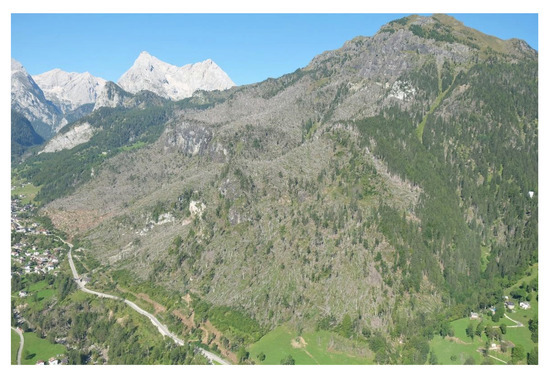
Figure 1.
A damaged forest hit by the Vaia windstorm in the Agordino region.
The stages of the pest attack are the green-attack, red-attack, and grey-attack, where stressed vegetation loses foliage, increases the visible red spectral component, and decreases the near-infrared response [26]. In the green-attack, the foliage looks unchanged. Thus, it is difficult to identify, and the moisture decreases in the sapwood [27]. The red-stage happens the next year and the foliage turns yellow and red. Finally, the tree loses needles, and turns to grey. The grey stage has been studied with NDVI [28], but several studies have focused on the red stage applying the RGI index [29,30,31].
The relative greenness index (RGI) is an index of anthocyanin content [32], and it takes into consideration the response of the red band over the green band. Study results on this index bring evidence of a high correlation coefficient, from 0.7 to 0.9, between pixels covered with red-stage pest attack and the tree crown using a very high spatial resolution imagery e.g., ~1 m resolution or less. The epidemic red stage was studied in Canada using Landsat-TM imagery and applying the enhanced wetness difference index (EWDI) in a mixed forest [33]. The EWDI is calculated by subtracting the tasseled cap wetness index [34] of two images in different years. Again, the red-stage attack was studied by [35] using the normalized difference moisture index (NDMI). Wilson and Sader [36] found higher accuracies of NDMI over NDVI in change detection of forest harvest. Biotic and abiotic disturbances were studied considering the red-edge chlorophyll indices (CI) and NDVI for estimating the temporal change in leaf chlorosis and defoliators in [37].
Previous scientific literature supports further investigation to understand the accuracy of modelling damage from windthrow using vegetation indices, to identify those that provide optimal results over mountain regions characterized by an Alpine environment. The specific goal of this paper is to report on results of testing NDVI, EVI, RGI, EWDI, NDMI, and CI indices through machine learning and to identify which indices are more suitable for quantifying damage in areas in the Agordino forest hit by the Vaia storm, considering also the disturbance and recovery stage. The results have been integrated into a web-GIS application to support the public administration and stakeholders involved in forestry management.
2. Materials and Methods
2.1. Study Area
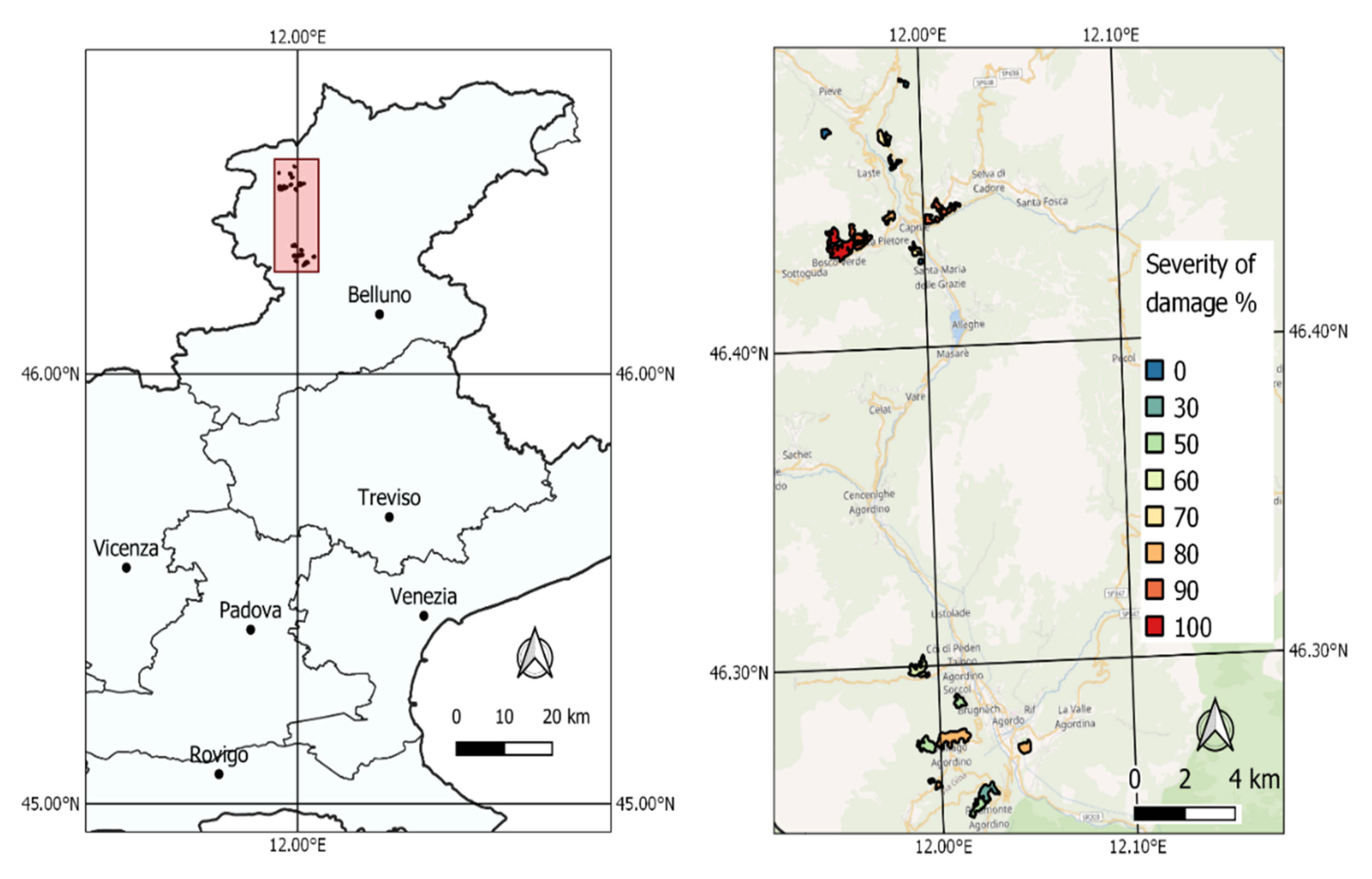
The study area is located in the upper and middle Cordevole Valley, named Agordino. Here, the forests were severely damaged by the Vaia storm, which affected almost 4000 ha (6% of the area) with more than 600,000 m3 of windthrown timber. Consequently, 22 testing areas (Figure 2), representative of a gradient of severity, aspect, and slope, were inspected between June and September 2019. The size of the testing areas ranges between 1 ha and 61.58 ha.
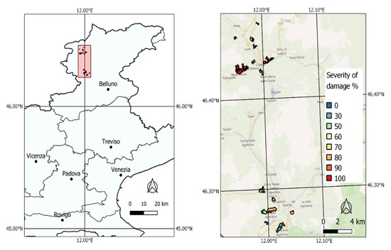
Figure 2.
Location of 22 surveyed areas, with information on damage severity, located in the Agordino region.
2.2. Field Survey
The severity was assessed by determining the canopy cover loss by visual interpretation and validation by experts. First, interpretation was done using high-resolution orthoimagery from aerial surveys (acquired in 2019), determining the boundaries of the area considered damaged and providing a value of severity (canopy loss) on a scale from 0 to 100. The second step consisted of a visual inspection directly on site, validating or changing the severity class assigned in the first step.
The field survey consisted of visual inspection of the 22 plots reporting (i) the severity in the percentage of fallen trees; a description of the damage with percentages of (ii) residual canopy cover, (iii) understorey, (iv) overall health index, and (v) crown status of standing trees. Visual inspection means that expert personnel physically went in the area and validated the initial severity assessment for each plot. The survey is necessary to assess the forest condition, and to correlate the ground truth with the values of VIs that were derived from Sentinel-2 imagery. The fieldwork schedule was coordinated with the Sentinel-2 acquisition dates, also considering weather conditions (cloud-free days). Plot names and values of severity, residual canopy cover, and understorey are reported in Table 1 in the results.

Table 1.
Severity, forest and shrub cover, and VI average and standard deviation values for the study areas in September 2019 of NDVI, RGI, and NDMI (see Appendix B for other VIs). Avg. = average, Std = standard deviation, Sev. = severity, CC = canopy cover, US = understorey.
2.3. Satellite Imagery Processing: Vegetation Indices
Level-2A Sentinel-2 images over the summer season in 2018 and 2019 have not been clipped to obtain six cloud-free images. Sentinel-2 Level-2A provides the bottom of surface reflectance, i.e., correction of images for atmospheric effects, through the sen2cor algorithm [38]. Two images were sensed in August and September 2018 (before the event) and four were sensed between June and October 2019 (after the event). Using these images, we calculated the following indices NDVI, EVI1, EVI2, RGI, NDMI, CI, and EWDI.
Below are the specific formulas, where “nir” is the near infrared band, specifically band 8 having 10 m spatial resolution for Sentinel-2; and “red”, which is band 4 in the Sentinel-2 specifications.
The NDVI formula is:
The EVI index was calculated in two versions called EVI1 and EVI2. The EVI1 formula is:
The EVI2 is:
RGI is a simple ratio of the red and green bands, as stated in (4)
NDMI measures the response to the NIR spectral band of the leaf structure in contrast with the mid-infrared (MIR) absorbed by the water in the vegetation foliage [33,34], as stated in (5):
The CI red-edge chlorophyll index is based on the ratio R750/R710, as defined by [35] as stated in (6), and the corresponding Sentinel-2 bands are band 6 and band 5 (respectively, having 740 nm and 705 nm). The stressed vegetation has a decrease in chlorophyll content, which absorbs the blue and red light at 430–660 nm. Consequently, the visible red spectral component increases, whereas the near-infrared response decreases:
EWDI is the difference between the most recent tasselled cap image and older image. The tasselled cap formula is stated in (7):
The indices were extracted over 19 damaged areas and 3 control zones that were not damaged. The severity ranges from 0 (LCL_NW1, LCL_NW2) to 100% (RP_01), and it has been evaluated with field survey. Average and standard deviation of the index values inside the polygon were aggregated for each date. Spearman’s rank correlation between the average values and severity has been calculated.
2.4. Satellite Imagery Processing: Machine Learning
Vegetation indices can be used for predicting the severity of damage using machine learning. Assessment of accuracy was carried out for the following methods: Support Vector Machine (SVM), Random Forest (RF), and K-nearest neighbours (KNN).
The SVM split the dataset into two groups using a separating hyperplane. The class is assigned to all class membership using a Kernel function [39]. The RF creates trees and applies a predictor to all branches. The tree is built using a Bootstrap statistical technique for data aggregation [40]. The KNN uses a distance metric, calculating the k nearest neighbors of the sample. The rminer library for R CRAN was used for classification and accuracy metrics in this task [41], which in turn uses the kknn library. Default values were used, i.e., optimal kernel and the number of neighbours k = 7.
The dataset consists of the VIs from the 6 images over the 22 areas, for a total of 132 observations with VIs as predictors and severity as the target variable to predict. All severity values before the event were set to zero. The dataset was split in 60% as a training set and 40% as a testing set. The training consisted of using 10-k fold cross-validation, a robust methodology to prevent overfitting issues whereas the testing set was used for the final prediction. The metrics to assess the accuracy of the regression are the following: mean absolute error (MAE), root mean square error (RMSE), correlation (COR), and adjusted R2 (adj. R2), whereas the metric used to evaluate the classification is Kappa metric (K). The importance of the VIs is calculated over sensitivity analysis, where the input sensitivity is calculated for each input VIs using a One-dimensional SA (1D-SA) with seven levels described in [42].
2.5. Web-GIS Interface
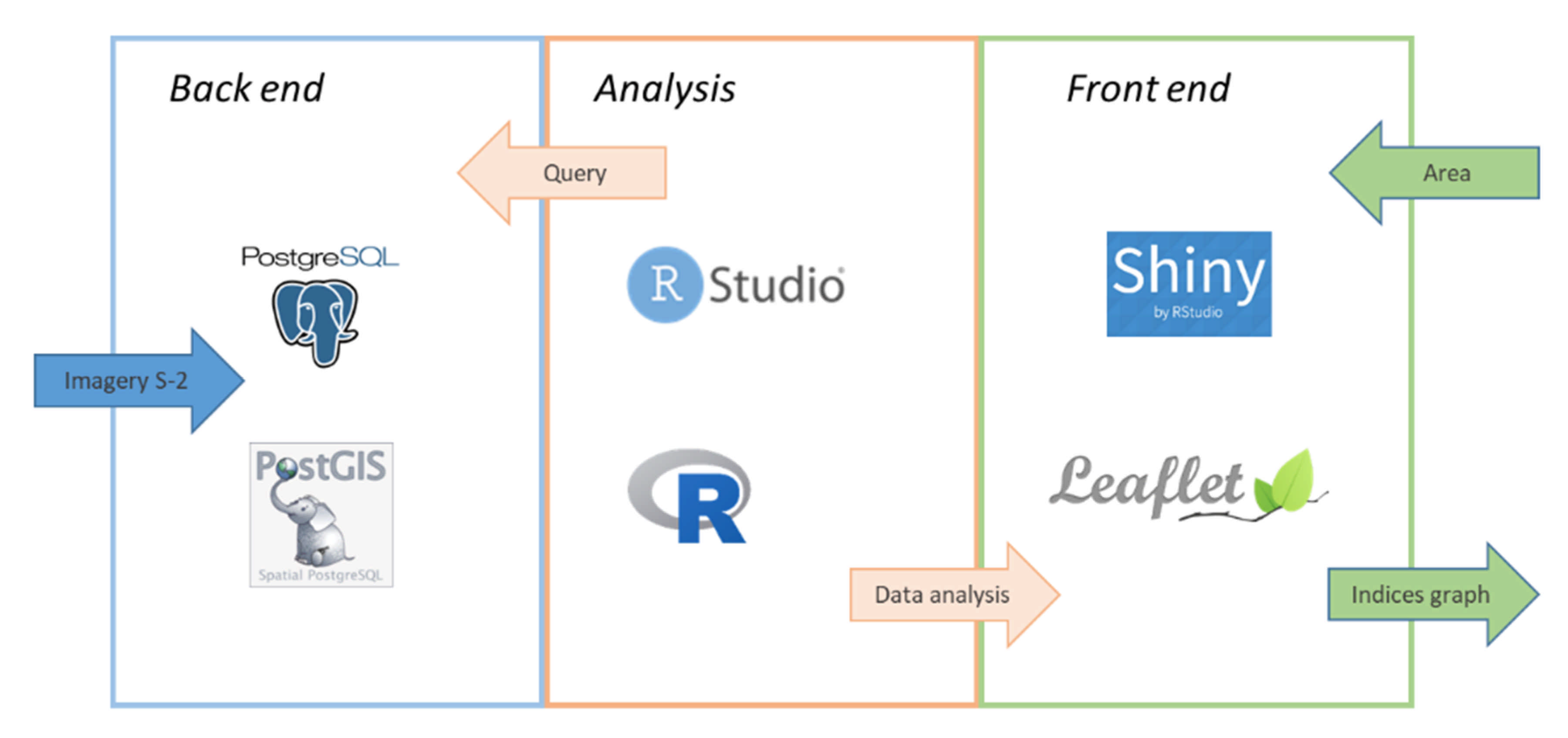
The structure of the web-GIS is composed of the back end, the analysis module, and the front end, as described in Figure 3. The satellite imagery and metadata are available through the Sentinel API Hub, so updated Level-2 images over the region of interest are automatically downloaded and stored as PostGIS elements in the PostgreSQL database. The data is kept in the original jp2 file format, and PostGIS stores meta-information (out_db option). The analysis module is based on R CRAN language, which connects the database with the front end. Therefore, the query can be launched by the user through the front-end interface that has been developed using Shiny and Leaflet packages. The user sets the parameters, which are the vegetation index, the areas drawn on the map, and the temporal window. In contrast, for the querying of the database, the threshold for the cloud coverage for each image is automatically set below 20%, and the cloud masking is automatically applied. The results are a colour-coded index map and a time-series plot (see Appendix A).
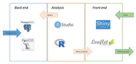
Figure 3.
Schema of the web-based platform for real-time remote sensing analysis.
3. Results and Discussion
This section is composed of three parts: (i) the temporal profile of each VI, (ii) the weight of each VI in a prediction model using machine learning, and (iii) the integration in the web-GIS portal.
3.1. Temporal Analysis
The results of the field survey and the analysis are reported in Table 1 and Table 2. Table 1 shows the names of the surveyed areas, with values of estimated severity, percent of post-event canopy cover and understorey with respective average and standard deviation of VI value in post-event imagery (September 2019). The field survey highlighted that some areas have a similar severity of damage, but different understorey, such as VOA_02, LCL_04, TA_02 and TA_01. The severity in VOA_02 is 80% and understorey cover is 70, whereas the severity in LCL_04 is 80% and understorey cover is 35%. TA_02 and TA_01 have 60% of severity and understorey cover, respectively, of 40% and 10%. Table 1 also shows the values of the VIs in September 2019. The photosynthesis rate in the Alpine regions is higher in September, i.e., tree growth. Understorey affects NDVI value in the areas with similar severity. VOA_02 and TA_02 are examples of high NDVI (~0.7) and high understorey cover in contrast with LCL_04 and TA_01. The last three rows represent control areas nearby, which were healthy stands not affected by wind damage.

Table 2.
The Spearman’s rank correlation between severity and VI average values for each month using R package, clearly showing the difference between pre-event values and post-event values of NDVI, as the storm occurred at the end of October 2018.
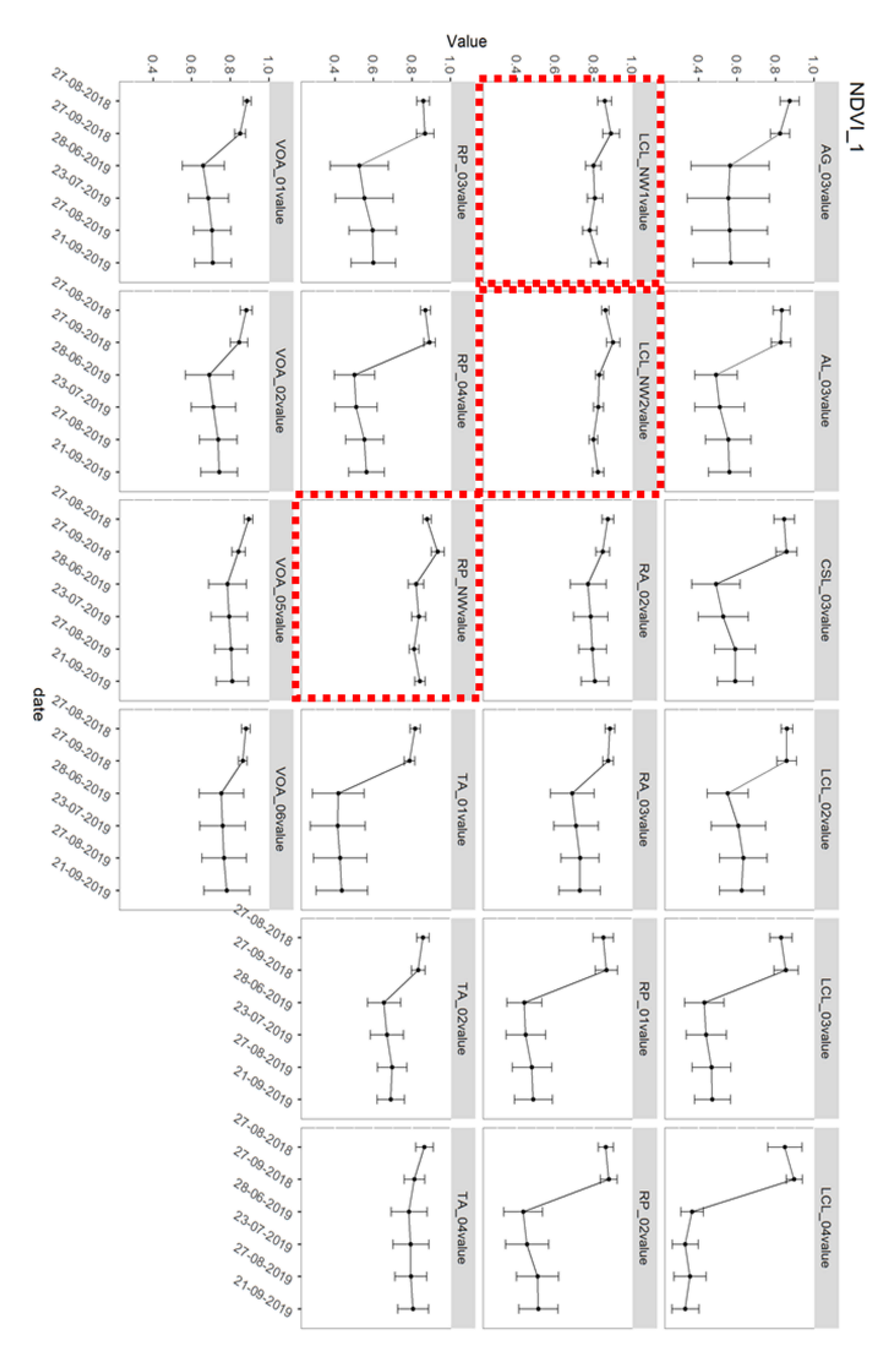
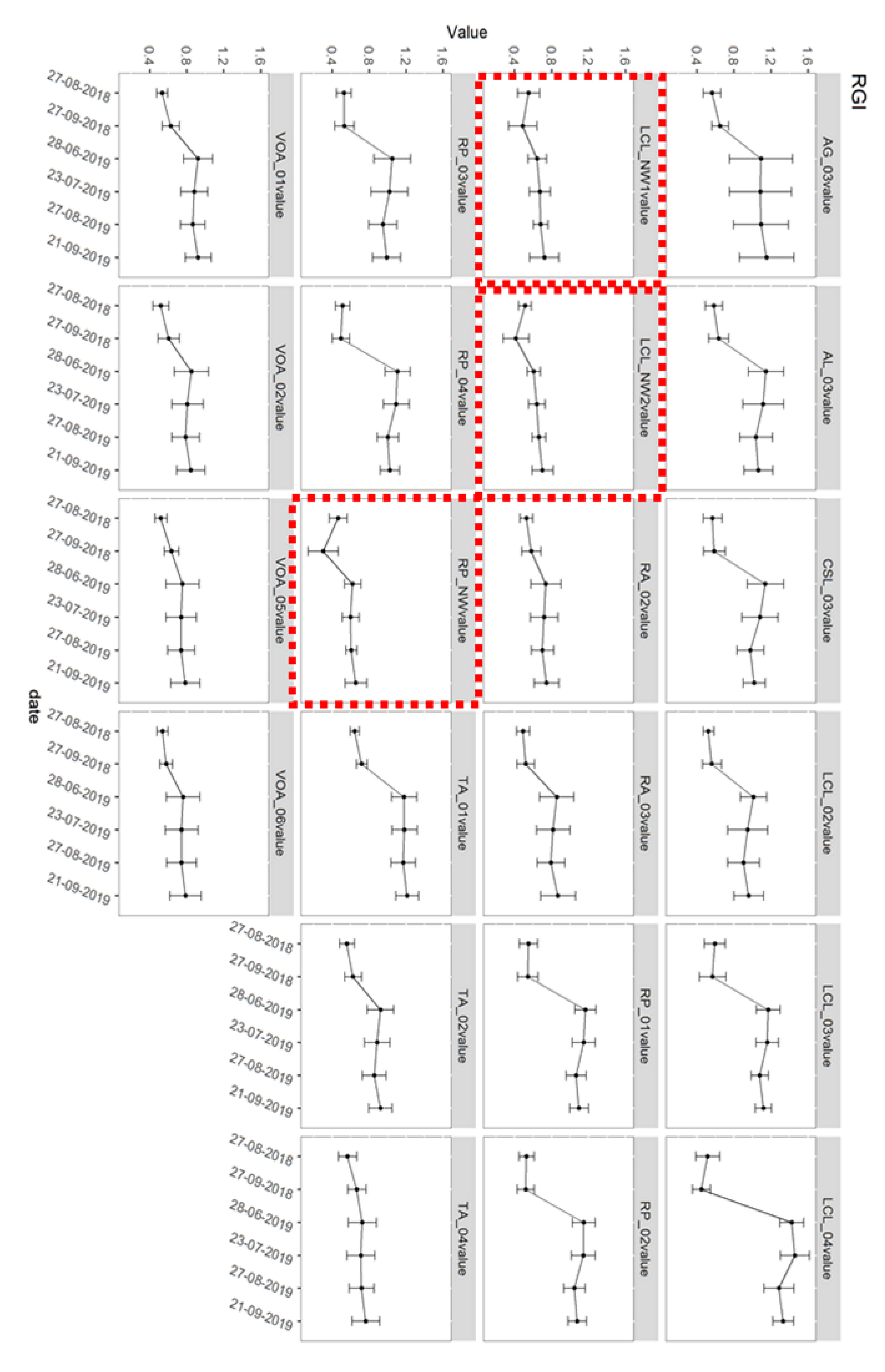
The NDVI temporal series for each plot area are reported in Figure 4. The control areas with no damage are named LCL_NW1, LCL_NW2, RP_NW (red outline), and clearly have stable NDVI values, as expected. The NDVI values in the damaged areas decrease clearly and the standard deviation increase e.g., the areas RP_03, RP_04. It is worth noting that in some damaged areas, such as the VOA_02, the NDVI values decrease to a lesser extent than other damaged areas, and the post-event values seem stable over 2019. Again, TA_01 and TA_02 both have 60% severity, but TA_01 has 10% understorey and NDVI of 0.44, TA_02 has 70% understorey and NDVI of 0.69. LCL_04 and CLS_03 are two forestry harvest area where the trunks have been removed. The soil is covered by woodchips mixed with herbaceous recovery; NDVI values in these two cases range from 0.33 to 0.59.
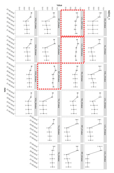
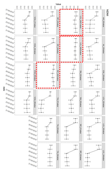
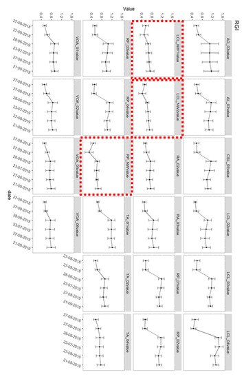
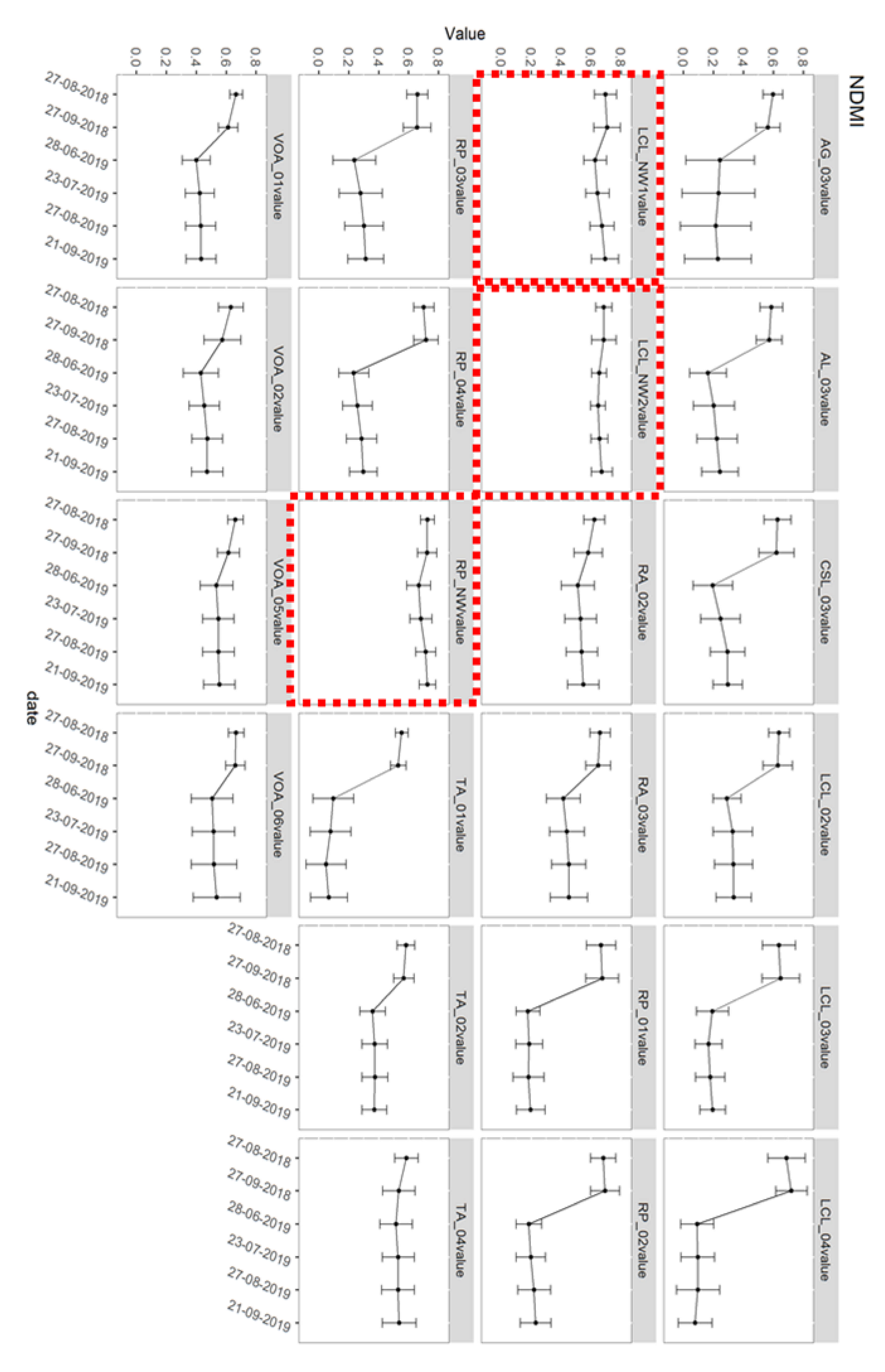
Figure 4.
Time series plot with NDVI, NDMI, and RGI average and standard deviation values. The red outline indicates the control (undamaged) areas.
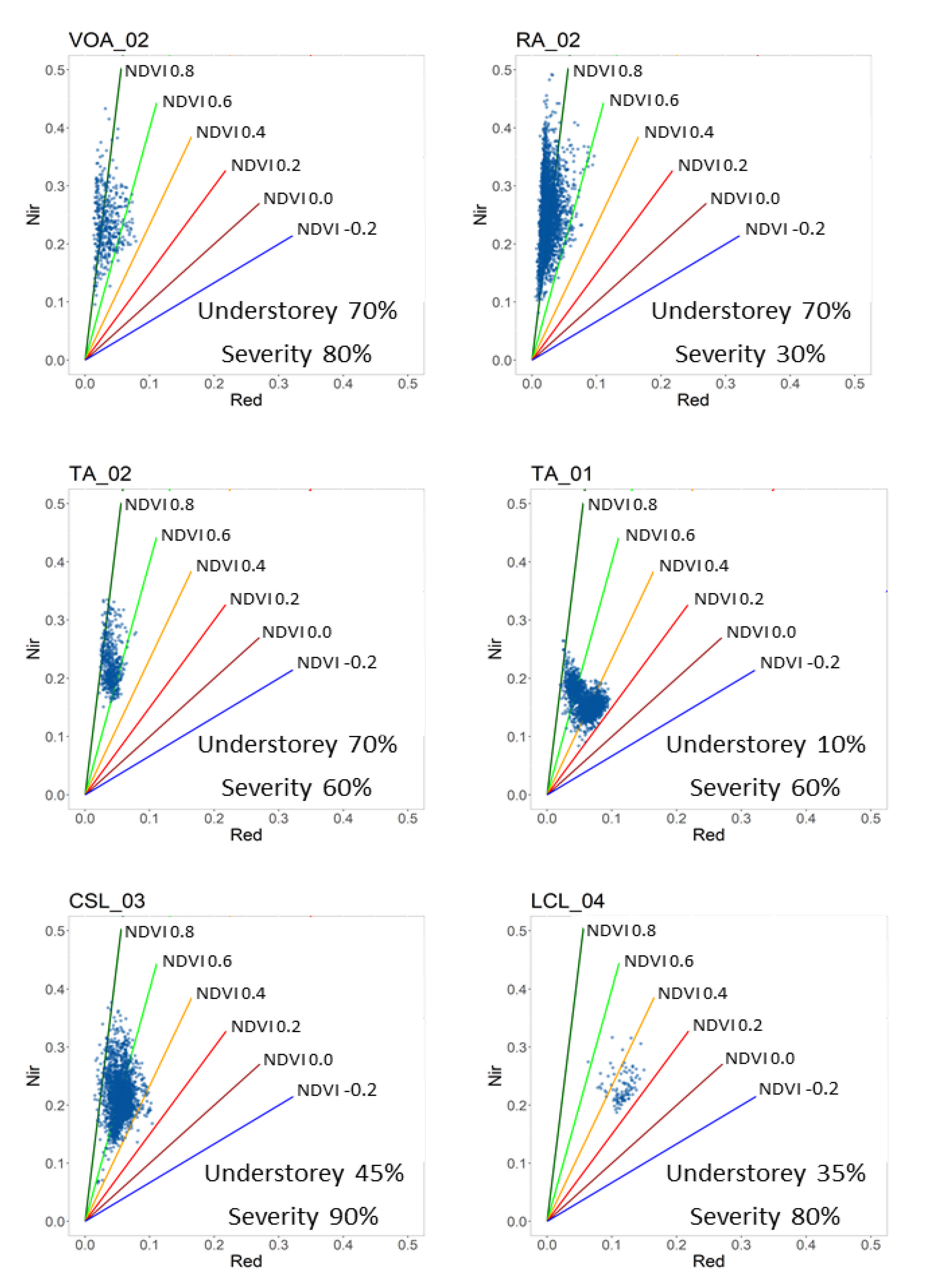
Detailed information about the effect of residual shrub cover and vegetation regeneration over NDVI at pixel scale can be observed in Figure 5. The figure shows red/nir spectral space with values of each pixel in the imagery. The points show the significant effect of post-event residual (shrub) and regenerated vegetation with the scatterplot and the NDVI baselines in September 2019. On one hand, the points of RA_02 and VOA_02 are compressed along the Y (red) axis. Both have the same shrub cover of 70%, but RA_02 site, with 30% severity, results in 0.81 value of NDVI, whereas VOA_02 has 80% severity, resulting in lower NDVI value of 0.74. In both cases, no information can be extracted about the recovery, because the NDVI value reflects vegetation that can be either from existing surviving shrub (understorey) or from recovery.
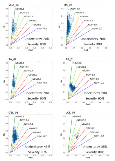
Figure 5.
Scatterplot in the red/nir spectral space: single pixel responses over the post-event imagery (September 2019). NDVI saturates when residual green cover exceeds 40%.
In contrast, in TA_02, the understorey is 70%, and the pixels’ NDVI values range between the baselines of 0.6 and 0.8. Each pixel in area TA_02 positions itself in the red/nir scatterplot, depending on the vegetation/damage fraction mixture in the pixel. Scenarios range from having a significant fraction of vegetation (0.8 NDVI value), likely due to heavy shrub or even trees resisting the storm, which cannot be differentiated in the scatterplot from regeneration. The harvesting sites show similar behavior—CLS_03 has 90% severity, but 45% of the area is recovering with herbaceous vegetation and shrubs. The points in the scatterplot in Figure 5 range between the NDVI baselines, representing 0.4 and 0.8 values. LCL_04 has 80% severity and 35% understorey, but the points in the scatterplot cover an area below the NDVI baseline 0.4. Consequently, the background reflectance of the soil can contribute to defining severity significantly when the sparse vegetation coverage (remaining shrubs or recovery) is less than 40%. Above 40% residual vegetation, the NDVI does not allow to easily distinguish a damaged area. It is worth therefore stating that it is important to record the initial post-event NDVI value, thus defining the initial per-pixel NDVI “residual” from shrubs or other resisting vegetation. Finally, a strong negative Spearman’s rank correlation between NDVI and severity was found for 2019, whereas for 2018, the correlation was not significant, as can be expected.
RGI is a simple ratio of the red and green band. In the pre-event and into the control zones, the values range between 0.65 and 0.7 (see Figure 4), which means the green reflectance is greater than the red reflectance. In the harvesting sites, the ratio becomes greater than 1, so the reflectance of red band exceeds the reflectance of the green band. In the Agordino windthrown forests, the trunks are lying on the ground since the majority of trees were uprooted. In this position, the canopy does not completely cover the trunk and the branches; therefore, the bark and soil are directly exposed and visible from the imagery. Consequently, the red spectral component increases. A strong correlation of R2 greater than 0.7 between RGI and the severity has been found (see Table 2).
NDMI has a similar trend to NDVI response, and it has a strong negative correlation with the severity. NDMI values range from 0.07 to 0.7 (see Figure 4). Healthy vegetation ranges between 0.6 and 0.8, whereas damaged areas reach a minimum of 0.2 such as RP_01. In VOA_02 that had 80% of the area damaged and the remaining understorey of 70%., average NDMI value is 0.48. Likewise, for the site RA_02, which has exactly the same understorey of 70%, the NDMI value is a bit greater, 0.55, because the severity is less than half (30%). In areas TA_01 and TA_02, both with severity of 60%, the NDMI values range between 0.07 and 0.37 due to the different remaining shrub coverage that is 10% and 40%, respectively, so the index helps to identify the fraction of bare soil and shrubs.
EVI1 and EVI2 have been tested to study the effect of the canopy fraction. Both indices have a similar trend, and they range from 0.19 to 0.52. In the pre-event, the values are quite constant around 0.5, and in the after-event, the value of the indices reach a peak at 0.6. Despite the Spearman’s correlation being negative moderate, the difference pre-post storm is not very clear, especially in the plot. These indices will not be integrated into the web application.
EWDI is calculated as the difference between the tasseled cap wetness in two sequential temporal dates. When the difference was calculated in the same year e.g., in September and August 2018, obviously no correlation with forestry damage was found. In contrast, on subtracting September 2018 to September 2019 and August 2018 to August 2019, a strong negative correlation between the index and the severity was found.
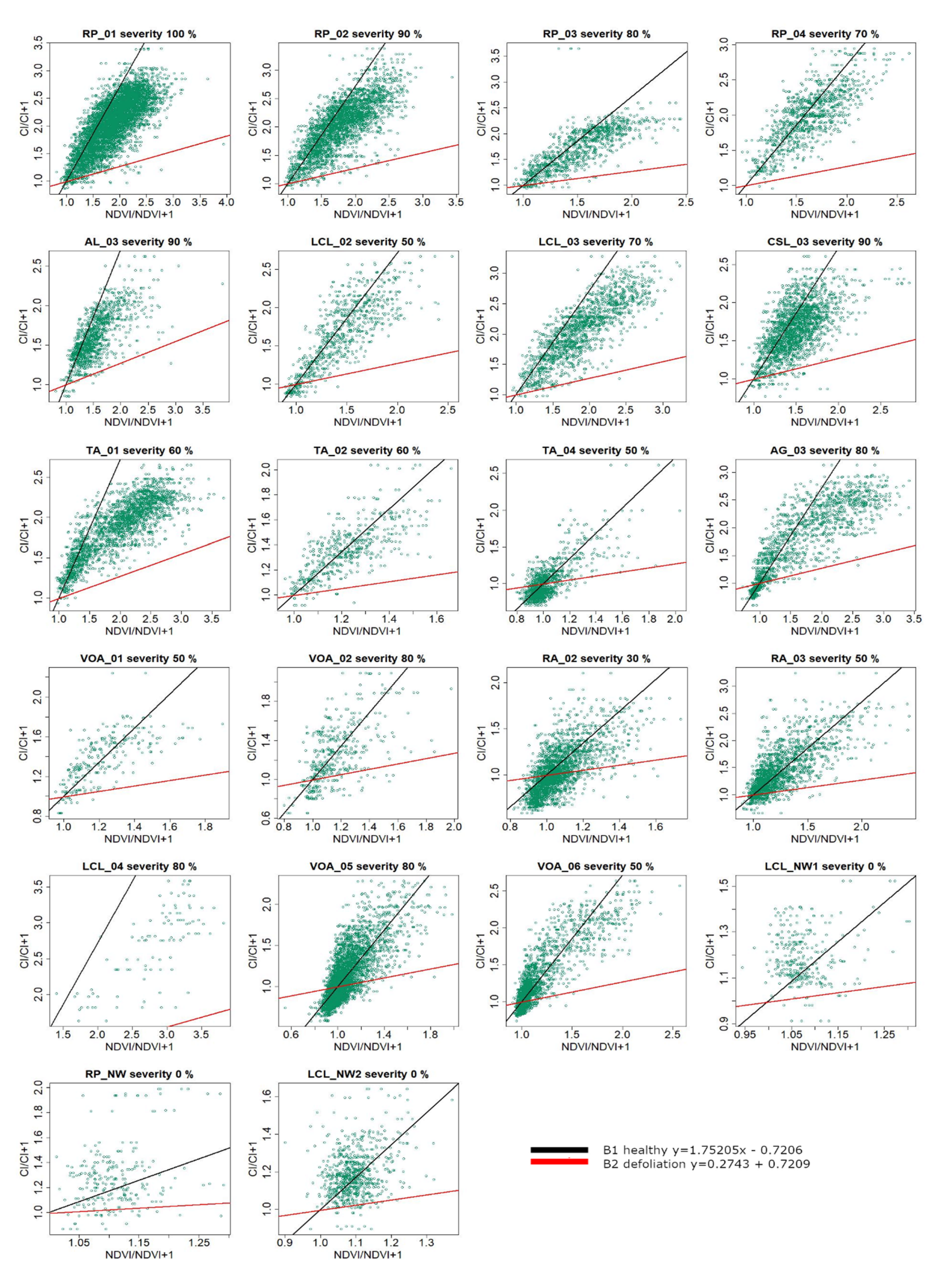
The CI index studies the response of the chlorophyll content that decreases in damaged areas. The content of chlorophyll in healthy vegetation has a value around 3 [37]. In areas with sparse green cover such as TOA_01 and TOA_02, CI ranges between 1.45 and 2.10, and the absolute minimum value from all our areas is 1.34 in LCL_04. Therefore, CI shows a strong negative correlation with the percentage of damage. The temporal variation of the CI and NDVI is reported in the scatterplots in Figure 6. In the control areas, there is no variation in chlorophyll content and NDVI response, so the scatterplot contains sparse points that do not reflect any change. In contrast, when an area is damaged, some pixels are aligned with the healthy baseline and other pixels moves from the black baseline (healthy) to the red baseline (stress), reflecting coherent results with what is reported in [37].
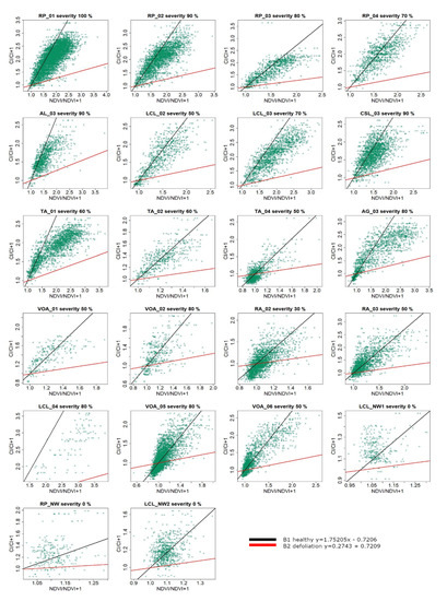
Figure 6.
The plot compares NDVI/NDVI+1 and CI/CI+1. In the area with medium and high severity, the points move from the healthy black baseline to the right. The areas with low or null severity have a compact set of points. Red and black baselines are from [37].
In conclusion, all indices except EVI1 and EVI2 can identify quite well the damaged areas. This is in line with results that report that EVIs give significant information on green biomass in non-degraded forests [43]. The visual plot of NDVI, RGI, and NDMI are easier to read and understand, and will be used for the web application. The VIs have been used for other disturbances such as bark-beetle infestation [25,33], which is a different case, but present a similar drop in photosynthetic material.
3.2. Machine Learning Analysis
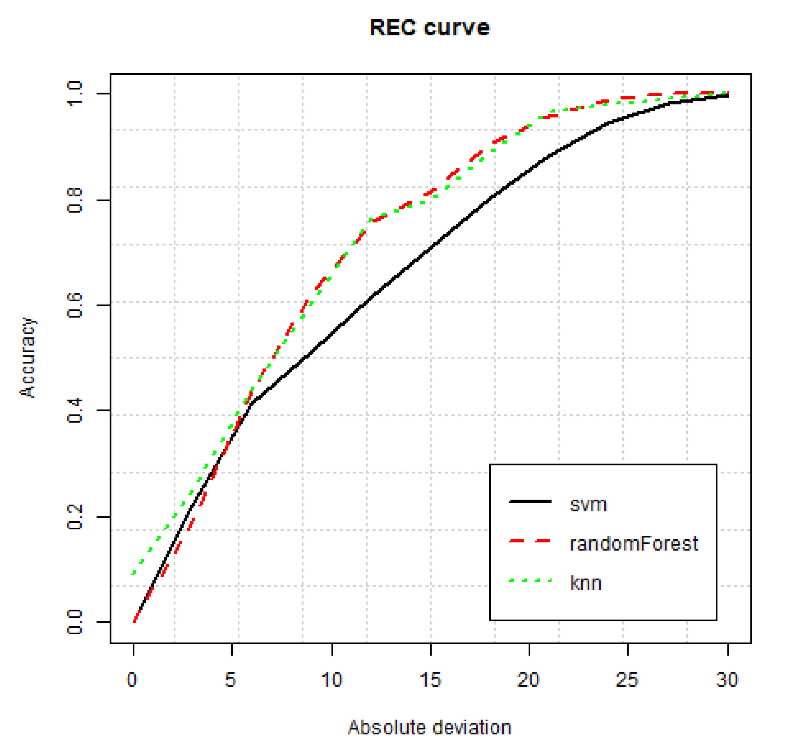
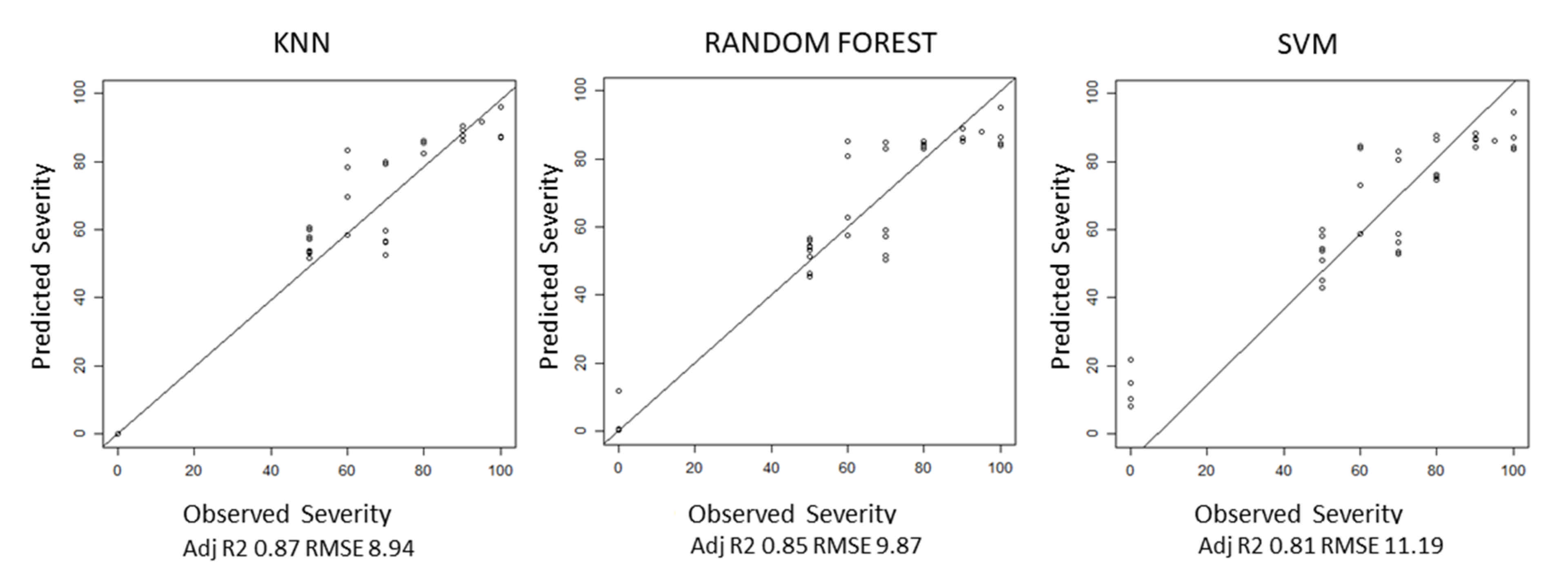
Regression with machine learning can be used to predict severity. The model parameters were tuned automatically using the Rminer package and a number of search equal to 10. Results were assessed using k-fold cross-validation, with k = 10. The regression error characteristic curve (REC), which describes the accuracy of the models, shows very similar results comparing RF, KNN, and SVM (Figure 7) with the former two having slightly better results. The differences between the first two algorithms are the importance of input variables. The most important input in both cases is NDMI, but RF takes advantage of EVI2 information to a greater degree. In contrast, KNN considers RGI as an important variable (Figure 8).
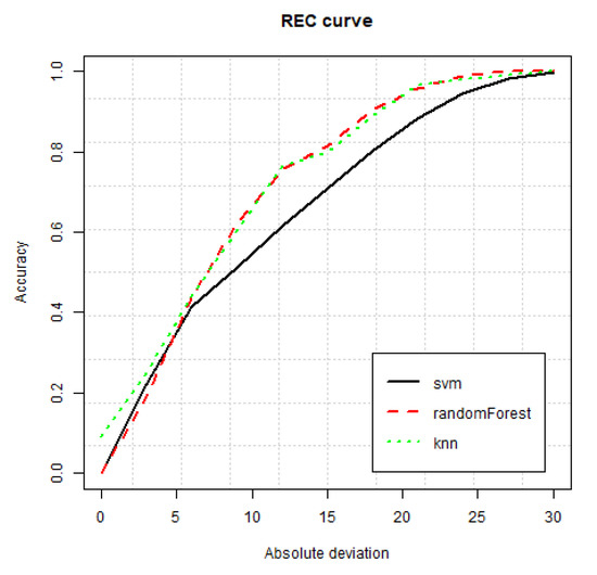
Figure 7.
REC of machine learning algorithms over predicting severity.
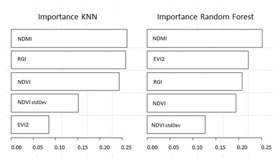
Figure 8.
Importance of indices used as a variable in machine learning for predicting severity using KNN (left) and RF (right). RF uses the information of EVI2 for the training.
The severity was then predicted using KNN, RF, SVM algorithms, and a combination of indices over the testing (Figure 9). Results for the RF algorithm, calculated using the Rminer package, are reported in Table 3. NDMI is among the better predictors in our study for severity. It must be noted that NDMI is used in the literature for detecting water stress that can be caused by abiotic or biotic factors, e.g., water availability and pathogen attacks, respectively, and damaged trees reflect a similar spectral signature. It is therefore important to use NDMI when the causality can be identified specifically.
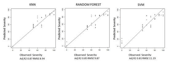
Figure 9.
Severity predicted using KNN, RF, and SVM and a combination of indices over the testing set.

Table 3.
VIs that have been used as descriptors in machine learning for predicting severity degree and have been evaluated using metrics.
The index performing less well is EVI2 with a minimum of 0.38 of adjusted R2. The NDVI has a average adjusted R2 value of 0.66, but the value increases using NDVI together with the standard deviation of NDVI; in this case the adjusted R2 reach 0.84.
4. Conclusions
The goal of this investigation is to test the potential of VIs that have proven useful in previous applications, i.e., NDVI, EVI, RGI, EWDI, NDMI, CI vs. NDVI for their potential to predict severity of forest areas damaged by windthrow in an alpine environment. The practical application of these results is to find the most suitable VIs for integrating their use in a web-GIS application, which automates the typical basic tasks in remote sensing. Remote sensing analysis requires a piece of specific knowledge and the application aims to simplify the remote sensing workflow as a support to public administration and stakeholder, which are not experts in remote sensing. The architecture is based on the PostgreSQL database and cloud computing, and allows easy and fast on-demand analysis. The analysis focuses on windthrow damage and forestry recovery. Furthermore, the indices take into consideration disturbances that can occur in the future, such as parasite attack. Studying the damaged areas using Sentinel-2 imagery, the results show a strong correlation of NDVI, RGI, and NDMI. NDVI and NDMI decrease in the damaged areas, and they have a strong negative correlation. RGI has a trend in contrast with the NDVI, and it highlights the red component of the image, such as bark, branches, and soil. It is a simple ratio, easy to calculate using a red green blue (RGB) camera, which is the base equipment of commercial drones. If detailed inspection is necessary, UAVs imagery can integrate satellite analysis [35]. NDMI has a behaviour similar to NDVI, but it is specific for water stress. Finally, the plots in Figure 4 summarize the temporal behavior of the VIs at the sites. The control areas have a stable trend in 2018 and 2019 and the damaged areas show a variation in the index with an increase in standard deviation. Hence, damaged areas can be recognized, but green coverage greater than 40% influences the indices’ response. Above this percentage, the apparent forest recovery can be due to shrubs, herbs, or regenerating trees, so field survey is required. KNN and RF assign different importance to the VI. KNN uses NDMI, RGI, and NVI whereas RF focus on NDVI, EVI2, and RGI. RF gives less importance to NDVI than KNN. However, severity prediction using RF produced good results using NDMI or NDVI and the NDVI standard deviation. In this study, the surveyed areas describe the various case histories in terms of exposure, slope, and severity in the Agordino area. However, further analysis is necessary for integrating Sentinel-1 and Sentinel-2, or applying the model to other Alpine or Pre-Alpine areas affected by the Vaia storm. After two years from the storm, more investigation can focus on disturbances due to parasites near damaged areas, such as to study forest health by applying machine learning.
Future work is expected, both related to the analytical part and to the web-GIS. Regarding the analytical part, tests will be done adding Sentinel-1 information, which might provide added and non-collinear information with respect to the optical information from Sentinel-2. In addition, the regeneration will be monitored with the VIs that have been assessed, to see the sensibility of such information to recovery of the vegetation in the area. The web-GIS will continue development, to provide automated visualization and analysis of Sentinel-2 data online. In particular, it is planned to add specific per-pixel cloud probability that can be calculated with more accurate methods (e.g., s2cloudless [44]) in order to have a finer definition of reliable pixel values. Users will also be able to define their own threshold for cloud probability.
Author Contributions
Investigation, C.Z. & M.P.; formal analysis and software, M.P.; writing—original draft preparation, M.P. & C.Z.; writing, revision, validation, supervision, and editing, F.P.; validation and revision, E.L.; supervision, funding and revision S.G. All authors have read and agreed to the published version of the manuscript.
Funding
This research was funded by the Unione Montana Agordina and the University of Padova under the framework of the InForTrac project (UNI-IMPRESA 2018) and by TESAF Department, University of Padova, in the framework of the project “Vaia FRONT” (CAVA_SID19_02).
Institutional Review Board Statement
Not applicable.
Informed Consent Statement
Not applicable.
Data Availability Statement
Data available on request due to restrictions.
Acknowledgments
The authors acknowledge the support of the Unione Montana Agordina.
Conflicts of Interest
The authors declare no conflict of interest.
Appendix A
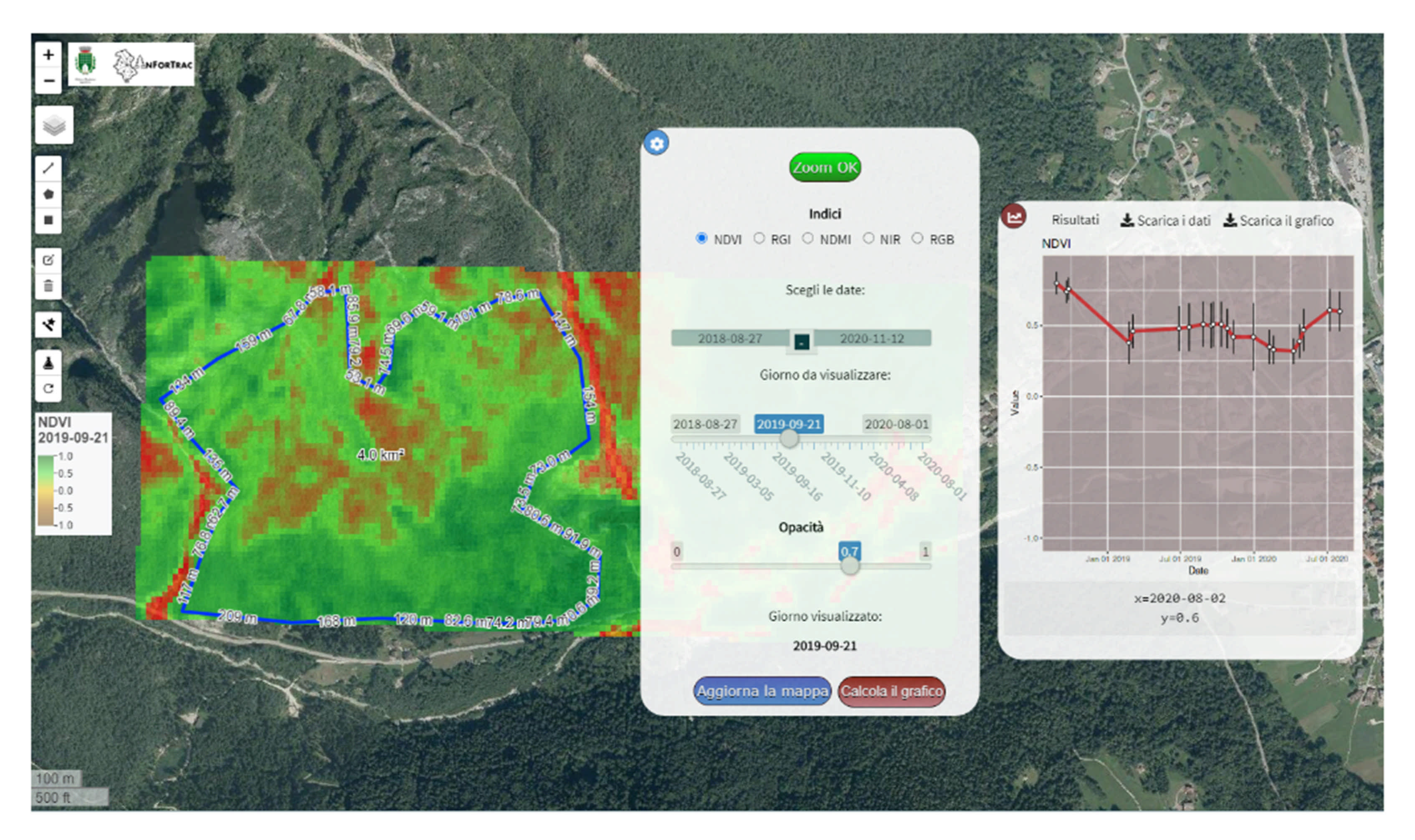
The investigation led to identifying better VIs for monitoring forest damage that can be successively deployed in the web application. The web application aims to help forestry technicians and public administrations and stakeholders in forest planning and management. In the current stage, the software integrates three indices, determined using previous investigation on correlation and variable importance using machine learning regression. The indices used are NDVI, RGI, and NDMI. Figure A1 shows an example of the interface. On the left, a toolbar allows to select the layer displayed, to activate a measuring tool and to draw a polygon where the VI analysis will be done. Then, VI and the temporal domain are chosen in the setting panel. All available Sentinel-2 images, which spatially overlap the testing area, are clipped and masked. Masking consists of removing pixels which belong to “cloud (high probability)”, “cloud (medium probability)”, and “cloud-shadow” in the “Scene Classification” (SCL) product of the Level 2C Sentinel-2 product. Masking is an important step, which removes gross errors in the time-series data that are created by the user in real-time and might be used for further processing.
A downloadable zonal statistic plot with average and standard deviation of the selected VI is produced. The color-scaled index map is automatically displayed, and the time bar allows to change the VI images that are created on-the-fly and projected in the map. The following items provide an overview of the service provided by the web platform to end-users:
- draws, over the view area, a styled raster of the chosen VI, automatically clipping and masking;
- creates a downloadable zonal statistic plot reporting average and standard deviation values of pixels inside the selected area for all images in the temporal scale;
- provides a downloadable report with raw values with id, timestamp, average, and standard deviation calculated from all images over the user-selected area (the data used for creating the plot described in the previous point).
Available Sentinel-2 Level-2C images are automatically downloaded through a script that checks for available new images each day. This is done only over one specific tile, (TQS32) as the project had a specific study area to be investigated.

Figure A1.
The web application consists of three elements: the toolbar (on the left), the setting panel, and the result panel (on the right).
Figure A1.
The web application consists of three elements: the toolbar (on the left), the setting panel, and the result panel (on the right).
Appendix B

Table A1.
Sev. = Severity (in %); Avg. = Average, Std. = Standard deviation.
Table A1.
Sev. = Severity (in %); Avg. = Average, Std. = Standard deviation.
| 21/09/2019 | Sev. | Canopy | Under- | NDVI | RGI | NDMI | |||
|---|---|---|---|---|---|---|---|---|---|
| Cover | Storey | Avg. | Std. | Avg. | Std. | Avg. | Std. | ||
| RP_01 | 100 | 5 | 5 | 0.486 | 0.099 | 1.098 | 0.103 | 0.197 | 0.096 |
| CSL_03 | 90 | 0 | 45 | 0.591 | 0.092 | 1.02 | 0.120 | 0.295 | 0.098 |
| AL_03 | 90 | 5 | 40 | 0.561 | 0.109 | 1.064 | 0.157 | 0.242 | 0.122 |
| RP_02 | 90 | 10 | 10 | 0.513 | 0.101 | 1.077 | 0.102 | 0.23 | 0.103 |
| VOA_02 | 80 | 30 | 70 | 0.742 | 0.095 | 0.843 | 0.153 | 0.473 | 0.105 |
| VOA_05 | 80 | 60 | 40 | 0.810 | 0.084 | 0.784 | 0.156 | 0.554 | 0.104 |
| LCL_04 | 80 | 5 | 35 | 0.332 | 0.071 | 1.333 | 0.112 | 0.078 | 0.114 |
| AG_03 | 80 | 0 | 15 | 0.569 | 0.197 | 1.153 | 0.295 | 0.229 | 0.224 |
| RP_03 | 80 | 5 | 15 | 0.599 | 0.115 | 0.989 | 0.150 | 0.313 | 0.120 |
| RP_04 | 70 | 20 | 25 | 0.565 | 0.093 | 1.024 | 0.104 | 0.297 | 0.093 |
| LCL_03 | 70 | 10 | 10 | 0.472 | 0.093 | 1.119 | 0.088 | 0.194 | 0.085 |
| TA_02 | 60 | 40 | 70 | 0.690 | 0.071 | 0.923 | 0.124 | 0.371 | 0.084 |
| TA_01 | 60 | 10 | 10 | 0.436 | 0.133 | 1.210 | 0.122 | 0.068 | 0.124 |
| VOA_06 | 50 | 60 | 60 | 0.782 | 0.119 | 0.787 | 0.171 | 0.536 | 0.156 |
| TA_04 | 50 | 60 | 50 | 0.806 | 0.081 | 0.762 | 0.149 | 0.537 | 0.114 |
| VOA_01 | 50 | 30 | 50 | 0.710 | 0.095 | 0.924 | 0.139 | 0.432 | 0.101 |
| RA_03 | 50 | 60 | 40 | 0.727 | 0.108 | 0.870 | 0.188 | 0.452 | 0.124 |
| LCL_02 | 50 | 25 | 25 | 0.625 | 0.116 | 0.960 | 0.160 | 0.336 | 0.117 |
| RA_02 | 30 | 30 | 70 | 0.805 | 0.071 | 0.745 | 0.133 | 0.548 | 0.104 |
| LCL_NW1 | 0 | - | - | 0.829 | 0.043 | 0.721 | 0.157 | 0.693 | 0.092 |
| LCL_NW2 | 0 | - | - | 0.822 | 0.029 | 0.701 | 0.114 | 0.672 | 0.071 |
| RP_NW | 0 | - | - | 0.841 | 0.028 | 0.657 | 0.118 | 0.726 | 0.055 |
| 21/09/2019 | Sev. | Canopy | Under- | EVI1 | EVI2 | CI | |||
| Cover | Storey | Avg. | Std. | Avg. | Std. | Avg. | Std. | ||
| RP_01 | 100 | 5 | 5 | 0.233 | 0.071 | 0.228 | 0.068 | 1.575 | 0.237 |
| CSL_03 | 90 | 0 | 45 | 0.317 | 0.081 | 0.310 | 0.079 | 1.880 | 0.246 |
| AL_03 | 90 | 5 | 40 | 0.298 | 0.087 | 0.293 | 0.083 | 1.785 | 0.295 |
| RP_02 | 90 | 10 | 10 | 0.256 | 0.070 | 0.249 | 0.068 | 1.662 | 0.248 |
| VOA_02 | 80 | 30 | 70 | 0.420 | 0.108 | 0.405 | 0.103 | 2.544 | 0.434 |
| VOA_05 | 80 | 60 | 40 | 0.457 | 0.114 | 0.441 | 0.107 | 3.022 | 0.567 |
| LCL_04 | 80 | 5 | 35 | 0.192 | 0.056 | 0.197 | 0.053 | 1.338 | 0.181 |
| AG_03 | 80 | 0 | 15 | 0.316 | 0.160 | 0.316 | 0.152 | 1.967 | 0.714 |
| RP_03 | 80 | 5 | 15 | 0.309 | 0.089 | 0.301 | 0.087 | 1.898 | 0.363 |
| RP_04 | 70 | 20 | 25 | 0.328 | 0.089 | 0.318 | 0.086 | 1.812 | 0.276 |
| LCL_03 | 70 | 10 | 10 | 0.234 | 0.054 | 0.228 | 0.052 | 1.572 | 0.219 |
| TA_02 | 60 | 40 | 70 | 0.370 | 0.080 | 0.361 | 0.077 | 2.099 | 0.209 |
| TA_01 | 60 | 10 | 10 | 0.186 | 0.068 | 0.184 | 0.066 | 1.457 | 0.279 |
| VOA_06 | 50 | 60 | 60 | 0.383 | 0.115 | 0.370 | 0.109 | 2.786 | 0.625 |
| TA_04 | 50 | 60 | 50 | 0.522 | 0.156 | 0.504 | 0.147 | 2.927 | 0.497 |
| VOA_01 | 50 | 30 | 50 | 0.376 | 0.089 | 0.364 | 0.085 | 2.386 | 0.386 |
| RA_03 | 50 | 60 | 40 | 0.384 | 0.110 | 0.373 | 0.104 | 2.464 | 0.471 |
| LCL_02 | 50 | 25 | 25 | 0.346 | 0.109 | 0.337 | 0.105 | 1.992 | 0.367 |
| RA_02 | 30 | 30 | 70 | 0.475 | 0.125 | 0.457 | 0.117 | 3.053 | 0.508 |
| LCL_NW1 | 0 | - | - | 0.342 | 0.092 | 0.334 | 0.088 | 2.978 | 0.314 |
| LCL_NW2 | 0 | - | - | 0.451 | 0.135 | 0.446 | 0.135 | 2.922 | 0.193 |
| RP_NW | 0 | - | - | 0.454 | 0.106 | 0.445 | 0.101 | 3.108 | 0.232 |
| 21/09/2019 | Sev. | Canopy | Under- | EDWI Sep. 19-18 | EDWI Aug. 19-18 | EDWI 2018 | |||
| Cover | Storey | Avg. | Std. | Avg. | Std. | Avg. | Std. | ||
| RP_01 | 100 | 5 | 5 | −0.043 | 0.015 | −0.047 | 0.018 | 0.006 | 0.007 |
| CSL_03 | 90 | 0 | 45 | −0.046 | 0.025 | −0.049 | 0.027 | 0.007 | 0.010 |
| AL_03 | 90 | 5 | 40 | −0.048 | 0.022 | −0.053 | 0.024 | 0.006 | 0.008 |
| RP_02 | 90 | 10 | 10 | −0.041 | 0.018 | −0.045 | 0.020 | 0.006 | 0.007 |
| VOA_02 | 80 | 30 | 70 | −0.030 | 0.025 | −0.028 | 0.025 | 0.011 | 0.014 |
| VOA_05 | 80 | 60 | 40 | −0.017 | 0.018 | −0.014 | 0.020 | 0.011 | 0.009 |
| LCL_04 | 80 | 5 | 35 | −0.080 | 0.026 | −0.079 | 0.035 | 0.006 | 0.013 |
| AG_03 | 80 | 0 | 15 | −0.043 | 0.034 | −0.045 | 0.039 | 0.009 | 0.011 |
| RP_03 | 80 | 5 | 15 | −0.039 | 0.019 | −0.042 | 0.020 | 0.006 | 0.009 |
| RP_04 | 70 | 20 | 25 | −0.048 | 0.020 | −0.047 | 0.021 | 0.006 | 0.010 |
| LCL_03 | 70 | 10 | 10 | −0.043 | 0.018 | −0.049 | 0.021 | 0.006 | 0.008 |
| TA_02 | 60 | 40 | 70 | −0.038 | 0.017 | −0.036 | 0.018 | 0.010 | 0.008 |
| TA_01 | 60 | 10 | 10 | −0.044 | 0.011 | −0.048 | 0.013 | 0.007 | 0.004 |
| VOA_06 | 50 | 60 | 60 | −0.017 | 0.018 | −0.015 | 0.021 | 0.009 | 0.009 |
| TA_04 | 50 | 60 | 50 | −0.017 | 0.024 | −0.015 | 0.025 | 0.009 | 0.016 |
| VOA_01 | 50 | 30 | 50 | −0.028 | 0.016 | −0.026 | 0.016 | 0.009 | 0.009 |
| RA_03 | 50 | 60 | 40 | −0.030 | 0.023 | −0.024 | 0.023 | 0.012 | 0.011 |
| LCL_02 | 50 | 25 | 25 | −0.033 | 0.020 | −0.036 | 0.024 | 0.008 | 0.010 |
| RA_02 | 30 | 30 | 70 | −0.021 | 0.025 | −0.014 | 0.025 | 0.013 | 0.013 |
| LCL_NW1 | 0 | - | - | −0.004 | 0.012 | 0.001 | 0.014 | 0.005 | 0.011 |
| LCL_NW2 | 0 | - | - | −0.002 | 0.016 | −0.001 | 0.013 | 0.000 | 0.018 |
| RP_NW | 0 | - | - | −0.004 | 0.016 | 0.001 | 0.015 | 0.003 | 0.016 |
References
- Mantero, G.; Morresi, D.; Marzano, R.; Motta, R.; Mladenoff, D.J.; Garbarino, M. The Influence of Land Abandonment on Forest Disturbance Regimes: A Global Review. Landsc. Ecol. 2020, 35, 2723–2744. [Google Scholar] [CrossRef]
- Albrich, K.; Rammer, W.; Seidl, R. Climate Change Causes Critical Transitions and Irreversible Alterations of Mountain Forests. Glob. Chang. Biol. 2020, 26, 4013–4027. [Google Scholar] [CrossRef] [PubMed]
- Beniston, M. Climatic Change in Mountain Regions: A Review of Possible Impacts. In Climate Variability and Change in High Elevation Regions: Past, Present & Future. Advances in Global Change Research; Diaz, H.F., Ed.; Springer: Dordrecht, The Netherlands, 2003; Volume 15. [Google Scholar]
- Schelhaas, M.-J.; Nabuurs, G.-J.; Schuck, A. Natural Disturbances in the European Forests in the 19th and 20th Centuries. Glob. Chang. Biol. 2003, 9, 1620–1633. [Google Scholar] [CrossRef]
- Schelhaas, M.-J.; Hengeveld, G.; Moriondo, M.; Reinds, G.J.; Kundzewicz, Z.W.; ter Maat, H.; Bindi, M. Assessing Risk and Adaptation Options to Fires and Windstorms in European Forestry. Mitig. Adapt. Strat. Glob. Chang. 2010, 15, 681–701. [Google Scholar] [CrossRef]
- Shikhov, A.N.; Perminova, E.S.; Perminov, S.I. Satellite-Based Analysis of the Spatial Patterns of Fire- and Storm-Related Forest Disturbances in the Ural Region, Russia. Nat. Hazards 2019, 97, 283–308. [Google Scholar] [CrossRef]
- Gregow, H.; Laaksonen, A.; Alper, M.E. Increasing Large Scale Windstorm Damage in Western, Central and Northern European forests, 1951–2010. Sci. Rep. 2017, 7, 46397. [Google Scholar] [CrossRef]
- Usbeck, T.; Wohlgemuth, T.; Dobbertin, M.; Pfister, C.; Bürgi, A.; Rebetez, M. Increasing Storm Damage to Forests in Switzerland from 1858 to 2007. Agric. Meteorol. 2010, 150, 47–55. [Google Scholar] [CrossRef]
- Brůna, J.; Wild, J.; Svoboda, M.; Heurich, M.; Müllerová, J. Impacts and Underlying Factors of Landscape-Scale, Historical Disturbance of Mountain Forest Identified Using Archival Documents. Ecol. Manag. 2013, 305, 294–306. [Google Scholar] [CrossRef]
- Gardiner, B.; Blennow, K.; Carnus, J.-M.; Fleischer, P.; Ingemarson, F.; Landmann, G.; Lindner, M.; Marzano, M.; Nicoll, B.; Orazio, C.; et al. Destructive Storms in European Forests: Past and Forthcoming Impacts. Final Report to European Commission-DG Environment; European Forest Institute: Joensuu, Finland, 2010. [Google Scholar]
- Biolchi, S.; Denamiel, C.; Devoto, S.; Korbar, T.; Macovaz, V.; Scicchitano, G.; Vilibić, I.; Furlani, S. Impact of the October 2018 Storm Vaia on Coastal Boulders in the Northern Adriatic Sea. Water (Switzerland) 2019, 11, 2229. [Google Scholar] [CrossRef]
- Chirici, G.; Giannetti, F.; Travaglini, D.; Nocentini, S.; Francini, S.; D’Amico, G.; Calvo, E.; Fasolini, D.; Broll, M.; Maistrelli, F.; et al. Forest Damage Inventory After the “Vaia” Storm in Italy. Riv. Selvic. Ed. Ecol. 2019, 16, 3–9. [Google Scholar] [CrossRef]
- Forzieri, G.; Pecchi, M.; Girardello, M.; Mauri, A.; Klaus, M.; Nikolov, C.; Rüetschi, M.; Gardiner, B.; Tomaštík, J.; Small, D.; et al. A Spatially Explicit Database of Wind Disturbances in European Forests over the Period 2000–2018. Earth Syst. Sci. Data 2020, 12, 257–276. [Google Scholar] [CrossRef]
- Virot, E.; Ponomarenko, A.; Dehandschoewercker, É.; Quéré, D.; Clanet, C. Critical Wind Speed at Which Trees Break. Phys. Rev. E 2016, 93, 023001. [Google Scholar] [CrossRef]
- Copernicus Emergency Management Service Mapping. Available online: https://emergency.copernicus.eu/mapping/list-of-components/EMSR334 (accessed on 18 January 2021).
- Bolyn, C.; Michez, A.; Gaucher, P.; Lejeune, P.; Bonnet, S. Forest Mapping and Species Composition Using Supervised per Pixel Classification of Sentinel-2 Imagery. Biotechnol. Agron. Soc. Environ. 2018, 22, 16. [Google Scholar]
- Poursanidis, D.; Chrysoulakis, N. Remote Sensing, Natural Hazards and the Contribution of ESA Sentinels Missions. Remote Sens. Appl. Soc. Environ. 2017, 6, 25–38. [Google Scholar] [CrossRef]
- Gorelick, N.; Hancher, M.; Dixon, M.; Ilyushchenko, S.; Thau, D.; Moore, R. Google Earth Engine: Planetary-scale Geospatial Analysis for Everyone. Remote Sens. Environ. 2017, 202, 18–27. [Google Scholar] [CrossRef]
- Vaglio Laurin, G.; Francini, S.; Luti, T.; Chirici, G.; Pirotti, F.; Papale, D. Satellite Open Data to Monitor Forest Damage Caused by Extreme Climate-Induced Events: A Case Study of the Vaia Storm in Northern Italy. Int. J. Res. 2020. [Google Scholar] [CrossRef]
- Huete, A.; Justice, C.; Van Leeuwen, W. MODIS Vegetation Index (MOD13); The University of Arizona: Tucson, AZ, USA, 1999; Volume 3. [Google Scholar]
- Verbesselt, J.; Hyndman, R.; Newnham, G.; Culvenor, D. Detecting Trend and Seasonal Changes In Satellite Image Time Series. Remote Sens. Environ. 2010, 114, 106–115. [Google Scholar] [CrossRef]
- Bausch, W.C. Soil Background Effects on Reflectance-Based Crop Coefficients for Corn. Remote Sens. Envrion. 1993, 46, 213–222. [Google Scholar] [CrossRef]
- Huete, A.R.; Liu, H.Q.; van Leeuwen, W.J.D. Use of Vegetation Indices in Forested Regions: Issues of Linearity and Saturation. Int. Geosci. Remote Sens. Symp. 1997, 4, 1966–1968. [Google Scholar]
- Huete, A.R. A Soil-Adjusted Vegetation Index (SAVI). Remote Sens. Environ. 1988, 25, 295–309. [Google Scholar] [CrossRef]
- Hall, R.J.; Castilla, G.; White, J.C.; Cooke, B.J.; Skakun, R.S. Remote Sensing of Forest Pest Damage: A Review and Lessons Learned from a Canadian Perspective. Can. Entomol. 2016, 148, S296–S356. [Google Scholar] [CrossRef]
- Rullan-Silva, C.D.; Olthoff, A.E.; Delgado de la Mata, J.A.; Pajares-Alonso, J.A. Remote Monitoring of Forest Insect Defoliation. A review. For. Syst. 2013, 22, 377–391. [Google Scholar] [CrossRef]
- Abdullah, H.; Skidmore, A.K.; Darvishzadeh, R.; Heurich, M. Sentinel-2 Accurately Maps Green-Attack Stage of European Spruce Bark Beetle (Ips typographus, L.) Compared with Landsat-8. Remote Sens. Ecol. Conserv. 2019, 5, 87–106. [Google Scholar] [CrossRef]
- Hart, S.J.; Veblen, T.T. Detection of Spruce Beetle-Induced Tree Mortality using High- and Medium-Resolution Remotely Sensed Imagery. Remote Sens. Environ. 2015, 168, 134. [Google Scholar] [CrossRef]
- Coops, N.C.; Johnson, M.; Wulder, M.A.; White, J.C. Assessment of Quickbird High Spatial Resolution Imagery to Detect Red Attack Damage Due to Mountain Pine Beetle Infestation. Remote Sens. Environ. 2006, 103, 67–80. [Google Scholar] [CrossRef]
- Wulder, M.A.; White, J.C.; Bentz, B.; Alvarez, M.F.; Coops, N.C. Estimating the Probability of Mountain Pine Beetle Red-Attack Damage. Remote Sens. Environ. 2006, 101, 150–166. [Google Scholar] [CrossRef]
- Wulder, M.A.; White, J.C.; Coops, N.C.; Butson, C.R. Multi-Temporal Analysis of High Spatial Resolution Imagery for Disturbance Monitoring. Remote Sens. Environ. 2008, 112, 2729–2740. [Google Scholar] [CrossRef]
- Gamon, J.A.; SurfurusS, J.S. Assessing leaf pigment content and activity with a reflectometer. New Phytol. 1999, 143, 105–117. [Google Scholar] [CrossRef]
- Coops, N.C.; Waring, R.H.; Wulder, M.A.; White, J.C. Prediction and Assessment of Bark Beetle-Induced Mortality of Lodgepole Pine Using Estimates Of Stand Vigor Derived From Remotely Sensed Data. Remote Sens. Environ. 2009, 113, 1058–1066. [Google Scholar] [CrossRef]
- Crist, E.P.; Cicone, R.C. Comparisons of the Dimensionality and Features of Simulated Landsat-4 MSS and TM data. Remote Sens. Environ. 1984, 14, 235–246. [Google Scholar] [CrossRef]
- Goodwin, N.R.; Coops, N.C.; Wulder, M.A.; Gillanders, S.; Schroeder, T.A.; Nelson, T. Estimation of Insect Infestation Dynamics Using a Temporal Sequence of Landsat Data. Remote Sens. Environ. 2008, 112, 3680–3689. [Google Scholar] [CrossRef]
- Wilson, E.H.; Sader, S.A. Detection of Forest Harvest Type using Multiple Dates of Landsat TM Imagery. Remote Sens. Environ. 2002, 80, 385–396. [Google Scholar] [CrossRef]
- Zarco-Tejada, P.J.; Hornero, A.; Hernández-Clemente, R.; Beck, P.S.A. Understanding the Temporal Dimension of the Red-Edge Spectral Region for Forest Decline Detection using High-Resolution Hyperspectral and Sentinel-2a Imagery. Isprs J. Photogramm. Remote Sens. 2018, 137, 134–148. [Google Scholar] [CrossRef]
- Main-Knorn, M.; Pflug, B.; Louis, J.; Debaecker, V.; Müller-Wilm, U.; Gascon, F. Sen2Cor for Sentinel-2. In Proceedings of the Image and Signal Processing for Remote Sensing XXIII; Bruzzone, L., Bovolo, F., Benediktsson, J.A., Eds.; SPIE: Bellingham, WA, USA, 2017; p. 3. [Google Scholar]
- Cortes, C.; Vapnik, V. Support-Vector Networks. Mach. Learn. 1995, 20, 273–297. [Google Scholar] [CrossRef]
- Shi, T.; Horvath, S. Unsupervised Learning With Random Forest Predictors. J. Comput. Graph. Stat. 2006, 15, 118–138. [Google Scholar] [CrossRef]
- Cortez, P. Data Mining with Neural Networks and Support Vector Machines Using the R/rminer Tool. In Advances in Data Mining. Applications and Theoretical Aspects. ICDM 2010. Lecture Notes in Computer Science; Springer: Berlin/Heidelberg, Germany, 2010; Volume 6171, pp. 572–583. ISBN 978-3-642-14399-1. [Google Scholar]
- Cortez, P.; Embrechts, M.J. Using Sensitivity Analysis and Visualization Techniques to Open Black Box Data Mining Models. Inf. Sci. (N. Y.) 2013, 225, 1–17. [Google Scholar] [CrossRef]
- Eckert, S. Improved Forest Biomass and Carbon Estimations Using Texture Measures from WorldView-2 Satellite Data. Remote Sens. 2012, 4, 810–829. [Google Scholar] [CrossRef]
- Sanchez, A.H.; Picoli, M.C.A.; Camara, G.; Andrade, P.R.; Chaves, M.E.D.; Lechler, S.; Soares, A.R.; Marujo, R.F.B.; Simões, R.E.O.; Ferreira, K.R.; et al. Comparison of Cloud Cover Detection Algorithms on Sentinel-2 Images of the Amazon Tropical Forest. Remote Sens. 2020, 12, 1284. [Google Scholar] [CrossRef]
Publisher’s Note: MDPI stays neutral with regard to jurisdictional claims in published maps and institutional affiliations. |
© 2021 by the authors. Licensee MDPI, Basel, Switzerland. This article is an open access article distributed under the terms and conditions of the Creative Commons Attribution (CC BY) license (https://creativecommons.org/licenses/by/4.0/).


