Abstract
Point cloud registration is one of the basic research hotspots in the field of 3D reconstruction. Although many previous studies have made great progress, the registration of rock point clouds remains an ongoing challenge, due to the complex surface, arbitrary shape, and high resolution of rock masses. To overcome these challenges, a novel registration method for rock point clouds, based on local invariants, is proposed in this paper. First, to handle the massive point clouds, a point of interest filtering method based on a sum vector is adopted to reduce the number of points. Second, the remaining points of interest are divided into several cluster point sets and the centroid of each cluster is calculated. Then, we determine the correspondence between the original point cloud and the target point cloud by proving the inherent similarity (using the trace of the covariance matrix) of the remaining point sets. Finally, the rotation matrix and translation vector are calculated, according to the corresponding centroids, and a correction method is used to adjust the positions of the centroids. To illustrate the superiority of our method, in terms of accuracy and efficiency, we conducted experiments on multiple datasets. The experimental results show that the method has higher accuracy (about ten times) and efficiency than similar existing methods.
1. Introduction
With the continuous advancement of laser scanning technology, the use of laser scanners as tools to generate 3D point clouds of complex scenes for structural engineering applications has been greatly promoted. However, due to technical limitations, when scanning large scenes, single-site scanning usually only obtains partial angle data of the scene and cannot obtain complete scene data. In addition, when affected by object occlusion, even small scenes require multi-station scanning coverage of the whole scene [1]. Therefore, to obtain complete scene data, the fusion of multi-station scanning data is one of the fundamental and important approaches in the field of 3D point cloud research.
However, several characteristics of rock mass point clouds jointly hinder the application of existing methods. First, these point clouds are usually massive. Generally, rock mass data collection in the field environment is larger than collection in urban or indoor environments. Tens of millions of points can be collected in one scan, which makes algorithms with high time complexity impractical. Second, the associated resolution is high. The resolution of terrestrial laser scanners has reached the millimeter level, allowing for the preservation of details and accurate surface information. However, a disadvantage of registration is that this high resolution makes it difficult to extract unique features from a single point, as it is difficult to identify features that distinguish a point from nearby similar points, which means that points with similar features will be clustered. When a point does not have sufficient discriminating ability, the corresponding point matched in the two scans will be unreliable. Third, the surface of a rock mass is complex and irregular. Unlike objects in urban or indoor scenes, the surface of the rock mass is highly different.
This article mainly focuses on the point clouds of rock masses, due to the characteristics of rock masses described above. In addition, it is difficult to extract features from natural vegetation and defined regions of interest in a wide range of flat areas (e.g., plains and deserts), which makes it necessary to consider the problem from a holistic perspective. The local sharp features (i.e., interesting registration points) are more obvious for rock mass.
Based on the above considerations, we propose a new registration method, which is mainly divided into the following steps: First, to efficiently and accurately extract the above feature area points, a new interesting point detection method, called sum vector filtration (), is proposed. counts the sum vector formed by a center point and its neighbors, which measures the amount of change between each point p and its neighbors . In this way, the interesting points (Section 3.1) of the rock mass point cloud are selected, in order to reduce the amount of data. Then, the remaining points are clustered and the point cloud rotation invariant is calculated, in order to determine the corresponding relationship. Finally, centroid correction is applied to obtain more accurate registration results. Our main contributions are made in addressing the following problems: (1) efficiently handling massive data; (2) fully utilizing high-resolution data; and (3) extracting robust features from irregular surfaces.
The remainder of this paper is organized as follows. Section 2 provides a quick review of other algorithms related to this work. Section 3 presents the entire framework and implementation details of the proposed method. Section 4 reports the experimental results and analysis. Section 5 discusses the highlights, possible extensions, and limitations of our work.
2. Related Work
Generally speaking, point cloud registration methods can be divided into two categories: coarse registration and fine registration [2]. The purpose of coarse registration is to estimate the initial transformation between the initial point cloud and the target point cloud. The resulting calibration is usually further refined using the iterative closest point (ICP) algorithm [3] or its variants [4,5,6,7,8]. There are two reasons that demonstrate the importance of the coarse registration and fine registration processes for point cloud registration: First, the ICP algorithm starts from an initial estimate of the rigid body transformation. If the two point clouds are not close in space, the ICP algorithm may fall into a local minimum. Secondly, the ICP algorithm requires a good initial transformation to improve the computational efficiency of the algorithm, especially when processing high-resolution data.
2.1. Coarse Registration
Coarse registration methods can be divided into two categories: sampling point methods [9,10,11,12,13,14] and feature-based methods. According to the selected features, feature-based methods can be further subdivided into three categories: local feature-based methods [15,16,17,18], global feature-based methods [2,19,20,21,22,23], and depth feature-based methods [24,25,26,27,28].
Sampling point methods: These methods select a number of points in the target point cloud and the original point cloud, either randomly or according to specific rules, and then compare the selected points to find the corresponding relationship.
Chen et al. [9] proposed a registration method based on random sampling consistency. It first randomly selects three non-collinear points from the original point cloud, and a triangle can be constructed from the three points selected. Similarly, the method finds three points in the target point cloud that are similar to the triangle formed by the three points randomly selected from the original point cloud. Assuming that the three pairs of non-collinear points have a corresponding relationship, a rotation matrix and translation vector can be obtained by the three pairs of corresponding points. Repeating the above operation k times, k rotation matrices and translation vectors are calculated, and, finally, through comparison, the rotation matrix and translation vector with the smallest registration error are selected as the final result. This method has strong robustness, but it is obvious that the method needs to find all points in the target point cloud that have a corresponding relationship with the filtered points in the original point cloud, which causes the method to have lower computational efficiency.
Different from randomly selecting non-collinear points, Aiger et al. [10] proposed a registration method based on the use of four coplanar points (4PCS), which reduces spatial matching operations by constructing and matching congruent four-point pairs, thereby accelerating the registration process. Specifically, their method constructs a coplanar four-point set in the original point cloud P and the target point cloud Q of any pose, using affine invariance constraints, matching the corresponding point pairs that meet the conditions in the coplanar four-point set. The largest common pointset (LCP) strategy is used to find the four-point pairs with the largest overlap after registration, thus obtaining the optimal matching result. Based on the 4PCS method, many improved methods have been proposed. For example, the Super-4PCS [11] algorithm adopts an intelligent indexing strategy to reduce the computational complexity of the 4PCS algorithm. In K-4PCS [12], sparse key points are used to replace the random sampling points of the original algorithm, in order to achieve high-precision point cloud registration. The Generalized 4PCS [13] and Super Generalized 4PCS [14] algorithms improve the construction process for the original algorithm with four coplanar points, generalize the construction of the coplanar four-point base, and no longer strictly restrict the four points to co-exist on a plane.
Feature-based methods: Feature-based methods usually involve similar processes, including feature extraction, description, and matching. The extracted features mainly include local, global, and depth features. The following describes feature-based registration methods, according to the different features used.
(1) Local feature-based methods Generally, the local feature-based coarse registration method first filters some feature points through use of a point cloud filtering method, mainly including Gaussian curvature [15], feature lines, planes, and other features. Then, feature descriptors are constructed for the remaining feature points, and the original and target point clouds are matched through the correspondence of feature descriptors.
Rusu et al. [16] proposed the use of point feature histograms (PFH) to encode the shape information of local surfaces, which has a strong discriminating ability but is extremely time-consuming. To solve this problem, Rusu et al. [17] later used a simplified point feature histogram (SPFH) to construct a fast point feature histogram (FPFH), which has the characteristics of fast and strong discriminating ability; however, the normal quality of the point cloud has a great influence on the FPFH. Tombari et al. [18] proposed the signature of histograms of orientations (SHOT) method. SHOT first divides the local sphere into subspaces, then calculates a normal vector and key point normal deviation for each subspace, thus reflecting the points in the subspace, and finally calculates the concatenation vector of each subspace corresponding feature. Although SHOT is very descriptive, it is sensitive to changes in point density resolution. Wang et al. [15] used the Gaussian curvature to filter registration points of interest, established a complete graph of N-sections to find the correspondence, and used Singular Value Decomposition (SVD) to decompose the conversion matrix, in order to obtain a more ideal registration effect.
(2) Global feature-based methods Unlike local features, which only focus on neighboring points, global features reflect higher-level geometric features. The main global features include lines and surfaces. Habib et al. [19] and Al-Durgham et al. [20] proposed registration frameworks based on straight lines, but their methods require the data to have obvious straight line characteristics. Based on this, Yang and Zang [21] extended the straight line to a curve, which reduced the algorithm’s dependence on the data but, at the same time, increased the algorithm complexity. Different from the line-based method, the surface-based method has higher robustness. Hu et al. [2] proposed a method based on plane polygon matching. Their method first extracts a plane from the data and then uses principal component analysis to project the polygons surrounding the plane into the same space and calculates the overlap ratio to determine the correspondence between the planes. However, this method requires a number of common planes in the overlap area. Dold et al. [22] proposed a registration method that uses corresponding image information to optimize plane matching. V4PCS [23] improves the efficiency of the algorithm by establishing a voxel-based four-face congruence set. Registration methods based on global features are more robust to noise and point cloud density changes than methods based on local features; however, these methods have higher requirements, in terms of the data used, and require the data to have obvious line and surface features.
(3) Depth feature-based methods With the rapid development of deep learning networks, some methods using deep learning features to represent manual design features have emerged. Differing from other registration methods, this type of method searches for corresponding relationships at the feature level. Zeng et al. [24] proposed to realize the corresponding 3DMatch between local three-dimensional data by learning the descriptors of local spatial blocks. Their method finds the closest key points in the 3DMatch descriptor space by calculating the 3DMatch descriptor. Gojcic [25] proposed a framework of 3DSmoothNet, which uses the Siamese network to learn feature representations with smaller local point clouds. Wang et al. [26] proposed an end-to-end method, which first uses the network to learn point cloud features, and then introduces an attention mechanism for approximate matching operations. There also exist some registration algorithms that integrate multiple methods, such as Aoki [27], which combines pointnet [28] point cloud feature learning methods with traditional Lucas and Kanade (LK) image registration methods [29]. These methods have obtained good results on some data, but require a pre-trained network, which means that these methods require a large amount of training data and have poor scalability.
2.2. Fine Registration
Fine registration mainly refers to ICP [3] and its derived algorithms [4,6,8,30,31,32,33,34,35]. The ICP algorithm is one of the most widely used 3D point cloud registration algorithms. It uses a Euclidean transformation approach to solve the rotation and translation matrix of two point clouds and the corresponding registration error. The ICP algorithm continuously solves the estimated transformation matrix, until the root mean square error (RMSE) registration error converges to the local optimal solution. Although ICP has the advantages of simplicity and good convergence, it is limited by the initial position of the point cloud and can easily fall into a local optimal solution when solving the point cloud registration problem with outliers.
To improve the robustness of the ICP algorithm, scholars have proposed a series of variants of the ICP algorithm. The LM-ICP [30] algorithm uses the Levenberg–Marquardt algorithm to solve the ICP registration model. It use the Distance–Transform (DT) algorithm to replace the KD-tree for searching for the nearest neighbors, thus reducing the influence of the initial position of the point cloud on the registration results and improve the registration efficiency. On the basis of the ICP algorithm, a more robust and practical Trimmed ICP [31] algorithm has been proposed. In this method, the nearest neighbors obtained from each iteration are selected; that is, the Euclidean distances of the matched points, estimated in pairs, are sorted and discarded. For the point set with a larger distance, the penalty percentage is dynamically calculated by the kernel function. When the Trimmed ICP algorithm is applied to the point cloud registration problem with outliers and noise, it can obtain good registration accuracy. However, the high proportion of outliers still poses a huge challenge to the robustness requirements of the point cloud registration algorithm. Bouaziz et al. proposed the Sparse ICP [6] algorithm, which uses sparse representation theory to further improve the robustness of the ICP algorithm, i.e. increasing the p-norm penalty term in the norm registration model to improve the accuracy of solving matching points in each iteration. However, the use of an augmented Lagrangian to solve large-scale point cloud registration problems is inefficient. Mavridis et al. [32] proposed a more efficient Sparse ICP algorithm, combined with the simulated annealing algorithm, to accelerate the convergence speed of point cloud registration.
Under the premise of obtaining a better initial position of the point cloud, the iterative nearest point algorithm has good robustness in solving the point cloud registration problem; however, there are also some shortcomings that can continue to be optimized, such as the slow convergence as the number of iterations increases and the high time cost of searching for the nearest neighbor. In response to the above shortcomings, scholars have differed from the iterative closest point registration algorithm to construct new registration models, such as probability density models, implicit least squares functions, Gaussian mixture models, and combinations of other optimization algorithms, in order to improve the point cloud registration efficiency and precision. Magnusson et al. [36] proposed the normal distribution transform (NDT) algorithm based on the probability density model, which uses the D-dimensional Gaussian function as the registration model. Whether the corresponding point cloud is divided into the same voxel is an important factor affecting the final result of the method. The biggest advantage of the algorithm is that the nearest neighbor matching point does not need to be solved during the iteration process; as such, it has low computational complexity. Gruen and Akca [37] proposed a method that estimates the transformation parameters between 3D surface patches through minimizing the Euclidean distances between corresponding surfaces by least squares. Matching is achieved by minimizing a goal function. As the functional model for least squares matching is non-linear, initial approximations for the parameters must be provided. Jian et al. [38] proposed the use of a mixed Gaussian model to replace a single Gaussian model. To improve the robustness of the registration model, the voxel Gaussian model is weighted separately, such as NDT, EM-ICP [4], and so on. Aiming at the accuracy of point cloud registration, some scholars have proposed point-to-plane [33], point-to-line [34], surface-to-surface [35], and generalized iterative closest point (G-ICP) [8] methods. However, these methods still suffer from sensitivity to the initial position. Pomerleau et al. [39] conducted comparative experiments on the variant ICP method using real data and pointed out the advantages and disadvantages of various methods.
In summary, whether a registration method is based on local features or global features, it depends on the feature description. In addition, some methods build descriptors based on all points, which are inefficient when faced with massive rock mass point clouds. Compared with traditional registration methods, methods based on depth features have obtained excellent results on certain datasets; however, these results all rely on a trained model, which makes these methods lack scalability, in general, and they usually require a large amount of pre-training of the model using labeled data. The ICP algorithm and most of its variant methods still have the shortcomings of being sensitive to the initial position of the point cloud and can easily to fall into a local optimum. The iterative finding of corresponding points between the source point cloud and the target point cloud reduces the efficiency of the algorithm.
Inspired by the methods mentioned above, we propose an efficient registration solution for rock mass point clouds. In the proposed method, we use the invariances of point of interest sets, in terms of rotation and translation, to perform a coarse registration, then fine-tune the centroids to achieve fine registration. This avoids a heavy computational burden while achieving high accuracy.
3. Methodology
This section details the key steps of the proposed registration method, including filtering points of interest, clustering, pair matching, and centroid correction (see Figure 1).
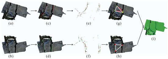
Figure 1.
The main stages of the proposed method: (a,b) the input target point cloud and source point cloud, respectively; (c,d) the filtered points of interest, represented as red points in (c) and green points in (d); (e,f) the cluster results and centroids, represented as green points in (e) and red points in (f); (g,h) examples illustrating the centroid correction step (the yellow point in the target point cloud is the feature point location after correction); and (i) the registration result. The green color explains that the image in (i) is the result of registration, which is different from the one in (a).
3.1. Filtering Points of Interest
Generally, an ideal feature point should exist in a salient area that is different from surrounding regions and describes the most important and distinctive information content. Therefore, as shown in Figure 2, four types of areas in the rock mass are considered characteristic areas:
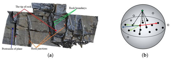
Figure 2.
(a) Locations of four types of points of interest. Red indicates corner points, green indicates the protruding parts of the rock boundary, orange indicates the rock junctions, and blue indicates a plane protrusion. (b) A point of interest (green) and a non-interest point (red).
- (1)
- The tip of the rock: It is mainly located at the tip of the rock or a part of the rock.
- (2)
- The protruding part of the rock boundary: In general, the boundary of the rock is not a strictly straight line and, thus, the bulge of the boundary is considered to be the main feature on the rock boundary.
- (3)
- Bedding trace: The junction area of two or more rocks merges the features of multiple rocks.
- (4)
- Plane protrusion: In the rock mass, there may be protrusions in a plane area, and the characteristics of this area are obviously different from those of the surrounding plane.
The local value of a center point, p, is defined as:
where W represents the Gaussian weight function, r is the sampling radius, represents the nearest point sampling method to sample the neighborhood point , and k represents the sample number of .
In fact, as shown in Figure 2b, the points in the above four characteristic regions obtain a larger value. In other words, in a planar area, the vector formed by the center point (the red points) and one of the neighboring points (the red line in Figure 2b) will have at least one vector that is symmetrical to the center point (green lines in Figure 2b and the blue line, which is the sum vector of the two green lines), which makes the value smaller. On the contrary, the direction of the vector formed by the feature area points and its neighbors is similar and has a positive correlation with the sum vector (the green point and black lines in Figure 2b), which leads to a larger value for feature area points.
When the calculation of the value (Figure 3b) is completed, the points with values between the thresholds and are retained as points of interest (Figure 3c), where is used to delete those points with relatively small values, generally points in a flat area, and is used to eliminate some outliers (as shown in Figure 4). The retained points of interest are usually only a small part of the initial points. Such a filtering operation is considered necessary when registering a large number of rock mass point clouds. For example, as shown in Figure 3c, for a point cloud with 300,000 initial points, after the feature point filtering operation, only 3600 points of interest were retained. For clarity, the remaining points are denoted as and , which represent the target points of interest and the original points of interest, respectively.
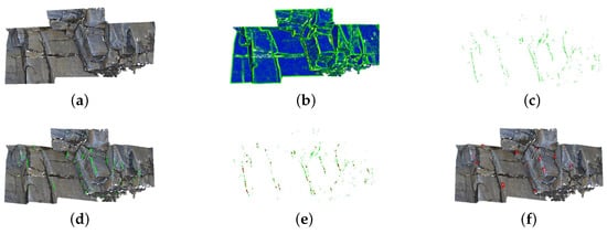
Figure 3.
Data processed in different stages of feature extraction: (a) original point cloud; (b) value distribution of the original point cloud; (c) points of interest after filtering operation; (d) points of interest in the original point cloud; (e) centroids of the clusters; and (f) centroids in the original point cloud.
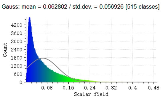
Figure 4.
The value distribution of Figure 3b.
3.2. Clustering
The preserved points of interest are distributed in various feature regions, and those in the same feature region are clustered with each other. At this stage, these points of interest are divided into several cluster centers, according to the density-based spatial clustering of applications with noise (DBSCAN) [40] algorithm. What needs to be considered in the clustering process is the clustering radius, which should not be too large or too small. On the one hand, if the clustering radius is too small, the clusters will be unstable and multiple clustering centers may be obtained in the same characteristic region. On the other hand, if the clustering radius is too large, multiple feature areas will be classified into the same category when the distance between them is relatively close. Both of the above situations will have a negative impact on the final registration. In fact, a clustering radius which is applicable to all data does not exist. To obtain valid clustering results, we considered clustering on multiple scales, and then empirically chose a reasonable scale.
By clustering, points of interest are classified into a small set of clustering points. The cluster center of each cluster point set is calculated and regarded as the feature point. The cluster center of the target point cloud and the point of interest of the source point cloud are denoted as and , respectively. As shown in Figure 3e,f, this process further reduces the number of points and obtains more representative feature points.
3.3. Pair Matching
After the above processing stages, several cluster centers and points of interest around each cluster center are retained. The purpose of this stage is to determine which correspondences exist in and . Different from constructing descriptors for each feature point and surrounding points of interest, we take each cluster point set as the research object, find that they undergo invariant amounts of translation and rotation, and judge the similarity between the clustering point sets and based on this characteristic.
Assuming that and are the ith corresponding centers in and , and the rotation matrix and translation vector between them are R and t, respectively, then can be represented by :
If and are denoted as cluster point sets corresponding to and , respectively, as the point set is composed of several points of interest, the corresponding relationship between points in and is affected by the order of the point set. To eliminate the point concentration point set , a permutation matrix X is used to adjust the order of the point concentration. Then, we use to represent , as
Let , be the mean of and , respectively, and let and denote and , respectively. Then, we obtain
where X is the permutation matrix. Assuming =1, then . Obviously, it can be obtained that, after the rotation, and have the same trace.
More generally, the method is used to sample k representative points on and , respectively, which is as follows:
Then, each cluster set has a corresponding centroid, and, finally, the obtained centroid is used to find the rotation matrix and the translation vector.
The similarity between two cluster sets can usually be judged by Formula (6) at multiple scales. However, there may be some mismatched point sets in complex scenes. To solve this problem, we select the first as corresponding point sets, and then select corresponding point sets for verification. For example, the first three most similar corresponding point sets may be considered to be the correct matching point set pairs, after which several remaining point set pairs can be randomly selected for verification. If a smaller mean square error is obtained, the selected corresponding point set pair is considered to be a correct matching set.
3.4. Centroid Correction
Although each clustering point set can get their accurate clustering center through calculation, the corresponding clustering center is biased, due to various aspects (e.g., noise and missing points). At this stage, a cluster center position correction method is used to adjust the position of cluster centers. As shown in Figure 5, the cluster centers , and the cluster centers , are the corresponding feature points located in the target point cloud and the original point cloud, respectively. When the feature point in the target point cloud is known, the corresponding feature point, , in the original cloud can be expressed as
where k is the size of , represents the Euclidean distance between and p, ℓ is the search error threshold, and is the th set of clustering points after correction.
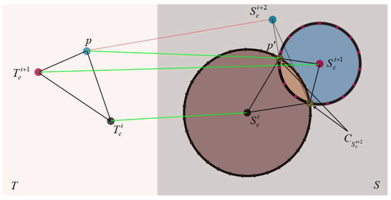
Figure 5.
Illustration of centroid correction process. On the left, the centroids of the target point cloud are shown. is the original location of the centroid corresponding to p, while is the corrected location.
In fact, when a pair of feature points are known, the position of the second pair of feature points can be corrected accordingly. When two pairs of feature points are known, only a small number of candidate positions are left. Similarly, if three pairs of feature points are known, the position of the fourth pair of feature points will be locked to a few areas. If more corresponding feature points are known, the remaining feature points can be calculated theoretically.
4. Experimental Results and Analysis
The proposed registration method was implemented based on the PCL (Point Cloud Library) [41] library, which includes: point cloud pre-processing, Kd-tree establishment, SVD decomposition for the transformation matrix, ICP registration, and point cloud visualization. The code was executed on an Intel (R) Core i7-4790 3.60 GHz CPU with 4.00 GB RAM.
To verify the effectiveness and efficiency of the proposed registration method, the following comparative experimental methods were used:
- -
- The NDT method, proposed by Magnusson et al. [36], solves the transformation matrix based on statistical information after voxelizing the point cloud, which was provided with the PCL library.
- -
- The Generalized-ICP (G-ICP), proposed by Segal et al. [8], optimizes the distance criterion of the traditional ICP algorithm, which was provided with the PCL library.
- -
- The Plane Detection and Polygon Matching (PPB) method, proposed by Hu et al. [2], establishes the corresponding relationship, according to the proportion of the plane polygon area of the overlapping part, which was executed using the code provided by Hu et al. [2].
- -
- The N-point Complete Graphs (NCG) method, proposed by Wang et al. [15], uses the Gaussian curvature to select feature points (points of interest) and N-point complete graphs to calculate the transformation matrix, which was executed using the code provided by Wang et al. [15].
In this section, the parameters, test data, and evaluation metrics are introduced. Finally, the registration results of our method and the comparison method for rock mass point clouds are used for comparison and analysis.
4.1. Parameter Tuning
Table 1 lists the main parameters used in the proposed method. As shown in Table 1, these parameters were divided into four groups.

Table 1.
Summary of the parameters.
In the point of interest filtering stage, the parameters of r, , and were used to calculate the SVF value. Among them, r was used to determine the range of the local point cloud for calculating the SVF value, and were used to limit the range of the SVF value, and the points with SVF values between and were retained. When the number of collected points is larger and the search radius is larger, and can be increased appropriately. k is the number of sampling points, which was used to uniformly participate in the calculation of the SVF value. is the threshold for selecting valid clusters, and cluster sets with less than points were deleted. The optimal settings of k and are proportional to the point cloud density. In the clustering stage, is the clustering threshold, which was used to determine which cluster set the unknown point of interest belongs to. is the minimum number of points allowed in the valid clusters, and clusters with fewer than points were considered invalid clusters. Similarly, is the maximum distance allowed by a legal cluster, and, when the farthest point in a cluster was further than , it was considered an invalid cluster. When the point cloud density is larger, theoretically, and should also increase. In the pair matching stage, is the maximum difference for judging the similarity of two point sets. When the difference is greater than , it was considered that there was no correspondence between the two point sets. is the number of sampling points, and its function was similar to that of k. In centroid correction stage, l was used to correct the error threshold of the feature point position. is similar to and k, being the number of sampling points in this stage. In the pair matching and centroid correction stages, the setting of these parameters was based on experience. When higher accuracy is required, the parameter values need to be adjusted appropriately; however, this may cause some steps to fail.
4.2. Datasets and Evaluation Metrics
All the rock mass point clouds used in this section were derived from the public Rockbench repository [42], and their basic information is shown in Table 2 and Figure 6. Note that the point clouds Rock1 and Rock2 are single-block point clouds, where the target point cloud was constructed by a rigid body transformation. Both Rock3 and Rock4 have two point clouds acquired at different scanning stations, where there is an overlap between the source point cloud and target point cloud.

Table 2.
The experimental dataset for registration.
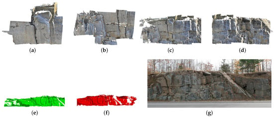
Figure 6.
Four different rock mass point clouds: (a) Rock1; (b) Rock2; (c,d) two different data of Rock3; (e,f) two different data of Rock4; and (g) the corresponding image of Rock4.
To quantitatively evaluate the registration results, the Root Mean Square Error (RMSE) [15] was used as the evaluation metric. The RMSE represents the root mean square distance of the corresponding point pair after the registration of two point clouds, which is defined as follows:
where N represents the number of points in the overlapping part and and represent the corresponding point pairs in the overlapping part.
4.3. Robustness Test
As some typical registration algorithms are very sensitive to the initial position of the point cloud, we chose Rock1 for experiments under different initial positions, in order to verify the robustness of the proposed method to the initial position.
Figure 7 shows the distribution of the distance between four different locations in the source point cloud and the target point cloud. Figure 8a–d illustrates the Rock1 point cloud at different positions and angles. Figure 8e shows the final registration results of the proposed method. It can be seen that our method had strong robustness to the initial position and angle of the point cloud. This was because the proposed method is based on the use of “candidate corner points” to complete the registration. The relative position of the feature point within the point cloud did not change with the change of the point cloud angle and position.
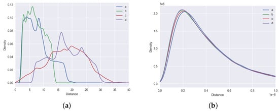
Figure 7.
Distribution of the distance between four different locations in the source point cloud and the target point cloud: (a,b) the distance distributions before and after registration, respectively. The letters a–d in the figure correspond to Figure 8a–d, respectively.

Figure 8.
The results of registration for Rock1 with different positions: (a–d) the four different positions of Rock1; and (e) the final results. The green color indicates the source point clouds with different positions. As the final results are almost identical, only one set of results is shown.
We also considered the robustness of the proposed method to point clouds with different overlap ratios and conducted an experimental verification. As shown in the first row of Figure 9, we took 20%, 25%, 50%, and 70% of the original Rock2 point cloud as the source point cloud. The location of the target point cloud was random, and the final registration results are displayed in the second row. It can be seen that the proposed method was robust to both different overlap rates and initial positions.
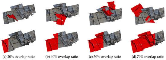
Figure 9.
The results of registration for Rock2 with different overlap ratios: (a) Rock2 with 20% overlap ratio; (b) Rock2 with 40% overlap ratio; (c) Rock2 with 50% overlap ratio; and (d) Rock2 with 70% overlap ratio.
4.4. Analysis of Registration Results for Rock Mass
Figure 10 shows the registration results for three sets of point clouds by different methods. Figure 10a–c presents the registration results of Rock1, Rock2, and Rock3, respectively. The first row in this figure presents the original position of the three sets of point clouds, while the remaining rows present the registration results of each method.
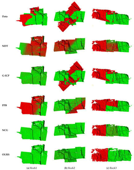
Figure 10.
Comparison of registration results by different methods for (a) Rock1, (b) Rock2, and (c) Rock3. The red color indicates the original point cloud, while green indicates the target point cloud.
As shown in Figure 10, the G-ICP method failed to register the Rock2 and Rock3 point clouds. This was because the G-ICP method is not robust to the initial position and angle of the point cloud. When the position or angle of the source point cloud and target point cloud significantly differed, the final registration result of G-ICP method was unsatisfactory, due to the local optima problem. The NDT method had a good registration effect on the Rock1 and Rock2 point clouds, which underwent rigid body transformations, but it was not ideal for the two Rock3 point clouds with overlapping parts. The plane characteristics of the overlapping part in Rock3 were weak, but the PPB method is based on plane extraction to find the corresponding relationship; thus, the PPB method failed to register the Rock3 point cloud. For the Rock2 and Rock3 point clouds, the NCG method obtained good results, but there was a slight dislocation in Rock1. The final registration results of the proposed method were all visually ideal.
Figure 11 illustrates the registration results for the Rock4 point cloud by the different methods. From a visual point of view, the registration of NDT and G-ICP for Rock4 failed, while the registration result of NCG was not ideal. There was a certain error in the overlap of the two point clouds, and they were not completely aligned. The PPB method had a slight dislocation. The final registration of the proposed method demonstrated that it can complete the registration work well.
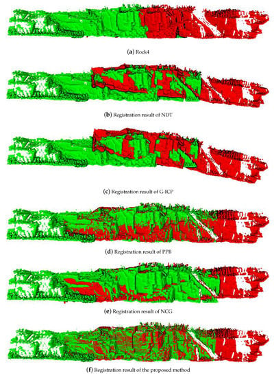
Figure 11.
The registration results of different methods for Rock4. (a) is the input point cloud, (b–f) are NDT, G-ICP, PPB, NCG and the proposed method registration results, respectively. The red and green colors represent the original point cloud and the target point cloud.
Observing the RMSE error in Table 3, we can see that the G-ICP method had a large RMSE error, due to multiple registration failures. The NDT method’s registration results for Rock1 and Rock2 were visually successful (see Figure 10), but its RMSE error was relatively large. This was because the NDT method is based on the use of statistical information to complete the initial registration, but no further ICP algorithm is used for optimization.

Table 3.
RMSEs(m) of the four compared methods for each point cloud.
Table 3 shows that PPB method had higher errors for Rock1, Rock2, and Rock4, and failed to register Rock3. This was because the PPB method uses the relationship between the areas of extracted planes to find the corresponding relationship during registration, and the results of plane extraction have a greater impact on registration. The registration error of the NCG method for the four point cloud sets was small. Table 3 and Table 4 fully show that the efficiency and accuracy of the proposed registration method are ideal.

Table 4.
Time consumption(s) of four methods for each point cloud.
4.5. Runtime Analysis
Table 4 shows the registration time of different methods for the four sets of point clouds. The table shows that the NDT and G-ICP methods were inefficient. When the number of points reached millions (Rock3 and Rock4), these two methods were less practical, due to their lower efficiency. The efficiency of the NCG method was lower than that of PPB and our method. In Rock3 and Rock4, our method had lower time complexity than the other methods. This was because the PPB method needs to compare the corresponding relationship of each plane, and there were more planes in Rock3 and Rock4. The difference was that our method only focuses on cluster sets, where the matching of such cluster sets is efficient.
5. Discussion
3D point cloud registration has become one of the key research hotspots in the field of remote sensing in recent years. Our research was carried out using the public dataset Rockbench [41]. From feature point extraction to the final registration process, a series of new ideas was implemented.
The comprehensive display of the experimental results demonstrates that the proposed method has high accuracy and efficiency in the registration of rock mass point clouds, mainly due to the following factors:
- (1)
- Efficient and accurate selection of points of interest. Starting from the prior knowledge that feature points are usually located in regions with drastic changes (e.g., the four types of feature regions introduced in Section 3.1), by using the relationship between the center point and the neighboring points to form a vector, the points in the feature region are effectively selected out. After this process, only a small number of points of interest is retained, which greatly reduces the amount of further calculations.
- (2)
- Efficient matching method. Point of interest matching is essential for finding the similarity between points of interest. We found that the geometry formed by the point and its neighbors after rotation has an invariant quantity, which allows a local point set to be considered as a whole, rather than just considering the individual point. In addition, the comparison of invariants on multiple scales improves the robustness of the method.
- (3)
- Fine adjustment of point position. After finding the corresponding point, fine-tuning of the point can align the position of the feature point. This step further improves the accuracy of the proposed method.
From visual observation (Figure 10 and Figure 11), there was almost no ghosting (ghosting is the visual effect of two corresponding planes that do not completely overlap) in our method, but there were some ghosts in the sampling contrast method. In the quantitative analysis (Table 3), our method had an accuracy an order of magnitude higher than that of the compared methods, as well as having certain advantages in speed.
However, the method still has some areas that can be improved. There are multiple steps in the whole method, with several parameters involved in each stage. Adjusting these parameters is cumbersome and has an impact on the final result. Simplifying the steps and the setting of adaptive parameters may be an important research direction. The choice of a single invariant is not stable enough. Although the comparison at multiple scales increased the robustness, it still required many attempts in a more complex environment. Finding and synthesizing other invariants to form a joint feature vector may help to improve the robustness of the method.
6. Conclusions
In this paper, we introduce, in a step-by-step manner, a new and effective method for rock mass point cloud registration. First, we define four types of rock mass points as points of interest. Then, using the feature of positive correlation between the points of interest and the vector composed of their neighboring points, it is judged that the sum of these vectors will have a larger modulus, such that the points with a larger modulus of the sum vector are retained as interest points. The method avoids complex calculations, has high efficiency, and can effectively extract the four types of points of interest. Second, we prove that there are specific invariants between feature point sets that have corresponding relationships and use this fact to determine the correspondences between feature point sets. This method avoids constructing complex descriptors for each feature point and improves the efficiency of the algorithm. Finally, we judge the position relationship between the known feature points and the feature points to be corrected to determine the possible locations of the feature points to be corrected in the data, as a set of candidate locations. Then, the center of the point set closest to the point to be corrected is used as the corrected position of the point set. This method calibrates the position of the feature points and improves the accuracy of the algorithm. We analyze the experimental results qualitatively and quantitatively and summarize and explained the advantages of the proposed method. At the end, we discuss and point out some problems of the proposed method and briefly detail potential corresponding solutions.
The proposed method is based on the sharp features of the point cloud. Therefore, it is suitable for registration of point clouds with sharper features on the surface. For point clouds with few or no sharp features at all (e.g., if the overlapping part is a single plane), the proposed registration method is not applicable.
Author Contributions
All authors contributed extensively to the work presented in this paper. Y.W. (Yunbiao Wang) proposed the main method and implemented all the algorithms presented in this manuscript and wrote the paper. L.L. put forward important opinions on the selection of some algorithms and implemented the related algorithms for comparison. J.X. discussed the structure of the manuscript, revised the manuscript, named the method, supported this research, and supplied computers for experiments. Y.W. (Ying Wang) improved the manuscript, supported this research, and protected the research process. All authors have read and agreed to the published version of the manuscript.
Funding
This work was supported by the National Natural Science Foundation of China (U2003109), the Strategic Priority Research Program of the Chinese Academy of Sciences (No. XDA23090304), the Youth Innovation Promotion Association of the Chinese Academy of Sciences (Y201935), and the Fundamental Research Funds for the Central Universities.
Institutional Review Board Statement
Not applicable.
Informed Consent Statement
Not applicable.
Data Availability Statement
Data available in publicly accessible repository that does not issue DOIs. Publicly available datasets were analyzed in this study.
Acknowledgments
The authors thank the reviewers for their valuable comments and suggestions.
Conflicts of Interest
The authors declare no conflict of interest.
References
- Sturzenegger, M.; Stead, D. Close-range terrestrial digital photogrammetry and terrestrial laser scanning for discontinuity characterization on rock cuts. Eng. Geol. 2009, 106, 163–182. [Google Scholar] [CrossRef]
- Hu, L.; Xiao, J.; Wang, Y. An automatic 3D Registration method for rock mass point clouds based on plane detection and polygon matching. Vis. Comput. 2019, 36, 669–681. [Google Scholar] [CrossRef]
- Besl, P.J.; McKay, N.D. Method for Registration of 3-D Shapes. In Sensor Fusion IV: Control Paradigms and Data Structures; Schenker, P.S., Ed.; SPIE: Bellingham, WA, USA, 1992; Volume 1611, pp. 586–606. [Google Scholar] [CrossRef]
- Granger, S.; Pennec, X. Multi-scale EM-ICP: A fast and robust approach for surface registration. In Proceedings of the European Conference on Computer Vision, Copenhagen, Denmark, 28–31 May 2002; pp. 418–432. [Google Scholar]
- Pulli, K. Multiview registration for large data sets. In Proceedings of the Second International Conference on 3-D Digital Imaging and Modeling (Cat. No.PR00062), Ottawa, ON, Canada, 8 October 1999. [Google Scholar] [CrossRef]
- Bouaziz, S.; Tagliasacchi, A.; Pauly, M. Sparse Iterative Closest Point. In Proceedings of the Eleventh Eurographics/ACMSIGGRAPH Symposium on Geometry Processing, Genova, Italy, 3–5 July 2013; pp. 113–123. [Google Scholar]
- Mohammadzade, H.; Hatzinakos, D. Iterative closest normal point for 3D face recognition. IEEE Trans. Pattern Anal. Mach. Intell. 2013, 35, 381–397. [Google Scholar] [CrossRef] [PubMed]
- Segal, A.; Hähnel, D.; Thrun, S. Generalized-ICP. In Proceedings of the Robotics: Science and Systems V, Seattle, WA, USA, 28 June 28–1 July 2009; The MIT Press: Cambridge, MA, USA, 2009. [Google Scholar] [CrossRef]
- Chen, C.S.; Yi-Ping, H.; Cheng, J.B. A fast automatic method for registration of partially-overlapping range images. In Proceedings of the Sixth International Conference on Computer Vision (IEEE Cat. No.98CH36271), Bombay, India, 7 January 1998; pp. 242–248. [Google Scholar]
- Aiger, D.; Mitra, N.J.; Cohen-Or, D. 4-Points congruent sets for robust pairwise surface registration. ACM Trans. Graph. 2008, 27. [Google Scholar] [CrossRef]
- Mellado, N.; Aiger, D.; Mitra, N.J. Super 4PCS Fast Global Pointcloud Registration via Smart Indexing. Comput. Graph. Forum 2014, 33, 205–215. [Google Scholar] [CrossRef]
- Theiler, P.W.; Wegner, J.D.; Schindler, K. Keypoint-based 4-Points Congruent Sets–Automated marker-less registration of laser scans. ISPRS J. Photogramm. Remote Sens. 2014, 96, 149–163. [Google Scholar] [CrossRef]
- Mohamad, M.; Rappaport, D.; Greenspan, M. Generalized 4-Points Congruent Sets for 3D Registration. In Proceedings of the 2nd International Conference on 3D Vision, Tokyo, Japan, 8–11 December 2014; Volume 1, pp. 83–90. [Google Scholar] [CrossRef]
- Mohamad, M.; Ahmed, M.T.; Rappaport, D.; Greenspan, M. Super Generalized 4PCS for 3D Registration. In Proceedings of the 2015 International Conference on 3D Vision, Lyon, France, 19–22 October 2015; pp. 598–606. [Google Scholar] [CrossRef]
- Wang, F.; Xiao, J.; Wang, Y. Efficient Rock-mass Point Cloud Registration Using N-point Complete Graphs. IEEE Trans. Geosci. Remote Sens. 2019, 57, 9332–9343. [Google Scholar] [CrossRef]
- Rusu, R.B.; Marton, Z.C.; Blodow, N.; Beetz, M. Persistent point feature histograms for 3D point clouds. In Proceedings of the 10th International Conference on Intelligent Autonomous Syst (IAS-10), Baden-Baden, Germany, January 2008; pp. 119–128. [Google Scholar]
- Rusu, R.B.; Blodow, N.; Beetz, M. Fast Point Feature Histograms (FPFH) for 3D registration. In Proceedings of the 2009 IEEE International Conference on Robotics and Automation, Kobe, Japan, 12–17 May 2009; pp. 3212–3217. [Google Scholar] [CrossRef]
- Tombari, F.; Salti, S.; Di Stefano, L. Unique signatures of histograms for local surface description. In Proceedings of the European Conference on Computer Vision, Crete, Greece, 5–11 September 2010; pp. 356–369. [Google Scholar]
- Habib, A.; Ghanma, M.; Morgan, M.; Al-Ruzouq, R. Photogrammetric and LiDAR data registration using linear features. Photogramm. Eng. Remote Sens. 2005, 71, 699–707. [Google Scholar] [CrossRef]
- Al-Durgham, M.; Habib, A. A framework for the registration and segmentation of heterogeneous LiDAR data. Photogramm. Eng. Remote Sens. 2013, 79, 135–145. [Google Scholar] [CrossRef]
- Yang, B.; Zang, Y. Automated registration of dense terrestrial laser-scanning point clouds using curves. ISPRS J. Photogramm. Remote Sens. 2014, 95, 109–121. [Google Scholar] [CrossRef]
- Dold, C.; Brenner, C. Registration of terrestrial laser scanning data using planar patches and image data. Int. Arch. Photogramm. Remote Sens. Spat. Inf. Sci. ISPRS Arch. 2006, 36, 78–83. [Google Scholar]
- Huang, J.; Kwok, T.H.; Zhou, C. V4PCS: Volumetric 4PCS algorithm for global registration. J. Mech. Des. 2017, 139. [Google Scholar] [CrossRef]
- Zeng, A.; Song, S.; Nießner, M.; Fisher, M.; Xiao, J.; Funkhouser, T. 3dmatch: Learning local geometric descriptors from rgb-d reconstructions. In Proceedings of the IEEE Conference on Computer Vision and Pattern Recognition, Honolulu, HI, USA, 21–26 July 2017; pp. 1802–1811. [Google Scholar]
- Gojcic, Z.; Zhou, C.; Wegner, J.D.; Wieser, A. The perfect match: 3d point cloud matching with smoothed densities. In Proceedings of the IEEE Conference on Computer Vision and Pattern Recognition, Long Beach, CA, USA, 16–20 June 2019; pp. 5545–5554. [Google Scholar]
- Wang, Y.; Solomon, J.M. Deep closest point: Learning representations for point cloud registration. In Proceedings of the IEEE International Conference on Computer Vision, Seoul, Korea, 27 October–2 November 2019; pp. 3523–3532. [Google Scholar]
- Aoki, Y.; Goforth, H.; Srivatsan, R.A.; Lucey, S. Pointnetlk: Robust & efficient point cloud registration using pointnet. In Proceedings of the IEEE Conference on Computer Vision and Pattern Recognition, Long Beach, CA, USA, 16–20 June 2019; pp. 7163–7172. [Google Scholar]
- Qi, C.R.; Su, H.; Mo, K.; Guibas, L.J. Pointnet: Deep learning on point sets for 3d classification and segmentation. In Proceedings of the IEEE Conference on Computer Vision and Pattern Recognition, Honolulu, HI, USA, 21–26 July 2017; pp. 652–660. [Google Scholar]
- Lucas, B.D.; Kanade, T. An Iterative Image Registration Technique with an Application to Stereo Vision. In Proceedings of the 7th International Joint Conference on Artificial Intelligence, Vancouver, BC, Canada, 24–28 August 1981; pp. 674–679. [Google Scholar]
- Fitzgibbon, A.W. Robust registration of 2D and 3D point sets. Image Vis. Comput. 2003, 21, 1145–1153. [Google Scholar] [CrossRef]
- Chetverikov, D.; Svirko, D.; Stepanov, D.; Krsek, P. The trimmed iterative closest point algorithm. In Proceedings of the Object Recognition Supported by User Interaction for Service Robots, Quebec City, QC, Canada, 11–15 August 2002; Volume 3, pp. 545–548. [Google Scholar]
- Mavridis, P.; Andreadis, A.; Papaioannou, G. Efficient sparse icp. Comput. Aided Geom. Des. 2015, 35, 16–26. [Google Scholar] [CrossRef]
- Grant, D.; Bethel, J.; Crawford, M. Point-to-plane registration of terrestrial laser scans. ISPRS J. Photogramm. Remote Sens. 2012, 72, 16–26. [Google Scholar] [CrossRef]
- Censi, A. An ICP variant using a point-to-line metric. In Proceedings of the 2008 IEEE International Conference on Robotics and Automation, Pasadena, CA, USA, 19–23 May 2008; pp. 19–25. [Google Scholar]
- Rusinkiewicz, S. A symmetric objective function for ICP. ACM Trans. Graph. (TOG) 2019, 38, 1–7. [Google Scholar] [CrossRef]
- Magnusson, M.; Lilienthal, A.; Duckett, T. Scan registration for autonomous mining vehicles using 3D-NDT. J. Field Robot. 2007, 24, 803–827. [Google Scholar] [CrossRef]
- Gruen, A.; Akca, D. Least squares 3D surface and curve matching. ISPRS J. Photogramm. Remote Sens. 2005, 59, 151–174. [Google Scholar] [CrossRef]
- Jian, B.; Vemuri, B.C. A robust algorithm for point set registration using mixture of Gaussians. In Proceedings of the Tenth IEEE International Conference on Computer Vision (ICCV’05), Beijing, China, 17–21 October 2005; Volume 2, pp. 1246–1251. [Google Scholar]
- Pomerleau, F.; Colas, F.; Siegwart, R.; Magnenat, S. Comparing ICP variants on real-world data sets. Auton. Robot. 2013, 34, 133–148. [Google Scholar] [CrossRef]
- Ester, M.; Kriegel, H.; Sander, J.; Xu, X. A Density-Based Algorithm for Discovering Clusters in Large Spatial Databases with Noise. In Proceedings of the Second International Conference on Knowledge Discovery and Data Mining (KDD-96), Portland, OR, USA, 2–4 August 1996; pp. 226–231. [Google Scholar]
- Rusu, R.B.; Cousins, S. 3D is here: Point Cloud Library (PCL). In Proceedings of the 2011 IEEE International Conference on Robotics and Automation, Shanghai, China, 9–13 May 2011; pp. 1–4. [Google Scholar] [CrossRef]
- Lato, M.; Kemeny, J.; Harrap, R.; Bevan, G. Rock bench: Establishing a common repository and standards for assessing rockmass characteristics using LiDAR and photogrammetry. Comput. Geosci. 2013, 50, 106–114. [Google Scholar] [CrossRef]
Publisher’s Note: MDPI stays neutral with regard to jurisdictional claims in published maps and institutional affiliations. |
© 2021 by the authors. Licensee MDPI, Basel, Switzerland. This article is an open access article distributed under the terms and conditions of the Creative Commons Attribution (CC BY) license (https://creativecommons.org/licenses/by/4.0/).
