
Evolution of Brightness and Color of the Night Sky in Madrid

 , ,
, ,  , and
, and
Abstract
1. Introduction
2. Materials and Methods
2.1. Background
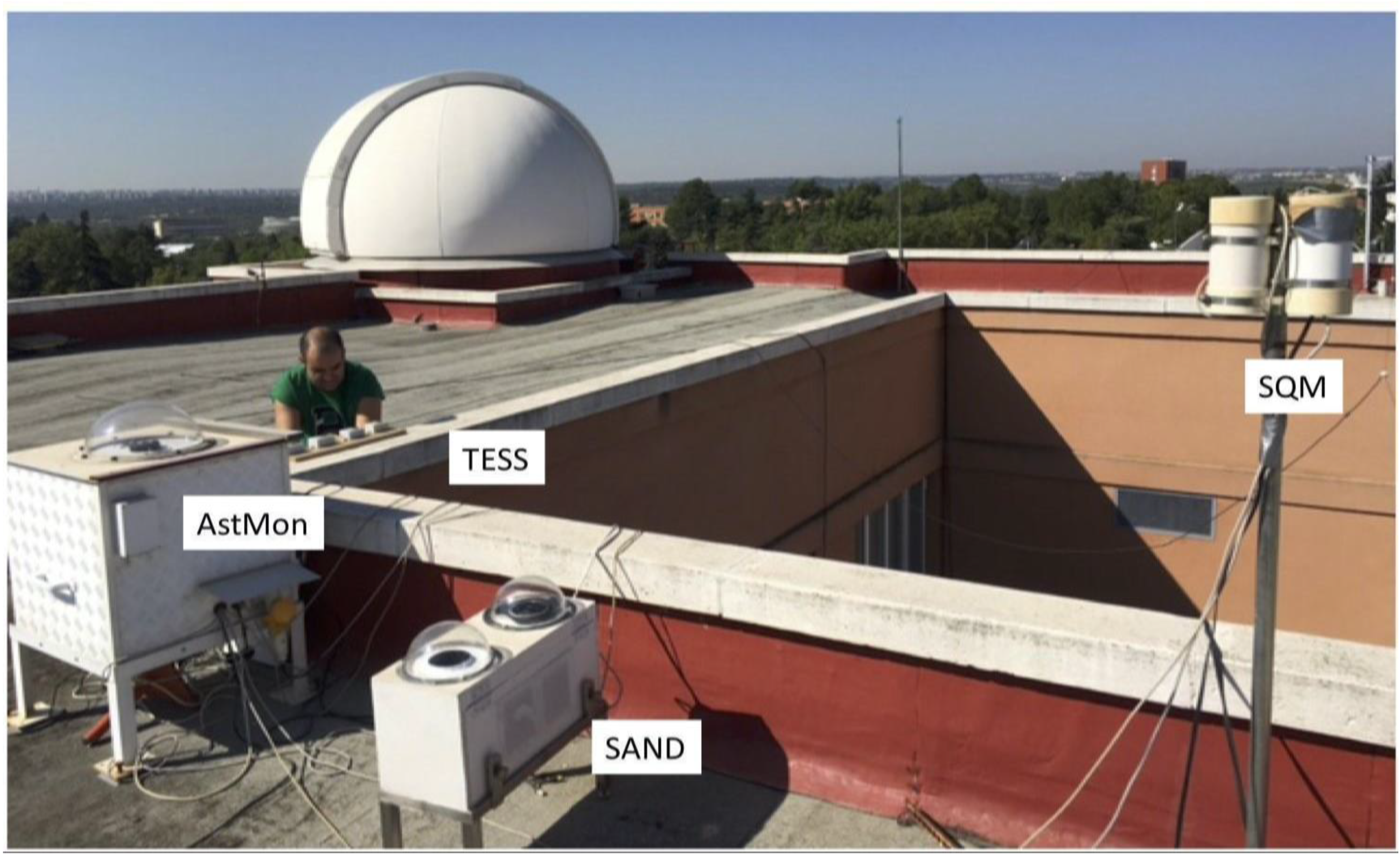
2.2. Available Data
2.3. Data Management and Pre-Processing
2.4. Filtering Process
3. Results
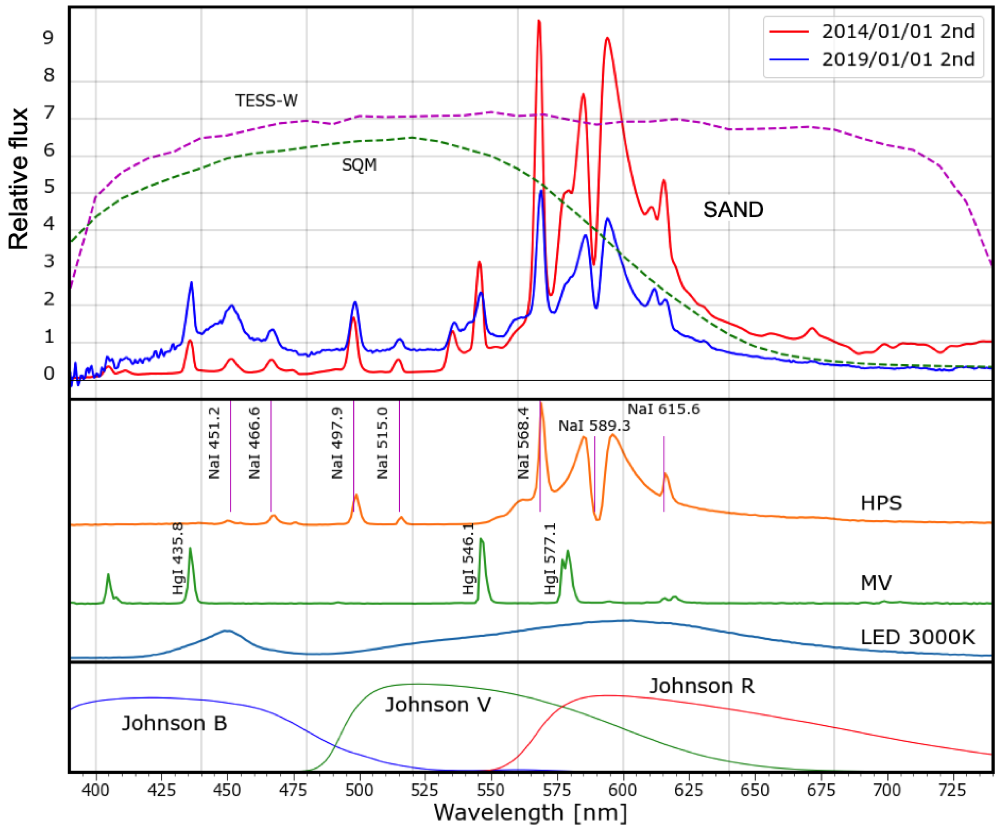
3.1. Madrid Night Sky Spectra
3.2. AstMon
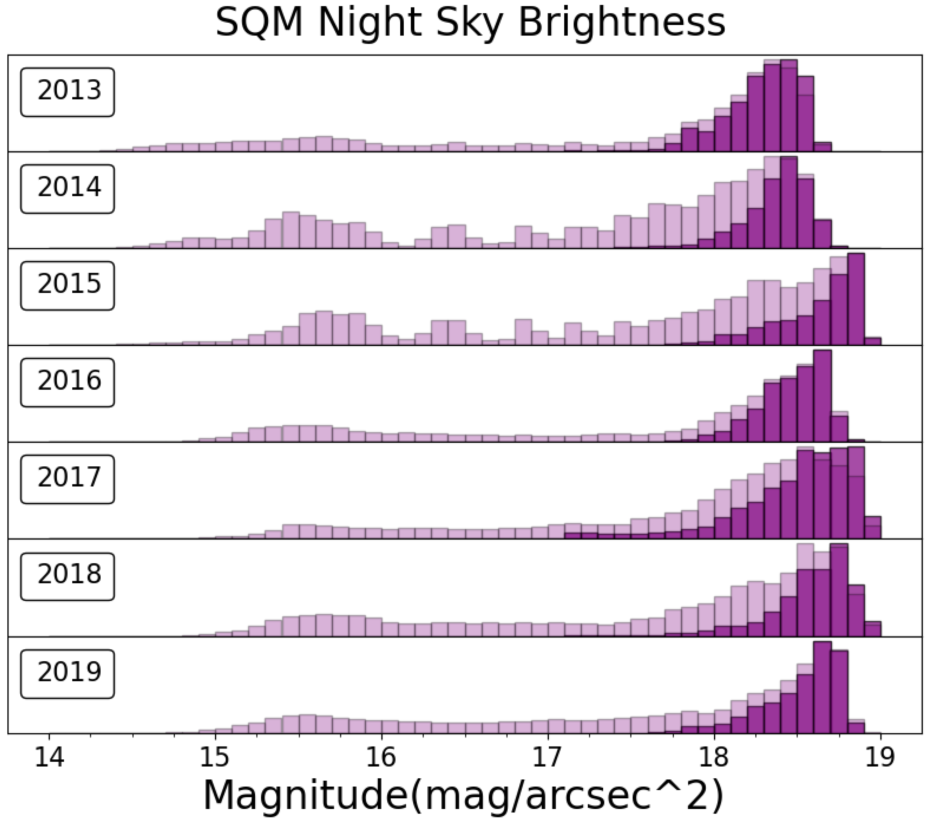
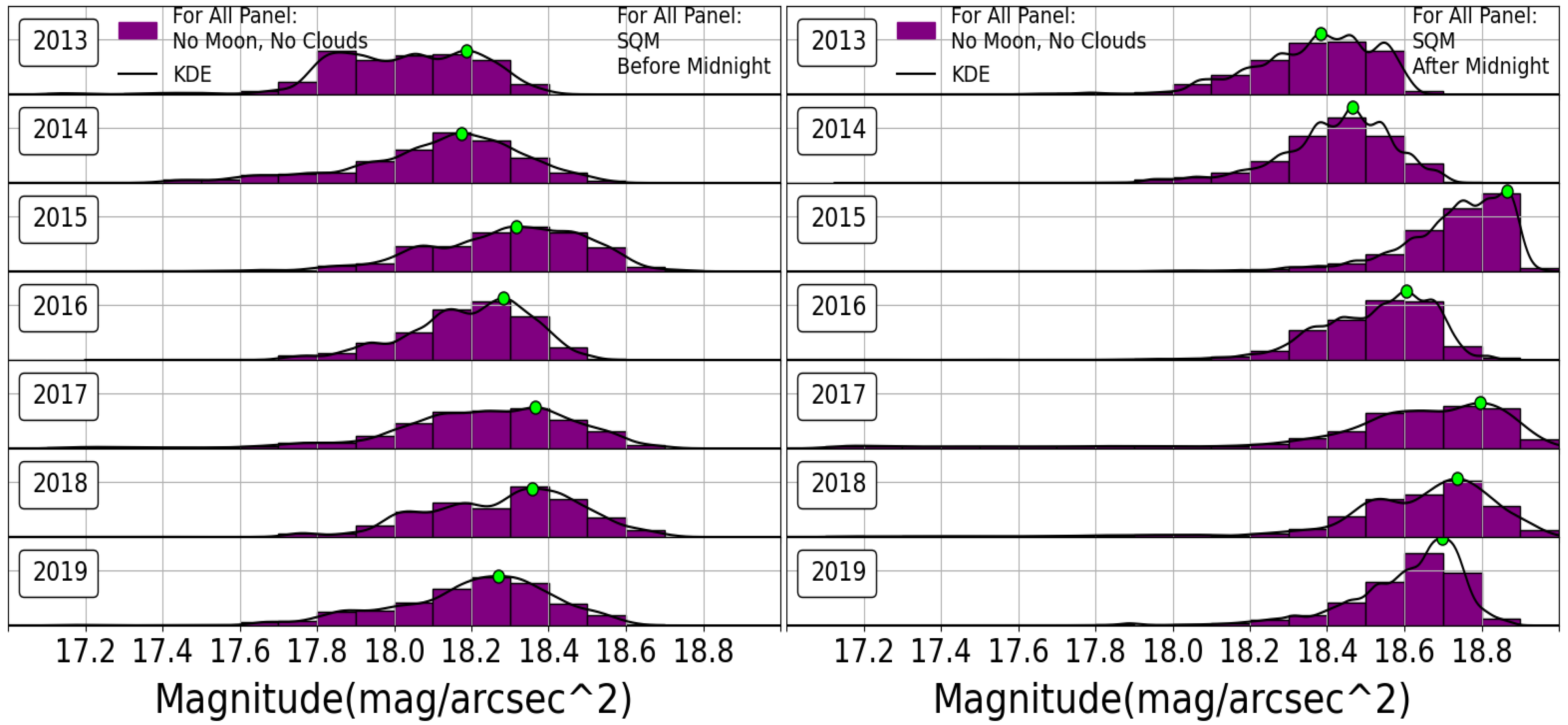
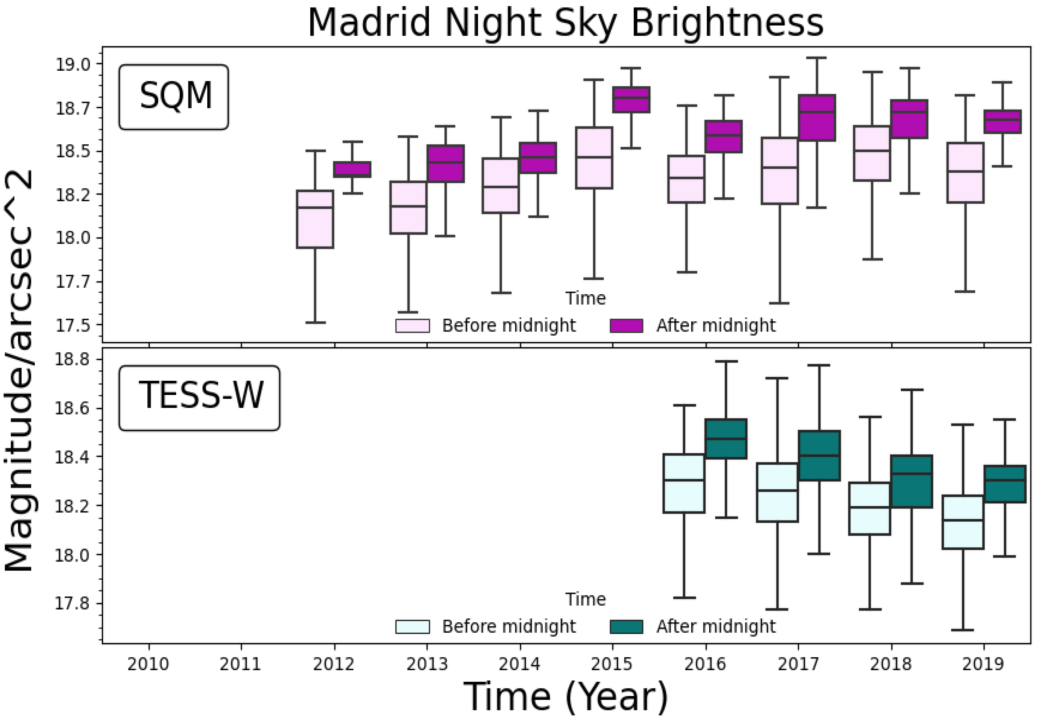
3.3. Sky Quality Meter SQM
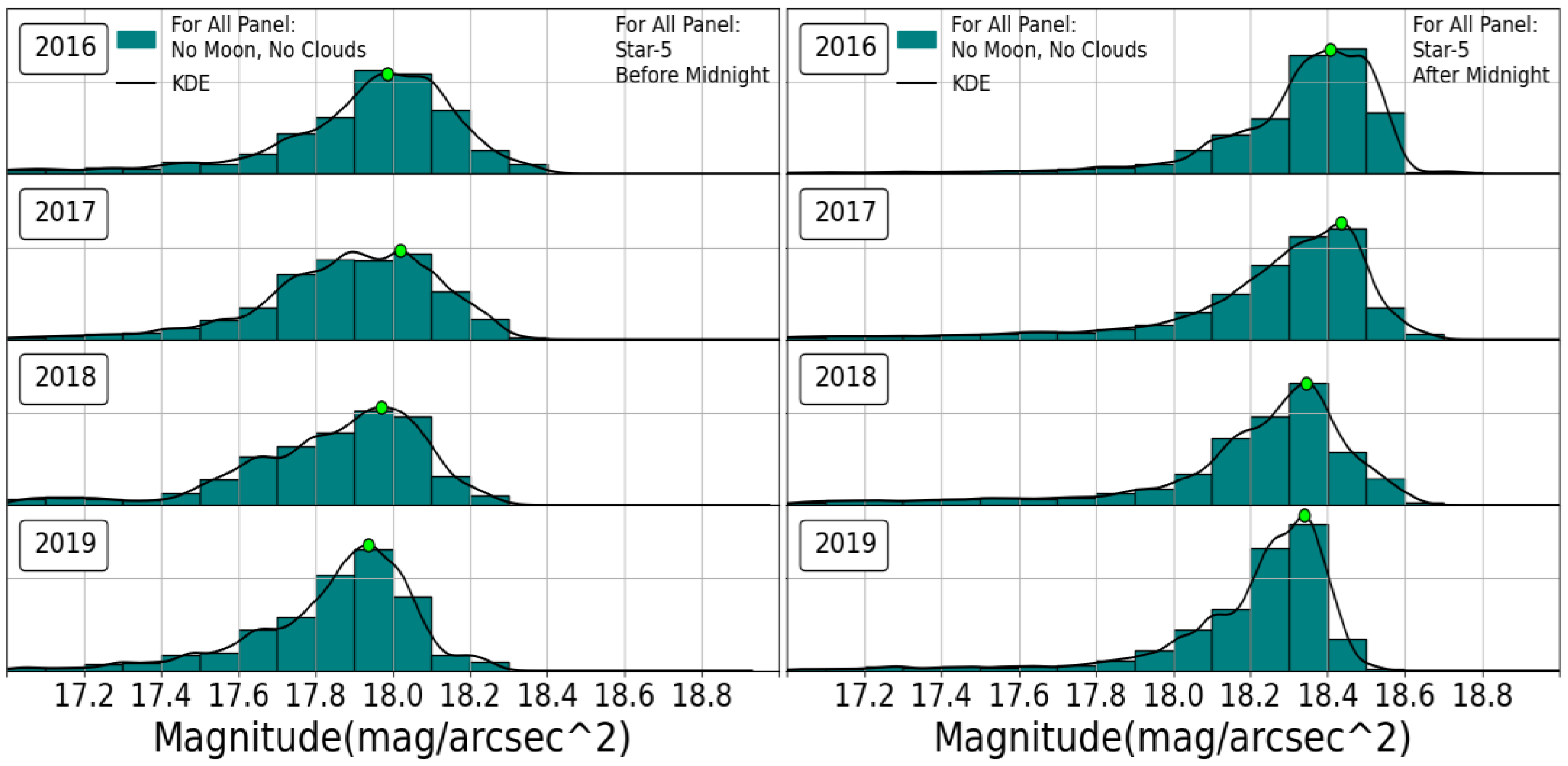
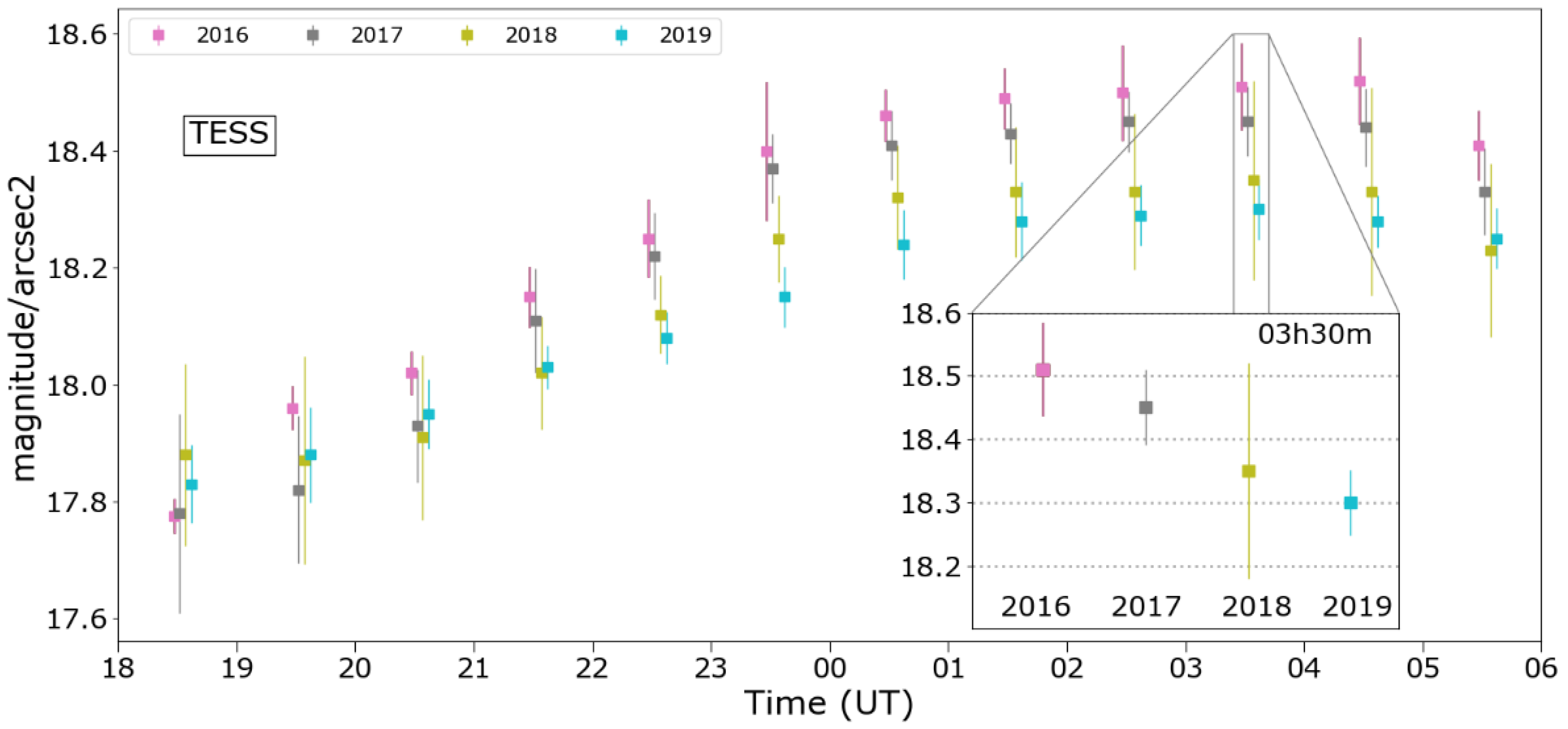
3.4. TESS-W
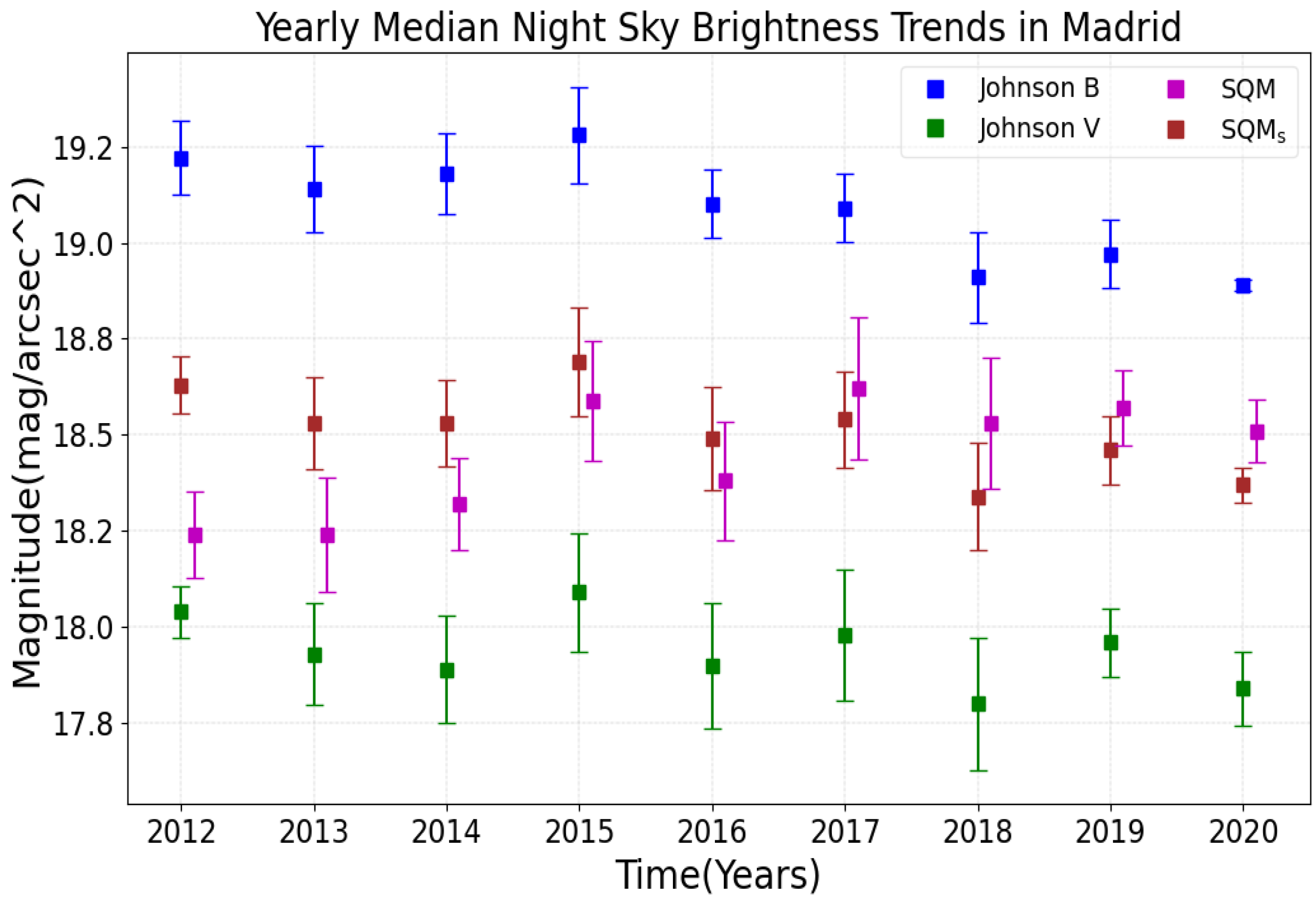
3.5. SQM and Johnson Photometry Comparison
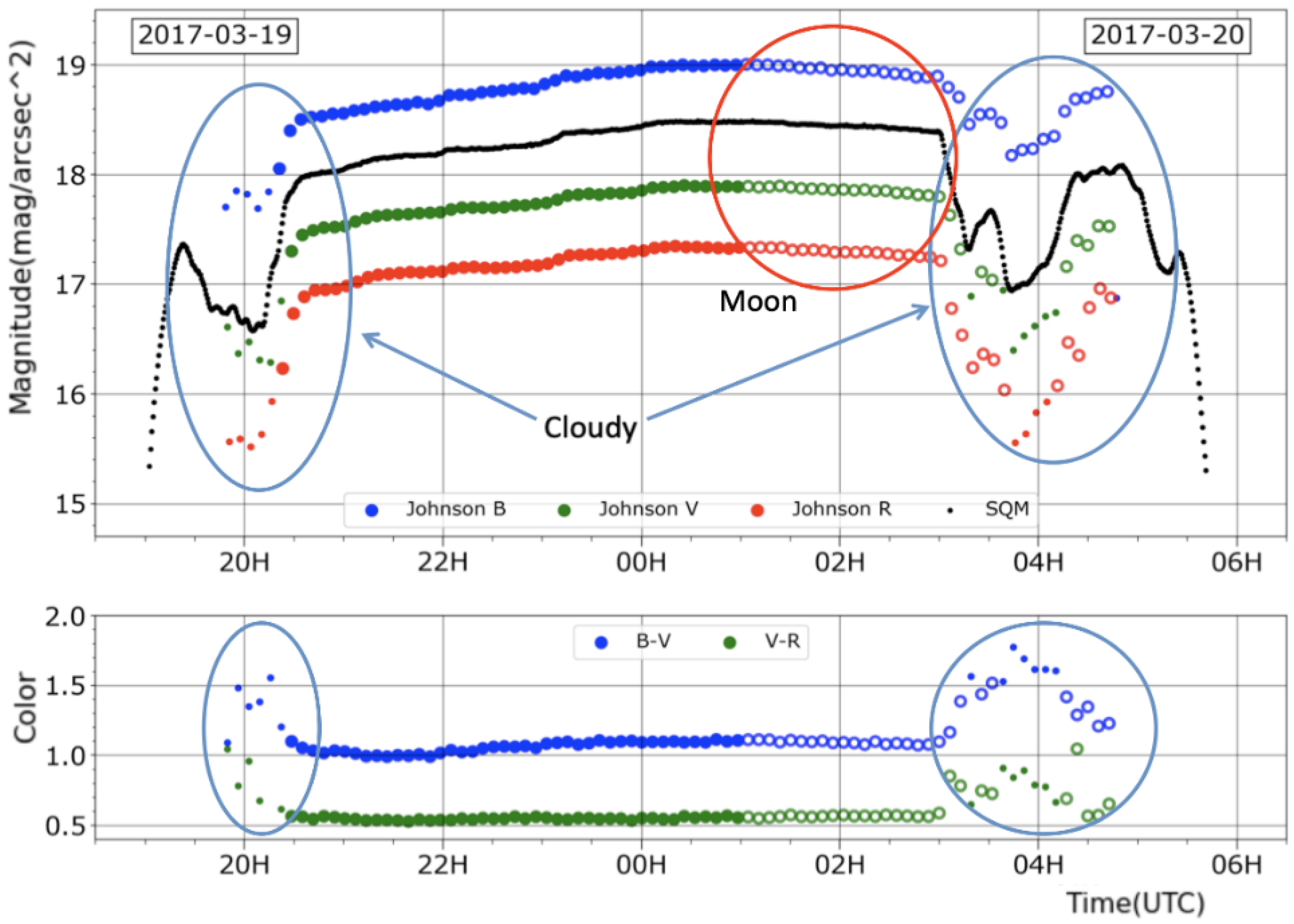
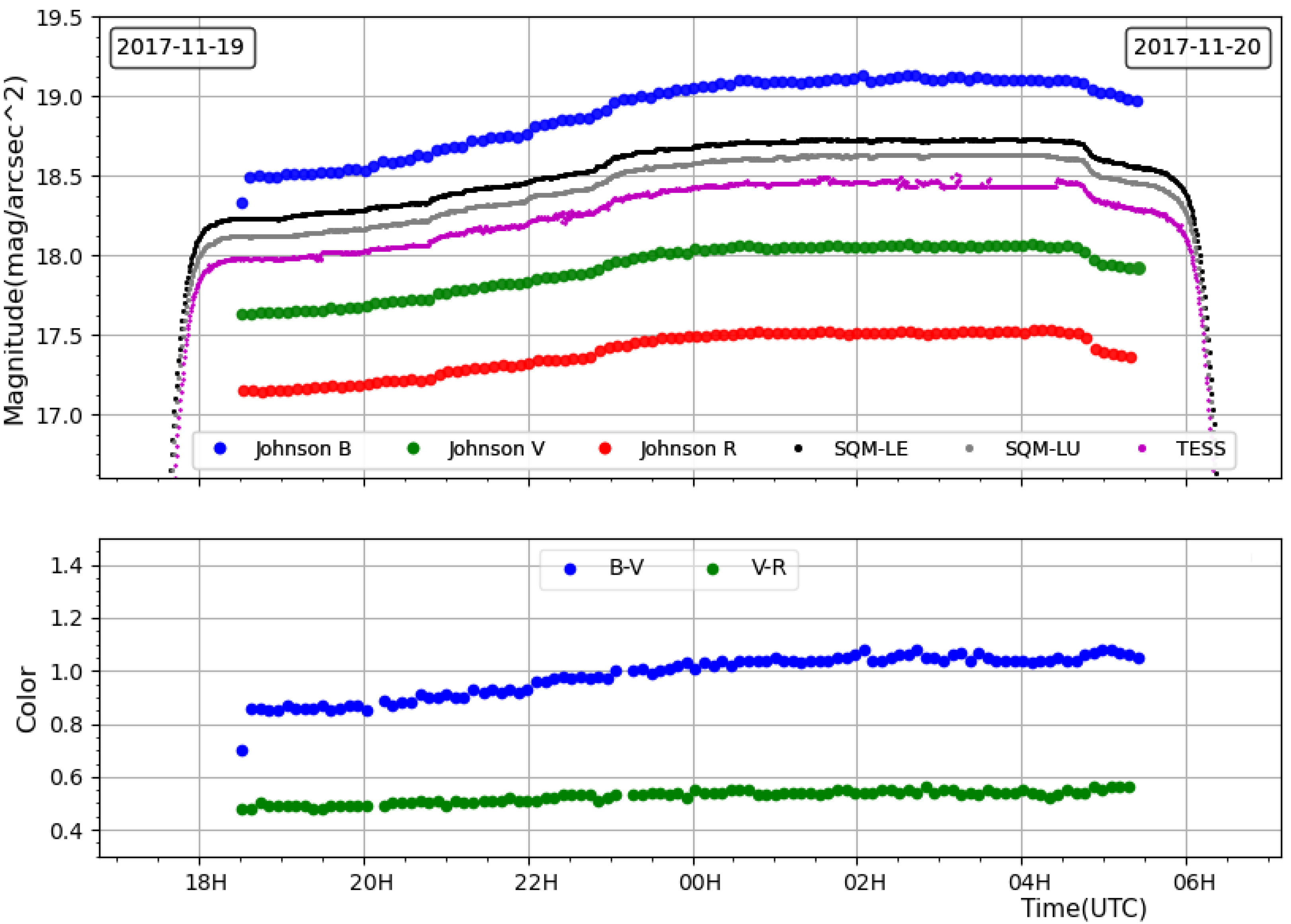
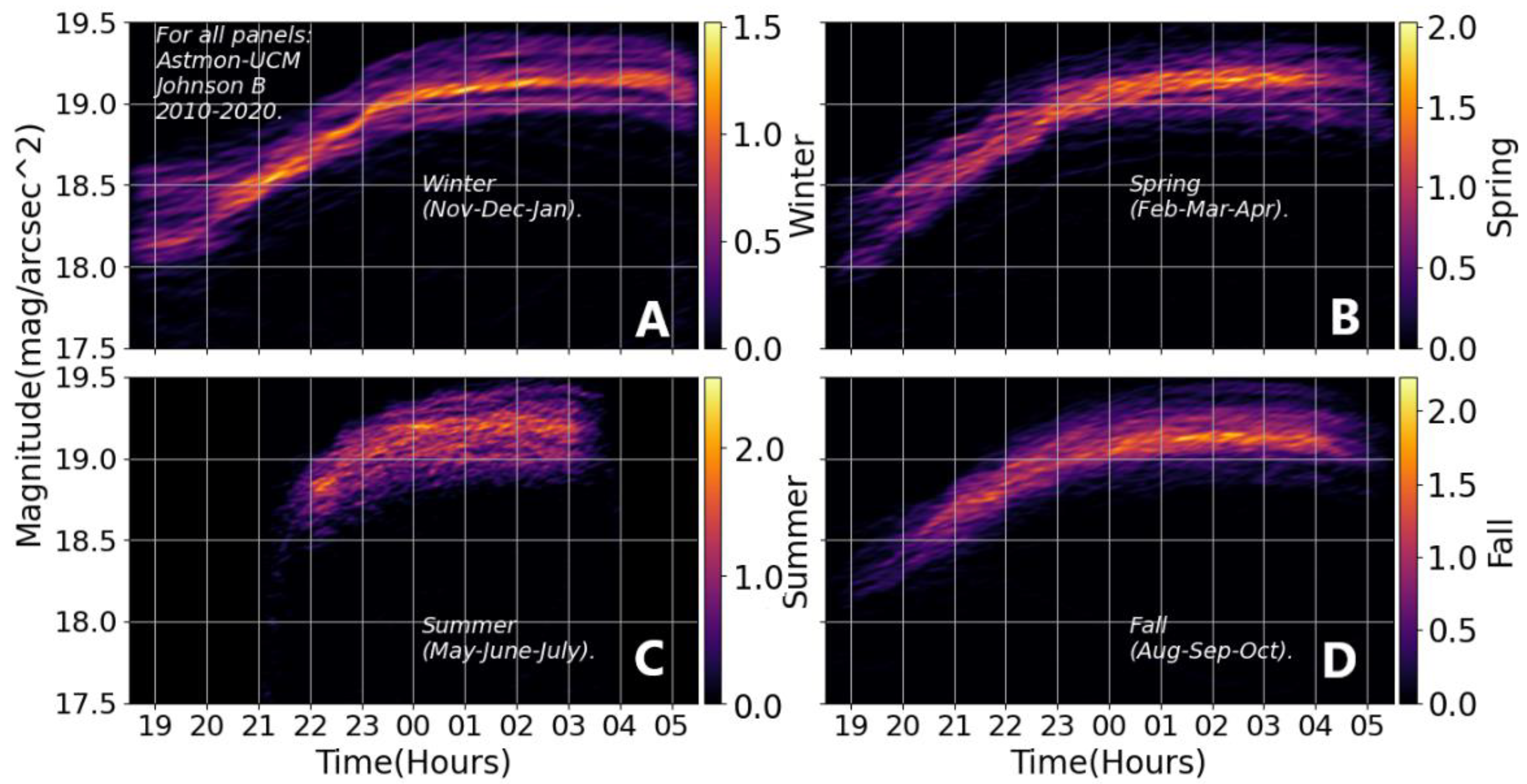
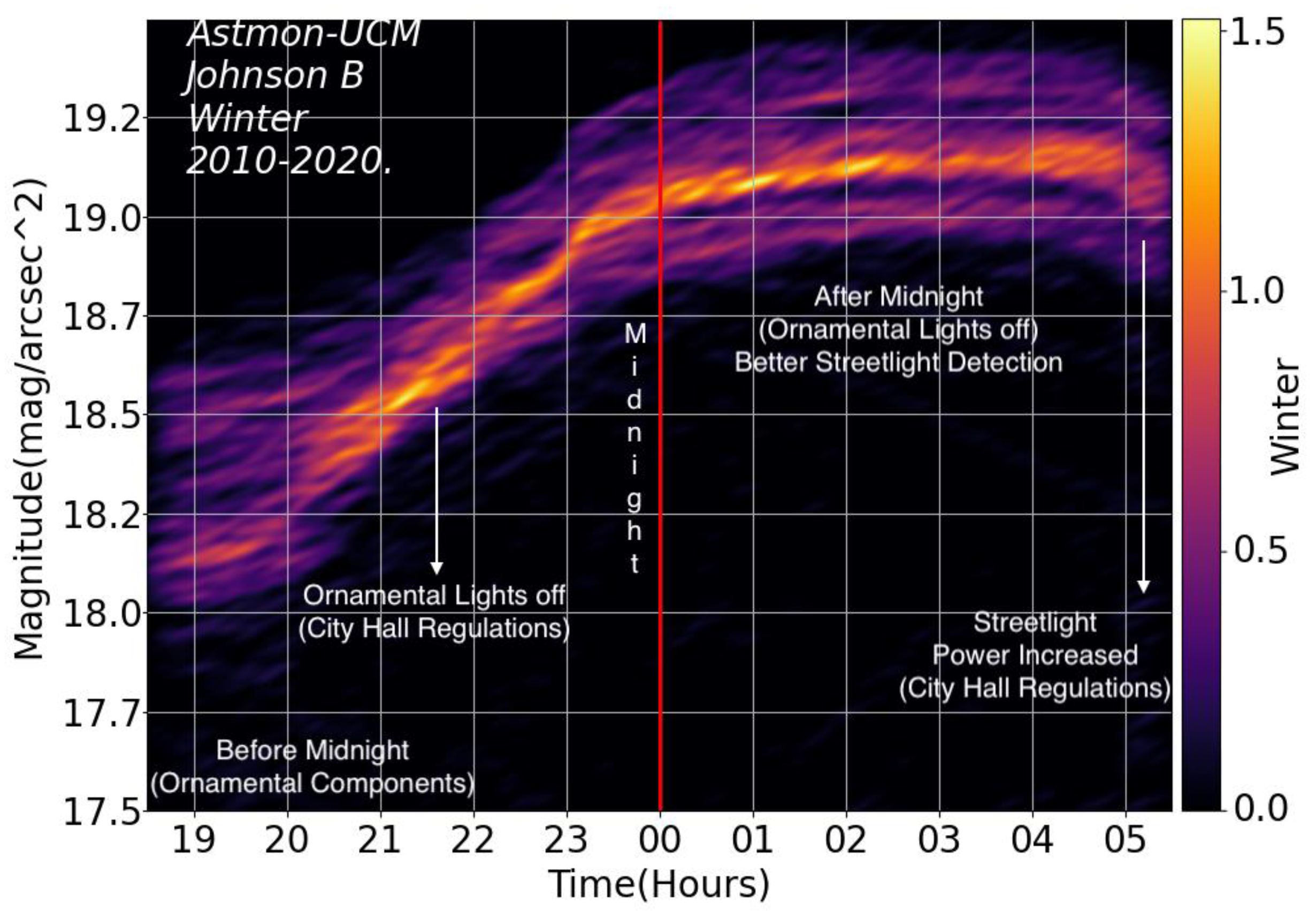
3.6. Variation throughout the Night
4. Discussion
4.1. Night Sky Brightness Changes over Time
4.1.1. SQM and TESS-W
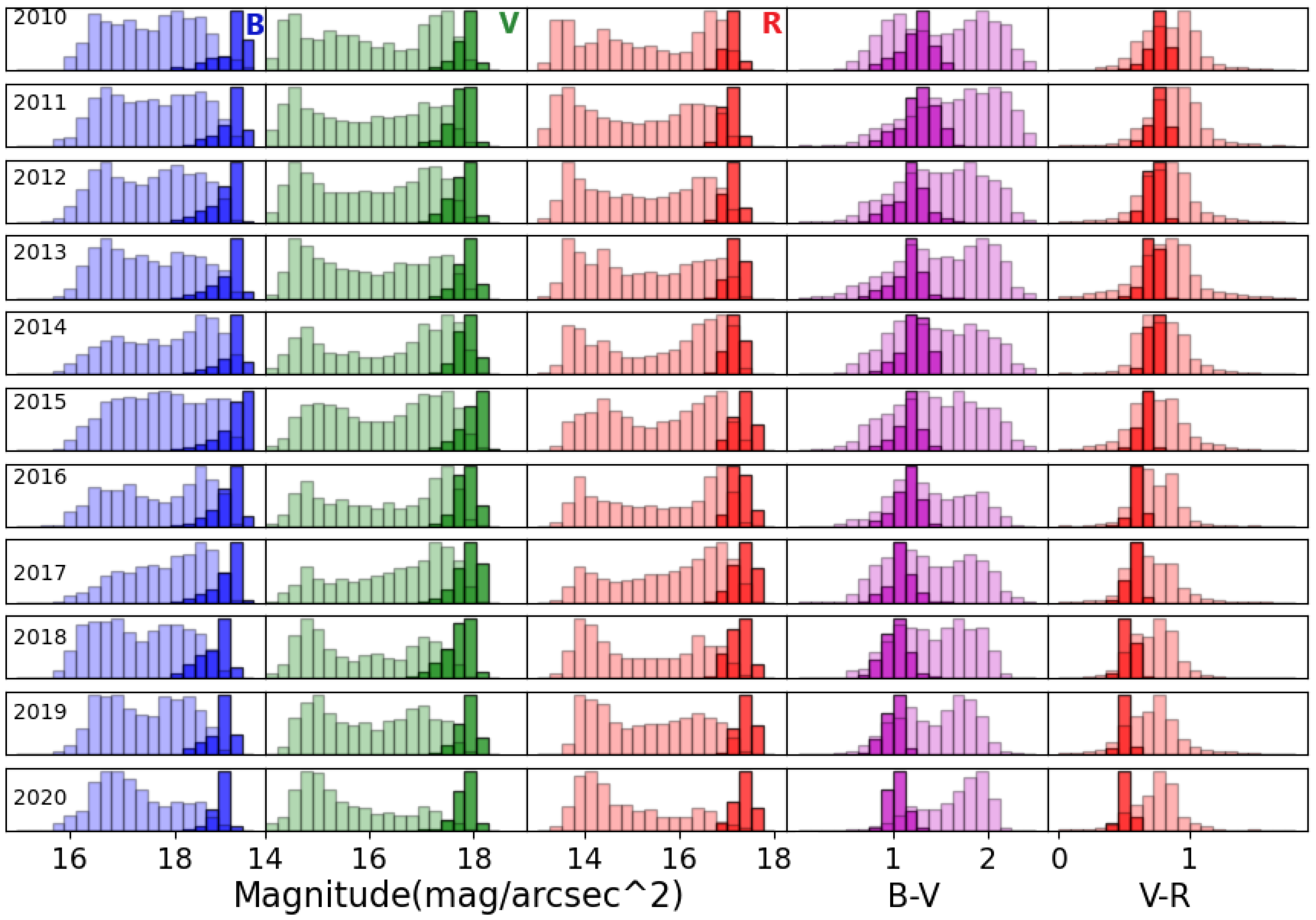
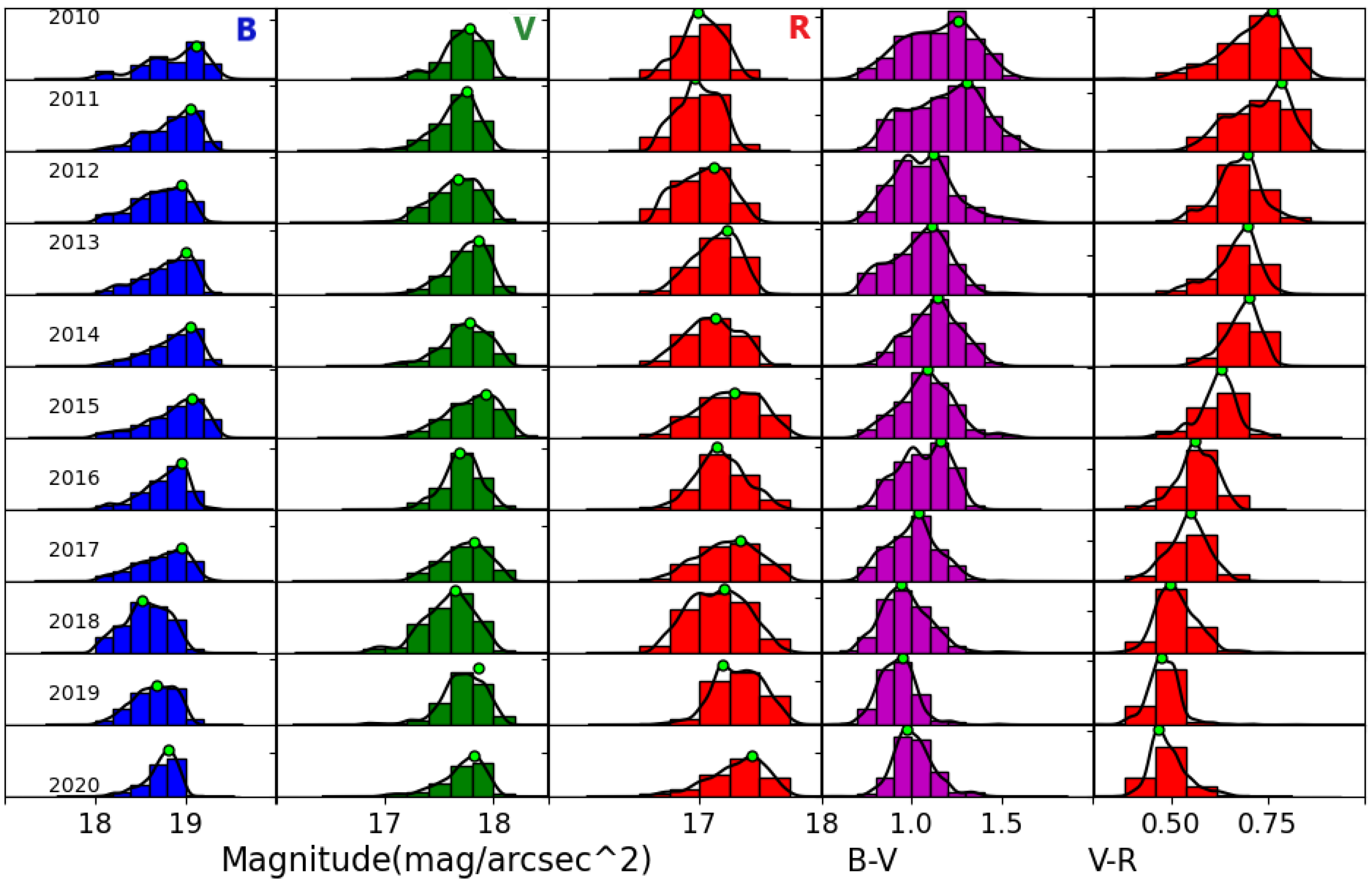
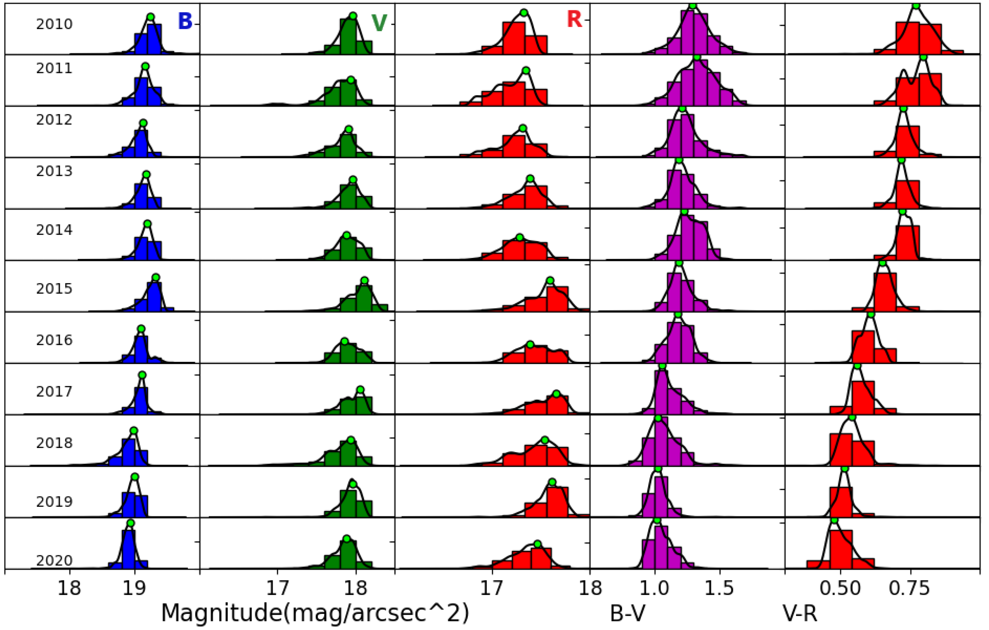
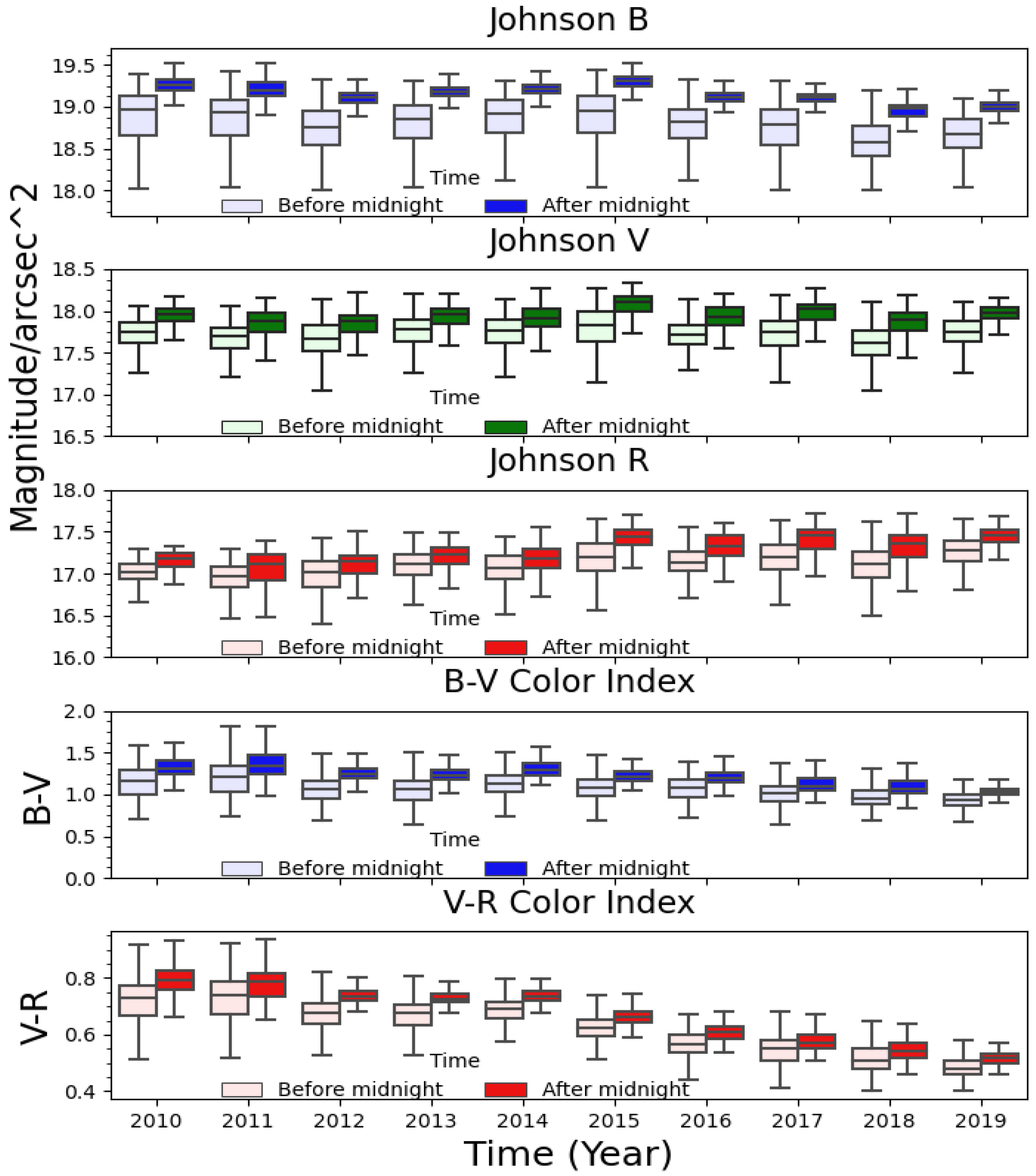
4.1.2. ASTMON Brightness and Color Evolution
4.1.3. Winter Curves
4.1.4. Comparison with Other Studies
5. Conclusions
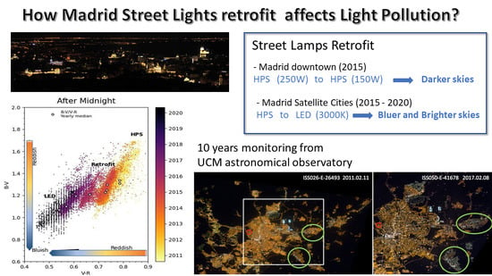
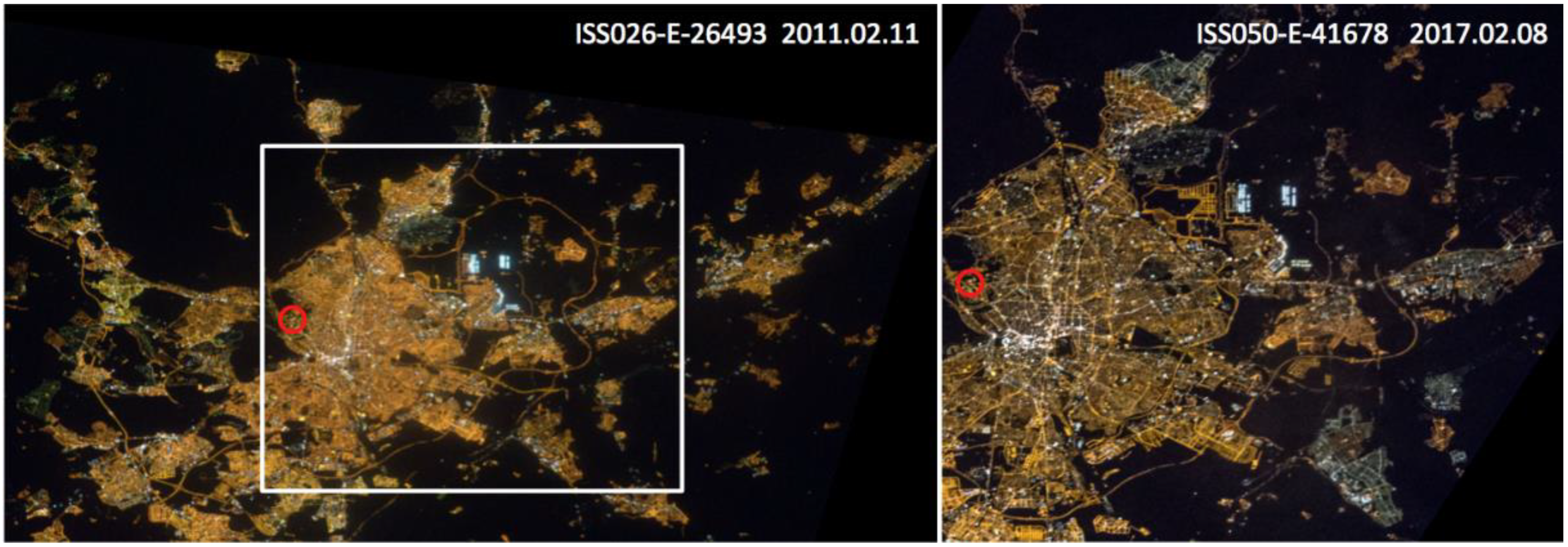
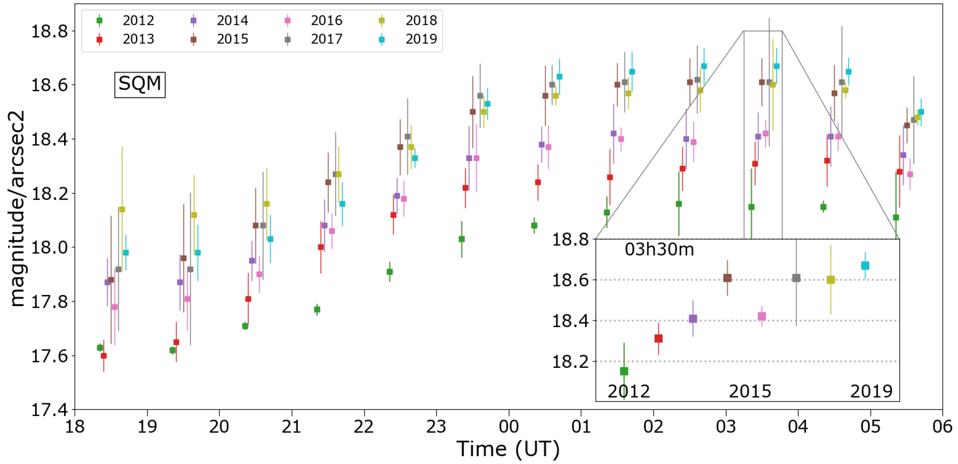
- A 38% darkening of the night sky from 2012 to 2019, as measured by SQM. After the streetlight retrofit in 2015, the SQM photometer did not follow the trends detected by AstMon in the Johnson V band and the broadband TESS-W photometer. Although the change in shifting lighting types could play a small role, the main effect is the loss of the SQM photometer sensitivity. This experimental outcome has far-reaching implications for long-term global monitoring of night sky brightness, if confirmed by similar studies.
- 2.
- A 10% brightening of the night sky from 2016 to 2019, as measured by TESS-W. This percentage value followed the trends of Johnson B and V photometric bands, as detected by AstMon.
- 3.
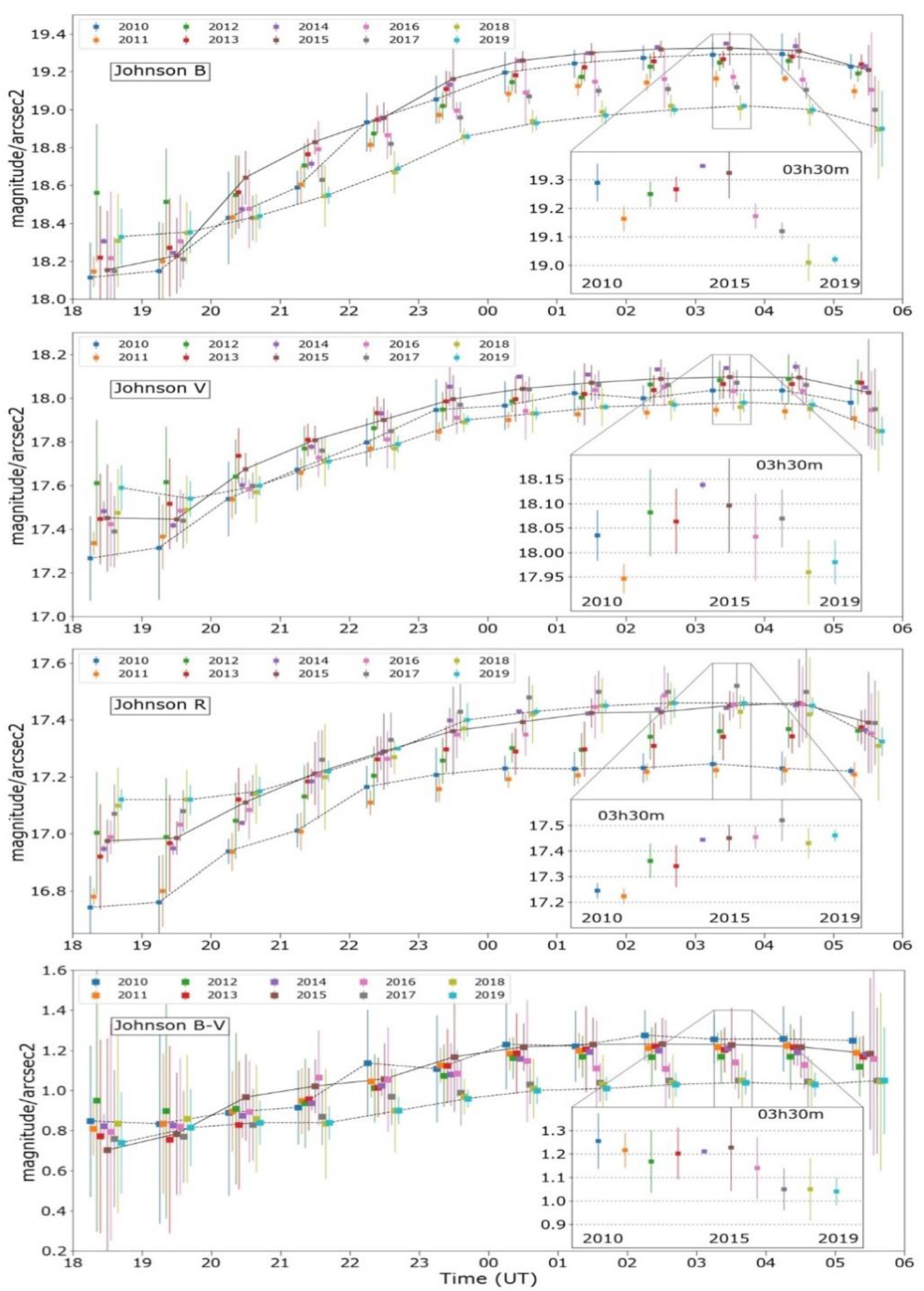
- We compared brightness trends in the Johnson photometric bands before and after the streetlight retrofit in 2015. The sky brightness detected in the Johnson B band darkened 14% from 2011 to 2015 and brightened by 32% from 2015 to 2019. The sky brightness detected in the Johnson V band darkened by 13% from 2011 to 2015 and brightened by 11% from 2015 to 2019. The sky brightness detected in the Johnson R band darkened by 19% from 2011 to 2015; it continued to darken from 2015 to 2019, darkening by 1% in this period. The Johnson B band reached its darkest values in 2015, while the Johnson V was darkest in 2014.
- 4.
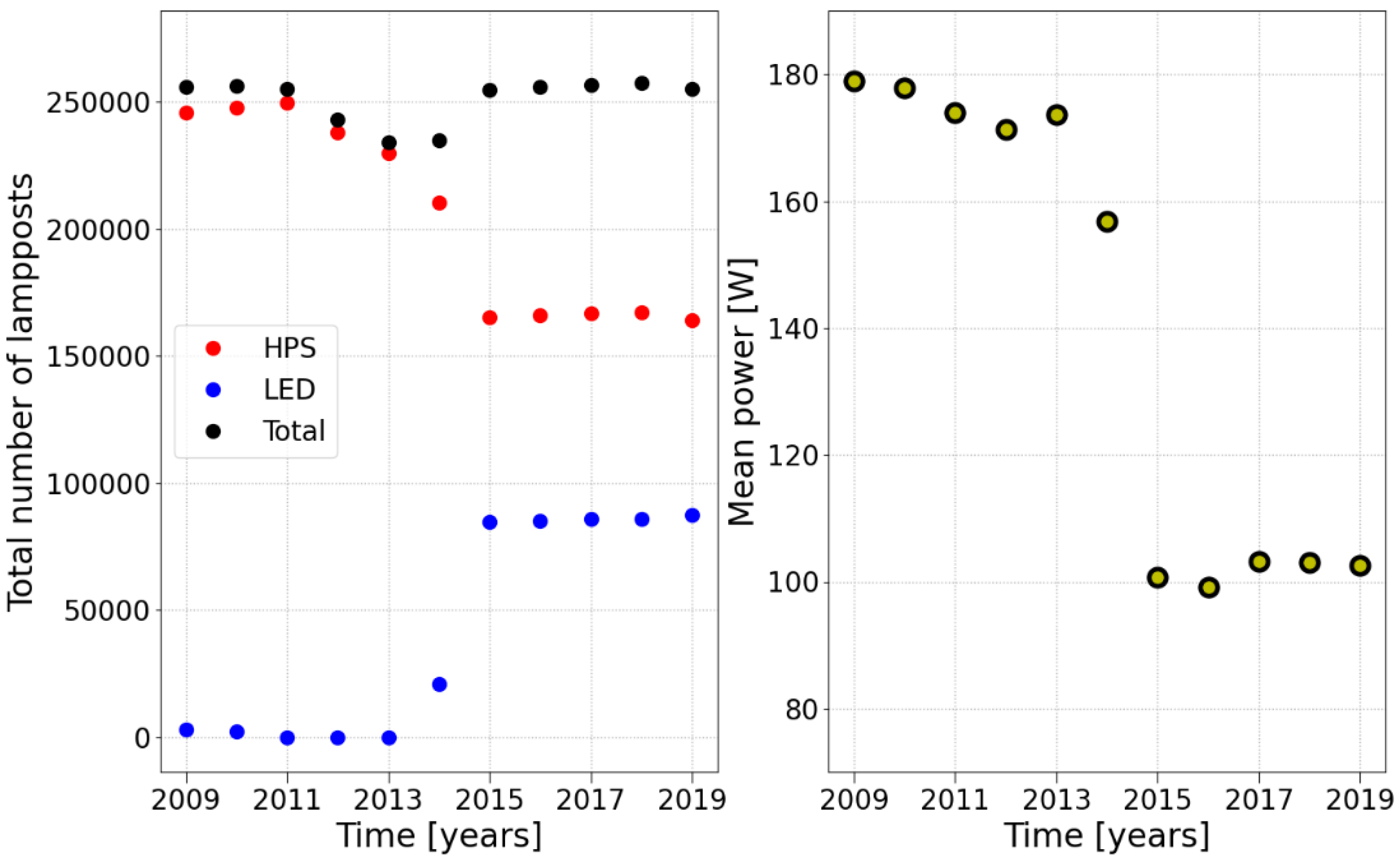
- Radiance in the Johnson R band decreased due to less abundant HPS technology, while radiance in the Johnson B band increased due to more abundant LED technology (at least until 2015).
- 5.
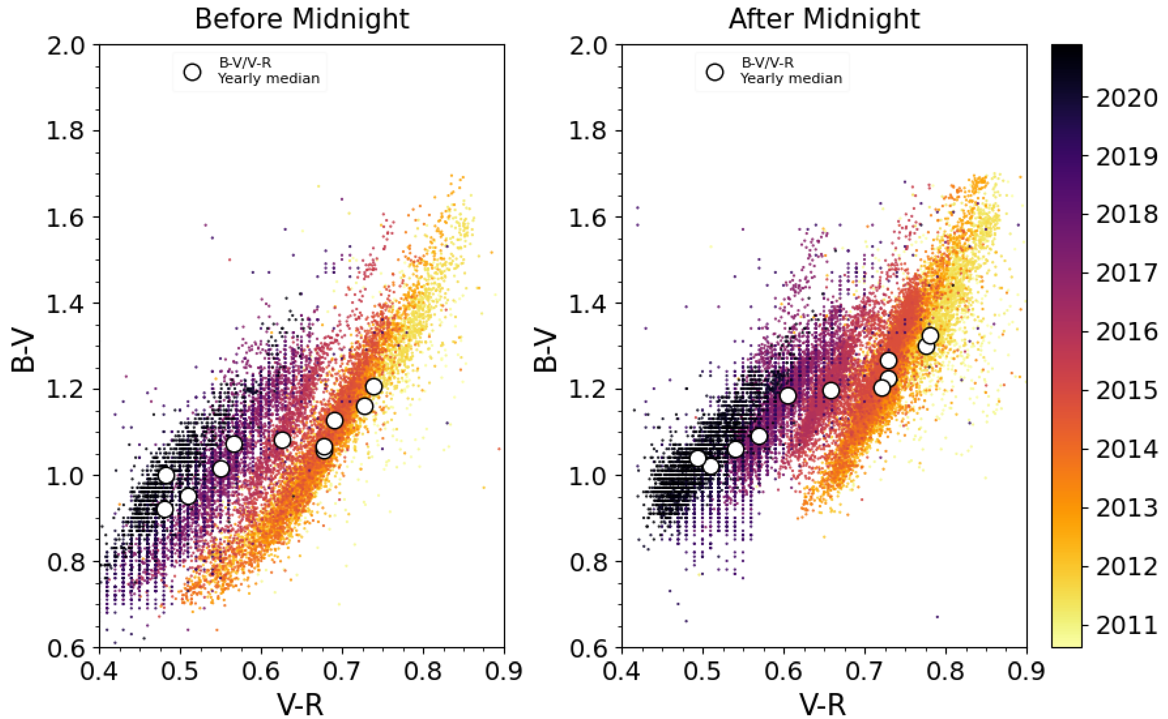
- Before midnight, we did not find a marked change in the winter color index. After midnight, following the streetlight retrofit in 2015, the color index shifted considerably toward bluer skies. Prior to the retrofit, there was a shift in the color of the Madrid night sky from bluish (B-V = 0.8) before midnight, to yellowish (B-V = 1.2) after midnight. After the retrofit, the difference in color before midnight (B-V = 0.8) and after midnight (B-V = 1.0) decreased.
- 6.
- The B-V and V-R yearly color indices showed a steady decrease in value from 2010 to 2019 (B-V = 1.24 ± 0.09 to 1.03 ± 0.03) and (V-R = 0.78 ± 0.10 to 0.52 ± 0.03), indicating an increased blue component of the light scattered in the night sky of Madrid.
- 7.
- Madrid’s HPS streetlamps remain a strong contributor to the night sky brightness V and R components. The new LED streetlights changed the proportions of the night sky brightness B and V components.
- 8.
- Without careful design, a white LED streetlight retrofit is not optimal to reduce light pollution, even after reducing the electric power because of the high content of blue light. The relevant energy savings are not due to the lamps’ energy efficiency but the dimming capabilities and the lower ULOR of the LEDs compared to traditional lighting. An alternative way to reduce light pollution consists of reducing the power of in-place sodium lamps.
- 9.
- There was a small decrease in sky brightness following the streetlight retrofit in 2015, but these changes were later reversed.
Supplementary Materials
Author Contributions
Funding
Data Availability Statement
Acknowledgments
Conflicts of Interest
Abbreviations
| UCM | Universidad Complutense de Madrid |
| NSB | Night Sky Brightness |
| LED | Light-Emitting Diode |
| HPS | High-Pressure Sodium |
| MV | Mercury Vapor |
| SQM | Sky Quality Meter |
| SQM-LE | Sky Quality Meter Lens Ethernet |
| SQM-LU | Sky Quality Meter Lens USB |
| SQMs | Synthetic Sky Quality Meter (via color index correction) |
| TESS-W | Telescope Encoder and Sky Sensor via WiFi |
| AstMon | All Sky Transmission Monitor Camera |
| SAND | Spectrometer for Aerosol Night Detection |
| AERONET | AErosol RObotic NETwork |
| AOD | Aerosol Optical Depth |
| 3D | Three Dimensional |
| ULOR | Upward Light Output Ratio |
| UTC | Coordinated Universal Time |
| PySQM | Python Sky Quality Meter |
| ASCII | American Standard Code for Information Interchange |
| KDE | Kernel Density Estimation |
| ISS | International Space Station |
| DMSP-OLS | Defense Meteorological Program—Line-Scan System |
| SNPP | Suomi National Polar-Orbiting Partnership |
| VIIRS-DNB | Visible Infrared Imaging Radiometer Suite-Day/Night Band |
References
- Falchi, F.; Cinzano, P.; Duriscoe, D.; Kyba, C.C.M.; Elvidge, C.D.; Baugh, K.; Portnov, B.A.; Rybnikova, N.A.; Furgoni, R. The new world atlas of artificial night sky brightness. Sci. Adv. 2016, 2, e1600377. [Google Scholar] [CrossRef]
- Gaston, K.J.; Bennie, J.; Davies, T.W.; Hopkins, J. The ecological impacts of nighttime light pollution: A mechanistic appraisal. Biol. Rev. 2013, 88, 912–927. [Google Scholar] [CrossRef] [PubMed]
- Bennie, J.; Davies, T.W.; Cruse, D.; Gaston, K.J. Ecological effects of artificial light at night on wild plants. J. Ecol. 2016, 104, 611–620. [Google Scholar] [CrossRef]
- Sanders, D.; Frago, E.; Kehoe, R.; Patterson, C.; Gaston, K.J. A meta-analysis of biological impacts of artificial light at night. Nat. Ecol. Evol. 2021, 5, 74–81. [Google Scholar] [CrossRef]
- Gaston, K.J.; Holt, L.A. Nature, extent and ecological implications of night-time light from road vehicles. J. Appl. Ecol. 2018, 55, 2296–2307. [Google Scholar] [CrossRef]
- Bará, S.; Rigueiro, I.; Lima, R.C. Monitoring transition: Expected night sky brightness trends in different photometric bands. J. Quant. Spectrosc. Radiat. Transf. 2019, 239, 106644. [Google Scholar] [CrossRef]
- Barentine, J.C.; Walker, C.E.; Kocifaj, M.; Kundracik, F.; Juan, A.; Kanemoto, J.; Monrad, C.K. Skyglow changes over Tucson, Arizona, resulting from a municipal LED street lighting conversion. J. Quant. Spectrosc. Radiat. Transf. 2018, 212, 10–23. [Google Scholar] [CrossRef]
- Tong, K.P.; Kyba, C.C.; Heygster, G.; Kuechly, H.U.; Notholt, J.; Kolláth, Z. Angular distribution of upwelling artificial light in Europe as observed by Suomi–NPP satellite. J. Quant. Spectrosc. Radiat. Transf. 2020, 249, 107009. [Google Scholar] [CrossRef]
- Estrada-García, R.; García-Gil, M.; Acosta, L.; Bará, S.; Sanchez-de-Miguel, A.; Zamorano, J. Statistical modelling and satellite monitoring of upward light from public lighting. Light. Res. Technol. 2016, 48, 810–822. [Google Scholar] [CrossRef]
- De Miguel, A.S.; Kyba, C.C.M.; Zamorano, J.; Gallego, J.; Gaston, K.J. The nature of the diffuse light near cities detected in nighttime satellite imagery. Sci. Rep. 2020, 10, 7829. [Google Scholar] [CrossRef]
- De Miguel, A.S.; Aubé, M.; Zamorano, J.; Kocifaj, M.; Roby, J.; Tapia, C. Sky Quality Meter measurements in a colour-changing world. Mon. Not. R. Astron. Soc. 2017, 467, 2966–2979. [Google Scholar] [CrossRef]
- Zamorano, J.; García, C.; Tapia, C.; de Miguel, A.S.; Pascual, S.; Gallego, J. STARS4ALL Night Sky Brightness Photometer. Int. J. Sustain. Light. 2017, 18, 49–54. [Google Scholar] [CrossRef]
- Kyba, C.C.M.; Lolkema, D.E. A community standard for recording skyglow data. Astron. Geophys. 2012, 53, 6.17–6.18. [Google Scholar] [CrossRef]
- Kyba, C.C.M.; Ruhtz, T.; Fischer, J.; Hölker, F. Red is the new black: How the colour of urban skyglow varies with cloud cover. Mon. Not. R. Astron. Soc. 2012, 425, 701–708. [Google Scholar] [CrossRef]
- Ramírez, L.A. Medida de La Luminosidad de Fondo de Cielo Del Observatorio de U.C.M. E-Prints Complutense. 2000. Available online: http://guaix.fis.ucm.es/~jaz/Documentos/Ramirez_MeCO_2001.pdf (accessed on 2 August 2020).
- Ruiz, Á.C. Constantes Fotométricas del Observatorio de la UCM. E-Prints Complutense. 2003, p. 40. Available online: https://webs.ucm.es/info/Astrof/users/jaz/TRABAJOS/FOTOM/ (accessed on 2 August 2020).
- Kozlovska, B. La Cámara Polar de Gran Campo del Observatorio UCM; UCM: Madrid, Spain, 2007; p. 33. [Google Scholar]
- Ramírez Moreta, P. Brillo de Fondo de Cielo con AstMon-UCM. Available online: https://eprints.ucm.es/15000/ (accessed on 2 August 2020).
- Nievas Rosillo, M.; Nievas Rosillo, M. Absolute Photometry and Night Sky Brightness with All-Sky Cameras. Available online: https://eprints.ucm.es/24626/ (accessed on 2 August 2020).
- Zamorano Calvo, J.; Sánchez de Miguel, A.; Nievas Rosillo, M.; Tapia Ayuga, C.; Ocaña González, F.; Izquierdo Gómez, J.; Gallego Maestro, J.; Pascual Ramírez, S.; Zamorano Calvo, J.; Sánchez de Miguel, A.; et al. Light Pollution Spanish REECL SQM Network; E-Prints Complutense; Honolulu, HI, USA, 2015; Available online: https://eprints.ucm.es/id/eprint/33274/ (accessed on 2 August 2020).
- Aubé, M.; Kocifaj, M.; Zamorano, J.; Solano Lamphar, H.A.; Sanchez de Miguel, A. The Spectral Amplification Effect of Clouds to the Night Sky Radiance in Madrid. J. Quant. Spectrosc. Radiat. Transf. 2016, 181, 11–23. [Google Scholar] [CrossRef]
- Tapia Ayuga, C.E.; Calvo, J. LED Luminaire Report at LICA-UCM. E-Prints Complutense. 2016. Available online: https://www.researchgate.net/publication/301432539_LED_luminaire_report_at_LICA-UCM (accessed on 2 August 2020).
- Zamorano, J.; Sánchez de Miguel, A.; Ocaña, F.; Pila-Díez, B.; Gómez Castaño, J.; Pascual, S.; Tapia, C.; Gallego, J.; Fernández, A.; Nievas, M. Testing Sky Brightness Models against Radial Dependency: A Dense Two Dimensional Survey around the City of Madrid, Spain. J. Quant. Spectrosc. Radiat. Transf. 2016, 181, 52–66. [Google Scholar] [CrossRef]
- Sanchez de Miguel, A.; Castaño, J.G.; Jaime, Z.; Pascual, S.; Ángeles, M.; Cayuela, L.; Kyba, C.C.M. Atlas of Astronaut Photos of Earth at Night. Astron. Geophys. 2014, 55, 4–36. [Google Scholar]
- Aceituno, J.; Sanchez, S.F.; Aceituno, F.J.; Galadi-Enriquez, D.; Negro, J.J.; Soriguer, R.C.; Gomez, G.S. An All Sky Transmission Monitor: ASTMON. Publ. Astron. Soc. Pac. 2011, 123, 1076–1086. [Google Scholar] [CrossRef]
- Nievas Rosillo, M.; Zamorano Calvo, J.; Nievas Rosillo, M.; Zamorano Calvo, J. PySQM the UCM Open Source Software to Read, Plot and Store Data from SQM Photometers. Available online: https://eprints.ucm.es/25900/ (accessed on 2 August 2020).
- Scott, D.W. Scott’s Rule. WIREs Comput. Stat. 2010, 2, 497–502. [Google Scholar] [CrossRef]
- Bará, S.; Marco, E.; Ribas, S.J.; Gil, M.G.; de Miguel, A.S.; Zamorano, J. Direct Assessment of the Sensitivity Drift of SQM Sensors Installed Outdoors. arXiv 2020, arXiv:2011.15044. [Google Scholar]
- Sánchez de Miguel, A. Variación Espacial, Temporal y Espectral de la Contaminación Lumínica y sus Fuentes: Metodología y Resultados. Ph.D. Thesis, Universidad Complutense de Madrid, Madrid, Spain, 2016. [Google Scholar]
- Cinzano, P. Night Sky Photometry with Sky Quality Meter. ISTIL Int. Rep. 2005, 9, 1–4. [Google Scholar]
- Puschnig, J.; Näslund, M.; Schwope, A.; Wallner, S. Correcting Sky Quality Meter Measurements for Aging Effects Using Twilight as Calibrator. Mon. Not. R. Astron. Soc. 2021, 502, 1095–1103. [Google Scholar] [CrossRef]
- Vehtari, A.; Gelman, A.; Gabry, J. Practical Bayesian Model Evaluation Using Leave-One-out Cross-Validation and WAIC. Stat. Comput. 2017, 27, 1413–1432. [Google Scholar] [CrossRef]
- Kyba, C.C.M.; Kuester, T.; de Miguel, A.S.; Baugh, K.; Jechow, A.; Hölker, F.; Bennie, J.; Elvidge, C.D.; Gaston, K.J.; Guanter, L. Artificially Lit Surface of Earth at Night Increasing in Radiance and Extent. Sci. Adv. 2017, 3, e1701528. [Google Scholar] [CrossRef]
- Posch, T.; Binder, F.; Puschnig, J. Systematic Measurements of the Night Sky Brightness at 26 Locations in Eastern Austria. J. Quant. Spectrosc. Radiat. Transf. 2018, 211, 144–165. [Google Scholar] [CrossRef]


| Instrument | Starting | |
|---|---|---|
| AstMon all-sky astronomical camera Johnson B, V, R | B V R images Every 5 min | 2010/08 |
| Sky Quality Meter (SQM) SQM-LE serial number 1952 SQM-LE serial number 2218 | One measurement per minute | 2012/10 2013/10 |
| SAND spectrograph | One spectrum Every 10 min | 2013/07 |
| STARS4ALL TESS-W photometer stars5 stars85 (with blue-blocking filter) | One measurement per minute | 2016/07 2017/11 |
| Year | SQMs | SQM | SQM-SQMs |
|---|---|---|---|
| 2013 | 18.53 | 18.24 | −0.29 |
| 2014 | 18.53 | 18.32 | −0.21 |
| 2015 | 18.69 | 18.59 | −0.10 |
| 2016 | 18.49 | 18.38 | −0.11 |
| 2017 | 18.54 | 18.62 | +0.08 |
| 2018 | 18.34 | 18.53 | +0.19 |
| 2019 | 18.46 | 18.57 | +0.11 |
| Time | Median (2010 to 2019) | 2011 | 2015 | 2019 |
|---|---|---|---|---|
| 21:30 | 18.63 | 18.61 ± 0.13 | 18.83 ± 0.09 | 18.55 ± 0.06 |
| 01:30 | 19.13 | 19.13 ± 0.07 | 19.30 ± 0.07 | 18.97 ± 0.06 |
| 05:30 | 19.08 | 19.10 ± 0.05 | 19.21 ± 0.18 | 18.90 ± 0.27 |
| Time | Median (2010 to 2019) | 2011 | 2015 | 2019 |
|---|---|---|---|---|
| 21:30 | 17.73 | 17.66 ± 0.09 | 17.81 ± 0.09 | 17.71 ± 0.05 |
| 01:30 | 18.00 | 17.93 ± 0.05 | 18.07 ± 0.11 | 17.96 ± 0.02 |
| 05:30 | 17.93 | 17.91 ± 0.07 | 18.03 ± 0.33 | 17.85 ± 0.09 |
| Time | Median (2010 to 2019) | 2011 | 2015 | 2019 |
|---|---|---|---|---|
| 21:30 | 17.19 | 17.01 ± 0.09 | 17.21 ± 0.15 | 17.22 ± 0.05 |
| 01:30 | 17.39 | 17.21 ± 0.04 | 17.42 ± 0.07 | 17.45 ± 0.03 |
| 05:30 | 17.33 | 17.21 ± 0.06 | 17.39 ± 0.24 | 17.32 ± 0.07 |
| Johnson Photometric Band (mag/arcsec2) | Color Indices | ||||
|---|---|---|---|---|---|
| Year | B | V | R | B–V | V–R |
| 2011 | 19.15 ± 0.17 | 17.82 ± 0.24 | 17.11 ± 0.25 | 1.32 ± 0.20 | 0.78 ± 0.08 |
| 2015 | 19.27 ± 0.18 | 18.07 ± 0.22 | 17.42 ± 0.23 | 1.20 ± 0.11 | 0.66 ± 0.04 |
| 2019 | 18.98 ± 0.14 | 17.95 ± 0.16 | 17.44 ± 0.18 | 1.02 ± 0.08 | 0.51 ± 0.03 |
Publisher’s Note: MDPI stays neutral with regard to jurisdictional claims in published maps and institutional affiliations. |
© 2021 by the authors. Licensee MDPI, Basel, Switzerland. This article is an open access article distributed under the terms and conditions of the Creative Commons Attribution (CC BY) license (https://creativecommons.org/licenses/by/4.0/).
Share and Cite
Robles, J.; Zamorano, J.; Pascual, S.; Sánchez de Miguel, A.; Gallego, J.; Gaston, K.J. Evolution of Brightness and Color of the Night Sky in Madrid. Remote Sens. 2021, 13, 1511. https://doi.org/10.3390/rs13081511
Robles J, Zamorano J, Pascual S, Sánchez de Miguel A, Gallego J, Gaston KJ. Evolution of Brightness and Color of the Night Sky in Madrid. Remote Sensing. 2021; 13(8):1511. https://doi.org/10.3390/rs13081511
Chicago/Turabian StyleRobles, José, Jaime Zamorano, Sergio Pascual, Alejandro Sánchez de Miguel, Jesús Gallego, and Kevin J. Gaston. 2021. "Evolution of Brightness and Color of the Night Sky in Madrid" Remote Sensing 13, no. 8: 1511. https://doi.org/10.3390/rs13081511
APA StyleRobles, J., Zamorano, J., Pascual, S., Sánchez de Miguel, A., Gallego, J., & Gaston, K. J. (2021). Evolution of Brightness and Color of the Night Sky in Madrid. Remote Sensing, 13(8), 1511. https://doi.org/10.3390/rs13081511