Article

Heap Leach Pad Surface Moisture Monitoring Using Drone-Based Aerial Images and Convolutional Neural Networks: A Case Study at the El Gallo Mine, Mexico

Department of Civil & Mineral Engineering, University of Toronto, Toronto, ON M5S 1A4, Canada
*
Author to whom correspondence should be addressed.
Remote Sens. 2021, 13(8), 1420; https://doi.org/10.3390/rs13081420
Submission received: 25 February 2021 / Revised: 1 April 2021 / Accepted: 2 April 2021 / Published: 7 April 2021
(This article belongs to the Special Issue Application of UAVs in Geo-Engineering for Hazard Observation)

Abstract

:
An efficient metal recovery in heap leach operations relies on uniform distribution of leaching reagent solution over the heap leach pad surface. However, the current practices for heap leach pad (HLP) surface moisture monitoring often rely on manual inspection, which is labor-intensive, time-consuming, discontinuous, and intermittent. In order to complement the manual monitoring process and reduce the frequency of exposing technical manpower to the hazardous leaching reagent (e.g., dilute cyanide solution in gold leaching), this manuscript describes a case study of implementing an HLP surface moisture monitoring method based on drone-based aerial images and convolutional neural networks (CNNs). Field data collection was conducted on a gold HLP at the El Gallo mine, Mexico. A commercially available hexa-copter drone was equipped with one visible-light (RGB) camera and one thermal infrared sensor to acquire RGB and thermal images from the HLP surface. The collected data had high spatial and temporal resolutions. The high-quality aerial images were used to generate surface moisture maps of the HLP based on two CNN approaches. The generated maps provide direct visualization of the different moisture zones across the HLP surface, and such information can be used to detect potential operational issues related to distribution of reagent solution and to facilitate timely decision making in heap leach operations.

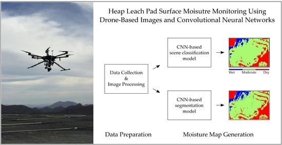
Graphical Abstract

1. Introduction

Heap leaching (HL) is a hydrometallurgical technology that has been widely adopted by the mining industry in recent years due to its easy implementation and high economic feasibility for metal and mineral extraction from low-grade ore deposits [1]. In an HL operation, metal-bearing ore is piled on an impermeable pad (i.e., an engineered liner), and a water-based lixiviant (or leaching reagent) is irrigated on top of the heap surface [2]. The leach solution, driven by gravity, flows through the rock pile and contact with the ore, such that the metal or mineral of interest is extracted from the rock and dissolved into the solution [3]. The solution exits the base of the heap through slotted pipes and a gravel drainage layer located above the liner [2]. The metal-bearing pregnant leach solution (PLS) is collected in the PLS pond (commonly called pregnant pond) and then pumped to the processing facility for recovery of the extracted metal [1,2]. After the valuable metal is recovered from the PLS, the barren leach solution is pumped to the barren solution pond and reapplied to the heap surface after refortifying with lixiviant chemicals [2,4].
In the leaching process, a high ore recovery requires an even lixiviant coverage over the surface of the heap leach pad (HLP, the facility that contains the ore material) because a non-uniform distribution of surface moisture can lead to suboptimal leaching conditions, which may further result in operational challenges [2,5,6,7,8]. As HL is a continuously ongoing operation, monitoring plays a critical role in optimizing the production process and providing feedback to mine managers and decision-makers. The current practices of HLP surface moisture inspection are often performed by naked-eye observation and manual sampling, which are time-consuming, discontinuous, and intermittent. Moreover, the manual inspection is labor-intensive and can frequently expose technical personnel to the hazardous leaching reagent (e.g., dilute cyanide solution in gold leaching) [9].
There are limited efforts made in HL operations to develop practical tools for streamlining the surface moisture monitoring workflow and detecting operational issues, such as surface ponding of leaching reagent, defects of irrigation units (e.g., sprinklers or drip emitters), and poor compliance between the actual solution application pattern and the designed irrigation pattern. This raises a necessity to develop efficient and on-demand HLP monitoring methods. To achieve this goal, we present a practical framework for HLP surface moisture monitoring, starting with drone-based aerial image collection, followed by surface moisture map generation using convolutional neural networks (CNNs).
In recent years, data acquisition using drones (or unmanned aerial vehicles, UAVs) together with digital imaging sensors has been applied in various mining and geology projects [10,11,12,13]. The usefulness of UAVs for geological surveys have been proved by the ever increasing use of drones in outcrop mapping [14], post-earthquake monitoring [15], magnetic anomalies detection [16], and geological features annotation and identification [17,18], just to name a few. In addition to geological surveys, numerous studies and applications have demonstrated the practicality and effectiveness of employing UAVs in mining environments to perform surveying and monitoring tasks, including dust monitoring [19,20], blasting process monitoring [21], haul road monitoring [22], rock fragmentation analysis [23], and structural pit wall mapping [24,25]. However, to the best of our knowledge, the use of UAVs and sensing technology to perform HLP surface moisture monitoring has not been widely adopted, except that a few recent studies showcased the feasibility of using UAVs equipped with thermal infrared sensors for moisture monitoring [26,27]. In this paper, we present a case study of a UAV equipped with a dual gimbal system which allowed mounting a visible-light camera and a thermal infrared sensor on the drone to acquire aerial images. The high-resolution aerial sensing data was then processed through digital photogrammetry methods and CNNs to produce surface moisture maps, which visually depict the different moisture zones across the HLP surface.
Over the past several years, many studies and applications (e.g., agricultur, and forestry) utilized remote sensing and CNNs to conduct surface moisture recognition and monitoring tasks [28,29,30,31,32,33]. For instance, Sobayo et al. [28] employed a CNN-based regression model to generate soil moisture estimates using UAV-based thermal images acquired over farm areas; Ge et al. [31] adopted a CNN model with 1-D convolutions to estimate soil moisture on a global scale, based on four sources of satellite data; Wang et al. [34] collected soil echoes using an ultra-wideband radar sensor over a bare soil field and used two CNNs to classify the moisture levels associated with the different soil echoes patterns; and Isikdogan et al. [33] proposed a CNN, named DeepWaterMap, to generate surface water maps on a global scale (e.g., continential scale) based on satellite imagery.
A number of factors are contributing to make CNNs popular and applicable in a wide variety of application domains. First, CNNs are a particular type of neural network that typically consists of multiple layers, which have the ability to extract hierarchical features from the model input [35,36]. Layers that are close to the input can extract low- and mid-level features, while later layers can learn high-level (i.e., more abstract and semantically meaningful) feature representations [37]. Such a feature extraction ability allows predictive CNN models to exploit spatial and/or temporal correlations in the data when making predictions. The extracted features at different layers of the networks are learned automatically from the data through the training process [38,39]. There is no hand-engineered feature required, which improves the models’ generalization ability when applied to data within the same problem domain but previously not observed by the models [39,40,41]. When CNNs are used to process image data, they are often robust against challenging image conditions, including complex background, different resolution, illumination variation, and orientation changes [42].
The abovementioned characteristics contribute to the popularity of CNNs to process data with a grid-like topology (e.g., images, and videos) and make them suitable for tasks like scene classification and semantic segmentation (also known as pixel-wise image classification) [39,43]. In remote sensing, scene classification is referred to as categorizing a scene image into one of several predefined classes [44,45,46]. The scene images are often local image patches (or image blocks) extracted from one or multiple large-scale remote sensing images [47]. In contrast, semantic segmentation is referred to as assigning a semantic class to every pixel of an input image [38,43], and it is a natural step towards fine-grained inference after scene classification [48,49]. In this work, two CNN-based approaches for generating HLP surface moisture maps are presented, including a scene classification model, and a semantic segmentation network.
Overall, this article aims to showcase a thorough case study, presenting the experimental procedures, implementation details, and the generated outputs of the proposed surface moisture monitoring workflow. Field data collection was conducted over a gold HLP, and data analysis was performed off-line. The following sections elaborate our methodology for the UAV-based data acquisition and the moisture map generation process. Illustrations of the experimental results are included which is followed by a discussion on the advantages, limitations, and possible improvement of the proposed method.

2. Materials and Methods

2.1. Study Site

The study site is a sprinkler-irrigated HLP at the McEwen Mining’s El Gallo mine (25°38′ N, 107°49′ W), located in Sinaloa State, Mexico, approximately 100 km northwest of Culiacan, and 350 km northwest of Mazatlán (Figure 1a). The mine site resided in the Lower Volcanic Series of the Sierra Madre Occidental, dominated by rocks of andesitic composition [50]. The mineralization is hosted within a northeast structural trend with numerous sub-structures (e.g., breccia, and quartz stockwork) [21]. Gold is the primary metal produced, and heap leaching is used to extract the metal from the crushed ores. The HLP was constituted of multiple lifts, where the designed lift height was 10 m, and the maximum heap height was 80 m. The HLP had a footprint of approximately 22 hectares and was located north of the mine site [26]. The HLP material was crushed gold-bearing rock with an 80% passing particle size (P80) of 8 to 10 mm [26]. The HLP’s irrigation system had an average sprinkler spacing of 3 m, and a dilute cyanide solution was applied continuously at an average irrigation rate of 8 L/h/m2 during the field experiment.

2.2. UAV Platform and Sensors

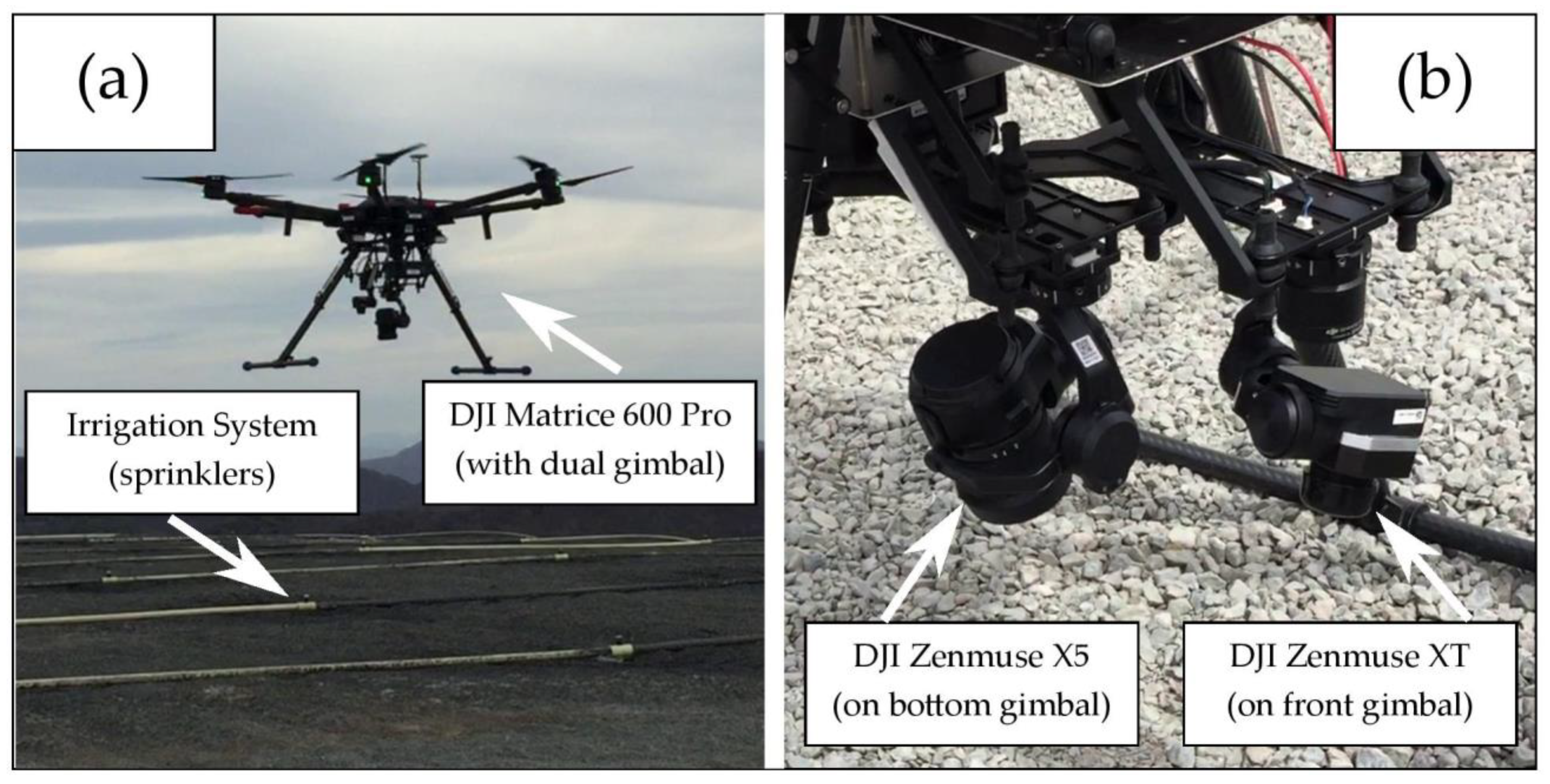
During the field data collection, a DJI Matrice 600 Pro hexa-copter (DJI, Shenzhen, China) was equipped with one visible-light (RGB) camera, DJI Zenmuse X5 (DJI, Shenzhen, China), and one thermal infrared (TIR) sensor, DJI Zenmuse XT 13 mm (FLIR Systems, Wilsonville, OR, USA) in a dual gimbal setup to acquire aerial images (Figure 2). The dual gimbal was a custom-built system, consisting of a front gimbal installed with a global positioning system (GPS) and a bottom gimbal without a GPS. This dual gimbal setup enabled the acquisition of both RGB and thermal images simultaneously. The RGB camera is a 16-megapixel camera with a maximum resolution of 4608 × 3456 pixels, and it was paired with a DJI 15 mm f/1.7 ASPH lens, which had a 72° field of view (FOV). This camera has a dimension of 120 mm × 135 mm × 140 mm and a mass of 530 g. The TIR sensor has a FOV of 45° × 37° and can capture electromagnetic (EM) radiation with wavelength ranging from 7.5 to 13.5 μm. The focal length of the TIR sensor is 13 mm, and the thermal images acquired have a resolution of 640 × 512 pixels. The TIR sensor has a dimension of 103 mm × 74 mm × 102 mm and a mass of 270 g. The UAV platform was selected because of its high payload capacity and versatile payload configuration. The two imaging sensors were selected because of their easy integration with the dual gimbal system, and more importantly, their suitability for conducting aerial remote sensing surveys [21,51,52,53].

2.3. Data Acquisition and UAV Flight Plans

From March 6th to 8th, 2019, field experiment and data acquisition were conducted over the HLP at the El Gallo mine. Two data collection campaigns were conducted in each surveying day, resulting in six campaigns in total throughout the field experiment. For each surveying day, the first data collection campaign was carried out in the morning (10 a.m.), and the second was in the afternoon (2 p.m.). This survey agenda was made to follow the mine site’s shift schedules and safety policies. During each data collection campaign, two flight missions were performed, where the first flight mission covered the top two lifts of the HLP, and the second covered the entire HLP surface (Figure 1b). The second mission was flown immediately after the completion of the first mission, and the total flight time for two missions together was approximately 30 min.
To generate flight plans for the two flight missions, the guidelines and practices described by Tziavou et al. [54] and Bamford et al. [21] were employed in this study. Several factors should be considered to create a flight plan for photogrammetry data collection, including image overlaps, target distance, and the sensors’ resolution, focal length, and field of view [21]. In this study, the data collection was performed by observing the HLP from a top-down view (i.e., the imaging sensors were tilted down to the nadir), and the distance between the HLP surface and UAV system was considered the main controllable parameter. To determine an appropriate flight altitude with respect to the HLP surface, the first step was to decide the objective ground sampling distance (GSD). The GSD is defined as the ground distance covered between two adjacent pixel centers of an image. In this study, the sprinkler spacing over the HLP was 3 m, and it was aimed to capture information with a spatial resolution finer than the sprinkler spacing. Bamford et al. [21] suggested that the objective GSD should be at least an order of magnitude smaller than the target dimension (i.e., 3 m in this case). Therefore, a GSD of approximately 10 to 15 cm/pixel was adopted for the field experiment. After determining the objective GSD, the required flight altitude was calculated as
z = GSD 2 i w i h 4 tan ( f h 2 ) tan ( f v 2 )
where iw and ih are the image width and height in pixels, respectively; fv and fh are the lens vertical and horizontal angle of view, respectively; GSD is the ground sampling distance in meters per pixel; and z is the flight altitude in meters [21,55]. Since the images taken by the TIR sensor had a lower spatial resolution than the ones taken by the RGB camera at the same flight altitude, the TIR sensor’s FOV and image size were used to design the flight plans. In this way, the range of flight altitude for the UAV system to achieve a GSD of 10 to 15 cm/pixel in the thermal images was 80 to 120 m. Once the fight altitude was determined, the detailed flight plans (e.g., flight lines, flight velocity, and flight duration) for image collection were automatically generated using the DJI Ground Station Pro application (DJI GS Pro) by inputting the flight altitude, the desired image overlaps, and a polygon of the area of interest to the application. In this study, the front and side overlaps for the thermal images were designed to be 85% and 70%, respectively, and the corresponding front and side overlaps for the RGB images were both approximately 80%. The details of the flight plans are summarized in Table 1 [26].
In each UAV data collection campaign, the following setup was used to collect the aerial images. The RGB camera was mounted on the UAV’s bottom gimbal, and the TIR sensor was attached to the front gimbal. The RGB and TIR sensors were operated using the DJI GS Pro and DJI GO applications, respectively, where both sensors were tilted down 90° to observe the HLP surface from a top-down view. The shutter intervals (i.e., the time between taking images) were set to five seconds per RGB image and two seconds per thermal image. The RGB images were saved in JPEG format, and the thermal image format was set to R-JPEG (radiometric JPEG). By the end of the field experiment, 24 sets of data were collected, which contained approximately 4750 thermal images and 2115 RGB images. Half of the datasets were for the whole HLP, and the other half were collected for the top two lifts of the HLP. Table 2 summarizes the number of data collected at each flight mission, where the thermal and RGB data are reported separately. It is worth mentioning that the front gimbal was installed with a GPS so that the GPS time synchronization between the drone and the TIR sensor resulted in georeferenced thermal images, whereas the RGB images were not georeferenced by the time of data collection because the bottom gimbal was not paired with a GPS device. Therefore, it was necessary to locate ground control points (GCPs) within the study area to help obtain positioning information. A GCP is an object with known real-world coordinates that can be identified in the collected images [56]. In this study, 12 GCPs were placed within the study area, and their locations were decided according to the accessibility over the HLP. The GPS coordinates of the GCPs were recorded using a portable GPS device prior to the first data collection campaign. The same 12 GCPs were used throughout the field experiment, and the locations of the GCPs are indicated in Figure 1b.

2.4. Image Processing

Image processing was conducted off-line after collecting data from the field experiment. A data preprocessing step was first performed for the RGB and thermal datasets. For the 12 RGB image sets, the corrupted and inappropriately exposed images were manually removed from the dataset. In total 4 out of 2114 RGB images were removed. The RGB images that cover one or multiple GCPs within the field of view were recorded manually so that the GPS coordinates of the GCPs could be used to geo-reference the images in the later steps. For the 12 thermal image sets, the poor-quality images were first removed by manual inspection, resulting in a removal of 47 out of 4748 images from the dataset. Then, an intensity transformation and mapping step was performed over the thermal images [26]. The FLIR Atlas SDK for MATLAB was used to extract the digital temperature value at each pixel location of the thermal images. The highest and lowest temperature values (denoted as Tmax and Tmin, respectively) within each of the 12 thermal image sets were then determined. Thus, 12 pairs of Tmax and Tmin were determined, where each pair corresponded to one of the thermal image sets [26]. Afterwards, the intensity value at each pixel location of the thermal images was mapped as
I x , y ( j ) = r o u n d ( T x , y ( j ) T min T max T min × 255 )
where round(∙) denotes the rounding function, which returns an integer intensity value within the range of 0 to 255 (i.e., 8-bit); T x , y ( j ) is the surface temperature in degree Celsius at the (x,y) pixel location of the jth image in the current image set; Tmax and Tmin are the highest and lowest temperature values in degree Celsius of the current image set; and I x , y ( j ) is the mapped pixel intensity value at the (x,y) pixel location of the jth image [26]. The above process was applied to each of the 12 thermal image sets independently, to generate 12 sets of grayscale images with the same number of images as the thermal image sets.
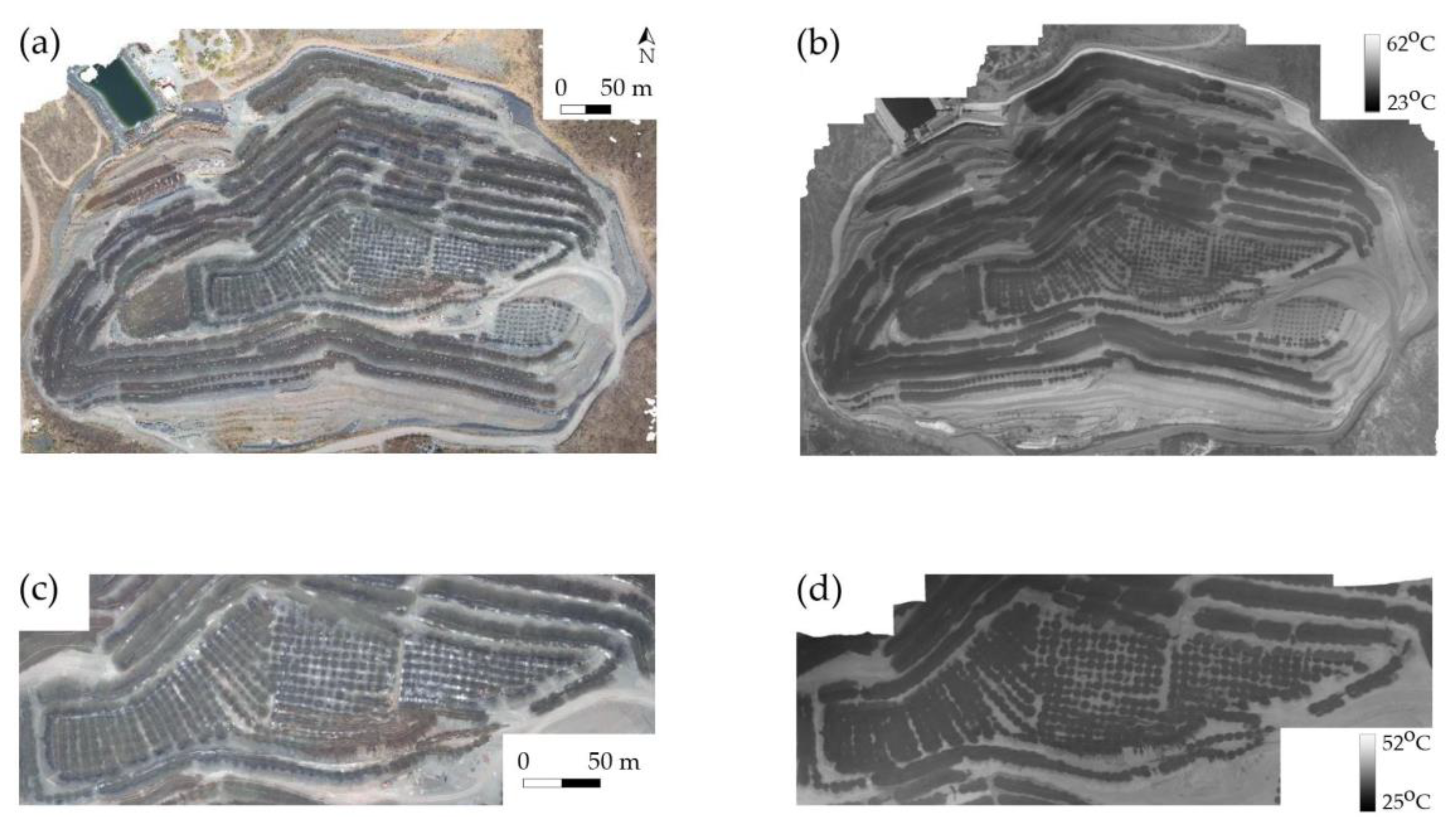
After completing the data preprocessing step, orthomosaics were generated in the Agisoft Metashape Professional software [57] using the preprocessed images. For the RGB image sets, the orthomosaic generation process started with importing the images into the software. Since the RGB images were not georeferenced, the images were not automatically registered after importation. Therefore, the GCP locations were manually pinpointed within the software interface, and the corresponding GPS coordinates were inputted into the software. The RGB orthomosaics were then generated using the Structure from Motion (SfM) workflow of the software, and this process was repeated using the same software settings for the 12 RGB image sets. For the thermal image sets, since the images were georeferenced during the data acquisition, they were automatically registered based on their georeference information after importation. The GCP coordinates were also used in this case mainly to refine the precision of image alignments. The SfM workflow was then used to generate the thermal orthomosaics. Figure 3a,c depicts examples of the generated RGB orthomosaics for the whole HLP and the two upper lifts.
Overall, 12 RGB and 12 thermal orthomosaics were generated, where half of these orthomosaics correspond to the whole HLP, and the other half are related to the top two lifts of the HLP. The generated RGB orthomosaics have a GSD of 2 cm/pixel and are in 24-bit image format (8-bit for each red, green, and blue channel), while the thermal orthomosaics have a GSD of approximately 10 cm/pixel and are in 8-bit image format (i.e., single-channel grayscale). The pixel intensity values of the thermal orthomosaics were converted to digital temperatures using the “Raster Calculator” function in the open source QGIS software (Version 3.4). The temperature value at each pixel location of a thermal orthomosaic was calculated as
T x , y = T min + ( T max T min ) I x , y I min I max I min
where I x , y is the pixel intensity value at the (x,y) pixel location of the thermal orthomosaic; Imax and Imin are the highest and lowest pixel intensity values, respectively; Tmax and Tmin are the highest and lowest temperature values in degree Celsius of the corresponding thermal image set; and T x , y is the converted temperature value in degree Celsius at the (x,y) pixel location of the thermal orthomosaic [26]. This process resulted in 12 surface temperature maps of the HLP, each map corresponded to one of the 12 thermal image sets (see Figure 3b,d for examples of generated temperature maps).
At this point, the 24 sets of images have been converted into 12 RGB orthomosaics and 12 temperature maps. Each orthomosaic was paired with one temperature map according to the region of interest and data acquisition time (Table 2). The next task was to superimpose the RGB orthomosaics over their corresponding temperature maps to produce 12 four-channel orthomosaics, where the first three channels contain the intensity values for the red, green, and blue colors, and the fourth channel containing the temperature information. The process of overlaying two images of the same scene with geometric precision is known as co-registration [58]. The co-registration process was achieved in three steps using the QGIS software. First, each pair of orthomosaic and temperature map was imported into the software, and the “Georeferencer” function was used to position the two images to the same spatial context. Since the RGB orthomosaics had a finer spatial resolution (GSD of 2 cm/pixel) than the temperature maps, the “Align Raster” function was then used to down-sample the RGB orthomosaic to achieve the same spatial resolution as the temperature map (GSD of 10 cm/pixel). The last step was to combine the two aligned images by “Merge” function in QGIS to generate the four-channel orthomosaic, where the data values in all four channels were single-precision floating-point numbers.

2.5. Dataset Creation and Partition for Moisture Map Generation Using CNN

In order to utilize the four-channel orthomosaics for HLP surface moisture mapping, two convolutional neural network (CNN) approaches were used. The first approach formulated the moisture map generation process as a scene classification task, while the second approach set up the process as a semantic segmentation problem. The CNN models employed in these two methods require different training, validation, and testing data, thus, the classification and segmentation datasets were prepared separately using the generated four-channel orthomosaics.
Overall, the dataset creation process comprises three steps. The first step was to subdivide the 12 four-channel orthomosaics into a number of non-overlapping image patches (or image blocks) such that each patch covers a small area of the HLP surface. Secondly, the small image patches were partitioned into training, validation, and test sets, which would be used in the CNN training and evaluation processes. Lastly, an image annotation step was performed to label all the examples (i.e., the image patches) so that the labelled examples can be used to train the networks in a supervised learning manner.

2.5.1. Creation of Scene Classification Dataset

To prepare the classification dataset, the 12 four-channel orthomosaics were first subdivided into a set of non-overlapping image patches with a size of 32 × 32 × 4 (height × width × channel) in the QGIS software. The image patches that covered areas outside the HLP were manually removed. In total 125,252 image patches were created. The image size of 32 × 32 pixels was used because this is one of the commonly used image resolutions in practice for the scene classification task [32,59,60]. Moreover, since the images had a GSD of 10 cm/pixel, every image patch represented approximately a 3.2 m by 3.2 m area on the HLP surface, which matched with the sprinkler spacing of the HLP’s irrigation system. The image patches related to the last data collection campaign (i.e., March 8, afternoon) were grouped as the held-out test set, for the model evaluation. The image patches from the other 11 data collection campaigns were then shuffled randomly and partitioned into the training set and validation set. Thus, the classification dataset is composed of a training set of 84,528 image patches (~70%), a validation set containing 20,008 image patches (~15%), and a test set with 20,716 image patches (~15%).
In this study, the classification model was expected to predict the moisture of the ground area covered by an input image patch. The predicted moisture condition should be given in one of the three classes, namely, “wet”, “moderate”, and “dry”. In other words, the models were trained to learn the correlation between pixel values and moisture levels and return a class estimate that best describes the moisture condition of a given area on the HLP surface. Therefore, each classification example was annotated with one of the three moisture classes. To annotate a classification example, a moisture estimation equation developed by the authors [26] was applied over the temperature channel, and the moisture value at each pixel location was calculated as
ω = 0.5103 ( T x , y ) + 23.77
where T x , y is the temperature value in degree Celsius at the (x,y) pixel location; and ω is the estimated HLP surface material gravimetric moisture content (%). The steps taken to develop the equation are elaborated in [26]. In short, Equation (4) was derived using linear regression based on 30 ground samples collected from the HLP. During each data collection campaign, five ground samples were collected. Care was taken during the sampling process to collect only the surface material (top 5–10 cm). The collected samples were sent to the on-site laboratory to measure their gravimetric moisture content. The sampling points were pinpointed within the acquired thermal images, and the temperature values at these locations were determined. Equation (4) was then derived through linear regression using the digital temperature values of the sampling locations as the independent variable and the measured moisture content of the ground samples as the dependent variable. The linear regression resulted in an R2 of 0.74 and a root mean square error (RMSE) of 1.28%, which demonstrated a good agreement between the predicted and measured moisture contents of the collected samples [26]. Using Equation (4), a mean value of moisture content for each classification example was calculated, followed by a thresholding operation. In this study, the “wet” class was defined as a moisture content greater than 8%, the “dry” class was defined as a moisture content smaller than 4%, and “moderate” class was for any moisture value falling within the range of 4% to 8%. These thresholds were defined based on site-specific operational practice and material properties. In this way, every classification example (i.e., image patch) was annotated by a moisture class, which indicated its moisture condition. Table 3 summarizes the frequencies and percentages of each moisture class in the classification dataset. It is important to note that different number of classes and moisture ranges can be considered for other heap leach sites.

2.5.2. Creation of Semantic Segmentation Dataset

Similar to the classification dataset, the preparation of the segmentation dataset started with splitting the 12 four-channel orthomosaics into a set of non-overlapping image patches. The image size was set to 64 × 64 pixels (height × width), resulting in the creation of 31,313 image patches in total. The image patches associated with the last data acquisition campaign (i.e., March 8, afternoon) were grouped as the held-out test set, and the remainder of the image patches was partitioned into the training and validation sets stochastically. Thus, the portions of the training set (21,132 examples), validation set (5002 examples), and test set (5179 examples) achieved an approximately 70/15/15 split of the data. In the semantic segmentation setup, the model was expected to classify every pixel of a given image into one of the three moisture classes (i.e., “wet”, “moderate”, and “dry”). A pixel-wise classification is used in the semantic segmentation [38,43]. The pixel-wise classification required the examples to be annotated at a pixel level. To annotate a segmentation example, Equation (4) was first applied to every pixel value in the temperature channel of the image patch. Subsequently, a pixel-wise thresholding operation was conducted to categorize the moisture values into one of the three moisture classes, with the same moisture content defined in the classification approach. The numbers “0”, “1”, and “2” were used to denote the “dry”, “moderate”, and “wet” classes, respectively. By following the above procedures, every segmentation example had its corresponding label image (or mask), and each mask was saved as a single-channel image with possible pixel values of “0”, “1”, and “2”. Table 4 summarizes the (pixel-level) percentage of each moisture class present in the dataset.
As shown in Table 3 and Table 4, it can be concluded that the majority of the data were labelled with a “moderate” moisture class, and the “wet” moisture class was a minority class in both the classification and segmentation datasets. The phenomenon of having skewed data distribution is called class imbalance, which naturally arises in many real-world datasets [43,61,62,63]. In this study, the data had an intrinsic imbalance; an imbalance created by naturally occurring frequencies of events rather than external factors like errors in data collection or handling [64]. The majority of the areas over the HLP surface were expected to have a moderate moisture condition, while the dry and wet areas should be minorities because the extreme moisture conditions may relate to operational issues. Several studies have shown that deep learning models can be successfully trained, regardless of class disproportion, as long as the data are representative [65]. It is also argued that the percentage of the minority becomes less influential if the minority class contains a sufficient number of examples [64]. In our case, the prepared datasets should be considered sufficient for training the CNNs because the number of training examples in the minority class (i.e., the “wet” moisture class) is already of the same size as the majority class of some benchmark datasets that have been extensively used in practice [59,64,66].

2.6. Scene Classification CNNs

This section introduces the network architectures and training setup of the three classification CNNs employed in this study. The three networks adopted for the experiment were AlexNet [67], ResNet [68], and MobileNetV2 [69], where several modifications over the network architectures were made to adapt for the prepared dataset. AlexNet was initially proposed by Krizhevsky et al. [67], which has revolutionized the field of computer vision and is one of the key contributors to the recent renaissance of neural networks [36]. AlexNet and its variants have been extensively used as baseline models in many research studies [34,36,70]. A modified version of AlexNet was adopted in this work to learn the correlation between the image input and the moisture class output. ResNet (or Residual Network) is a ground-breaking architecture proposed by He et al. [68] that has significantly improved the performance of CNNs in image processing and visual recognition tasks. The residual learning framework has been proved useful for training deep neural networks [37,71]. In this study a 50-layer ResNet (ResNet50) was used for the moisture classification task. The last network adopted was a modified version of MobileNetV2. This network was initially proposed by Sandler et al. [69], and is an efficient network particularly designed for resource-constrained computational devices (e.g., onboard computers) while preserving high prediction accuracy.

2.6.1. Network Architectures of Classification CNNs

The modified AlexNet implemented in our experiment contained eight layers with weights, where the first five layers were convolutional (Conv), and the reminders were three fully-connected (FC) layers. There were also two max pooling layers without weight involved in the architecture to down-sample the intermediate feature maps (also called activation maps). The architecture is summarized in Table 5.
The inputs to the network were image patches with a dimension of 32 × 32 × 4 (height × width × channel). All of the Conv layers in the network used 3 × 3 kernels with a stride of one. The first and the second layers did not use zero padding to adjust the layer’s input dimension, whereas the third to the fifth convolutional layers adopted a zero padding to ensure that the layer’s input and output had the same height and width. Max pooling layers with 2 × 2 non-overlapping windows and a stride of two were used to down-sample the feature maps such that the height and width became one half after each pooling operation. The last three layers were FC layers, where the first two had 1024 neurons (or hidden units) each, and the final layer was a three-way FC layer with softmax. The final output of the network was a 3 × 1 vector, containing the predicted probabilities for each of the three moisture classes. The ReLU activation function [72] was applied to all convolutional and fully-connected layers except for the output in which a softmax was used [67]. The whole network included 17.2 million trainable parameters.
For the ResNet50 architecture, the network comprised 50 layers with weights, including 49 Conv layers and one FC layer [68]. There was also one max pooling and one global average pooling layer, which did not have trainable weight. Batch normalization [73] was applied after every Conv layer, and the ReLU nonlinearity was used as the activation function except for the output layer. The architecture of ResNet50 is summarized in Table 6, and the final output of the network was a 3 × 1 vector containing the predicted probabilities for each of the three moisture classes. In Table 6, each square bracket in the third column represents a bottleneck residual block, and every row in the brackets denotes one layer of operation. The inner structure of a bottleneck residual block is illustrated in Figure 4a [68]. Every bottleneck residual block consisted of three layers: a 1 × 1 Conv layer [74] for dimension reduction, a 3 × 3 Conv layer of regular convolution, and a 1 × 1 Conv layer for dimension restoration [75]. Moreover, the bottleneck residual block included a shortcut connection that skipped the Conv layers and performed an identity mapping. One copy of the input first propagated through the three stacked convolutional layers, followed by adding another copy of the input from the shortcut to generate the block output [75]. The use of bottleneck residual blocks leads to an effective and computationally efficient training process of ResNet50 [68]. Overall, the whole network had 23.6 million parameters, including 23.5 million trainable and 53 thousand non-trainable parameters.
In this study, a modified version of MobileNetV2 [69] was implemented, and the network architecture is summarized in Table 7. The model took image patches with a dimension of 32 × 32 × 4 (height × width × channel) as input, and outputted a 3 × 1 vector containing the predicted probabilities for each of the three moisture classes. The network started with a regular 3 × 3 Conv layer with 32 filters, followed by six inverted residual blocks, and ended with a global average pooling, a three-way FC layer, and a softmax. In Table 7, each square bracket in the third column represents an inverted residual block, and every row in the brackets denotes one layer of operation. In general, an inverted residual block appears similar to the building block of ResNet (i.e., Figure 4a), except that the shortcut connection directly occurs between bottleneck layers rather than feature maps that have a high number of channels [69]. The reduction in the number of channels for the block outputs can be seen by comparing the second column of Table 6 and Table 7. Moreover, the inverted residual blocks replace regular convolution with depth-wise convolution (Dwise Conv) [76] to reduce the number of multiply-adds calculations and model parameters [69]. The extensive use of inverted residual blocks in concert with Dwise Conv layers in MobileNetV2, significantly lessens its memory footprint and computational burden, resulting in a highly efficient network [69]. It is worth noting that the inverted residual blocks with different stride values had different inner structures. For “Block1” to “Block5” in Table 7, the stride of each block is provided in the last column of the table, and the corresponding inner structures are depicted in Figure 4. Overall, the network had 109 thousand parameters in total, which included 103 thousand trainable and 6 thousand non-trainable parameters.

2.6.2. Training Setup of Classification CNNs

All three architectures were implemented in TensorFlow 2 (TF) [77], and the network training was deployed using TensorFlow’s Keras API [78]. All networks were trained from scratch using RMSProp optimizer [79] with a learning rate of 0.001, a momentum of zero, and a decay (named rho in TF) of 0.9. There was no extra learning rate decay used during the training, and the cross-entropy loss (named sparse categorical cross-entropy in TF) was used as the loss function. The training data were normalized to have zero mean and unit standard deviation for every channel, and no data augmentation was performed during the training process. The validation and testing data were also normalized using the training set’s mean and standard deviation [68,80].
For the training of AlexNet, dropout [81] was applied to the first two FC layers with a dropout probability of 0.5, whereas there was no batch normalization (BN) used in the architecture [67]. In contrast, no dropout was used in ResNet50, but BN with a momentum of 0.99 was used after every convolution and before activation [68]. Similarly, no dropout was adopted for MobileNetV2, while BN with a momentum of 0.999 was applied after every convolutional operation, including regular, depth-wise, and 1 × 1 (also called pointwise [76]) convolutions [69].
To train a model, the training process started with initializing the network’s weights using the Kaiming initialization proposed by He et al. [82]. The model was then trained for 20 epochs with a minibatch size of 72 examples. It is worth noting that the training set contained 84,528 examples, which can be divided by 72 with no remainder so that each epoch consisted of 1174 steps (or iterations). In order to conduct a fair comparison regarding the performance of the three employed architectures, 30 copies of each network (i.e., 30 models for each architecture, 90 models in total) with different initialization of the network parameters were trained. After completing the 20 epochs of training, the trained models were examined against the validation set. Since different initialization for the weights of a network can lead to variations in the model performance, the one (out of 30 models with the same architecture) that resulted in the best prediction accuracy on the validation set was chosen to be the final model. Thus, three final models were determined (one for each architecture), and they were evaluated on the test set to compare the three architecture’s classification accuracy. All models were trained on a computer with an NVIDIA GeForce RTX 3090 graphical processing unit (GPU), AMD Ryzen 3950X central processing unit (CPU), and 128 GB of random access memory (RAM). The training time for 20 epochs of the modified AlexNet, ResNet50, and modified MobileNetV2 using the abovementioned training setup were approximately 6.5 min, 34 min, and 5 min, respectively.

2.7. Semantic Segmentation CNN

This section presents the network architecture and training setup of the semantic segmentation CNN employed in the experiment. A modified version of U-Net was used that had a typical encoder-decoder structure [83,84]. U-Net is a semantic segmentation CNN originally proposed by Ronneberger et al. [83]. The network architecture is comprised of two parts: the encoder part (also called contracting path or compression stage) that convolves an input image and gradually reduces the spatial size of the feature maps; and the decoder part (also called expansive path or decompression stage) that gradually recovers the spatial dimension of the intermediate features and produces an output segmentation map with the same or a similar height and width as the input [83,85]. The two parts of the network are more or less symmetric, and the network appears as a U shape, leading to the name of the architecture [83].

2.7.1. Network Architectures of Segmentation CNN

The network architecture of the implemented modified U-Net is summarized in Table 8. The encoder part of the network involved four encoder blocks, and each block consisted of two 3 × 3 convolutions (with a zero padding and a stride of one), each followed by a ReLU nonlinearity. The output of each encoder block had a doubled number of feature channels as the input, and the output of the last encoder block had 512 feature channels. The down-sampling between encoder blocks was performed using a 2 × 2 max pooling layer with a stride of two such that the height and width of the feature map were halved after the pooling operation (Table 8).
In the decoder part of the network, every preceding decoder block was connected to the succeeding one through an up-convolution (also called transposed convolution or sometimes deconvolution) that halved the number of channels and doubled the height and width of the feature map. Meanwhile, a skip connection was used to copy and concatenate the output of the corresponding encoder block to the up-sampled decoder feature map (i.e., the concatenate operations in Table 8). The concatenation of the feature maps helped the model learn to create well-localized hierarchical features and assemble precise output [83,86]. Within each decoder block, two 3 × 3 convolutions (with a zero padding and a stride of one) were included, followed by a ReLU nonlinearity after each convolution.
To generate the model output, a 1 × 1 convolution with softmax was used to map the 64-channel features to the final three-channel feature map, where each channel contained the predicted probabilities for the corresponding moisture class at each pixel (i.e., the first channel at a pixel contained the probability for the “dry” class, and the second and the third channels were for the “moderate” and “wet” classes, respectively). The single-channel segmentation map was then created by applying a pixel-wise Argmax operation over the three-channel feature such that the moisture class with the highest probability was used to represent the moisture condition at each pixel location. In total, the network had 7.7 million parameters, which were all trainable parameters.

2.7.2. Training Setup of Segmentation CNN

The modified U-Net architecture was implemented in TensorFlow 2 [77], and the networks were trained using the prepared segmentation dataset. All models were trained from scratch using RMSProp optimizer [79] with a learning rate of 0.001, a momentum of zero, and a decay of 0.9. Neither dropout nor batch normalization was applied in the network, and there was no extra learning rate decay used during the training. The training data were normalized to have zero mean and unit standard deviation for every channel, and the validation and test data were also normalized using the training set’s mean and standard deviation [68]. Similar to the classification case, 30 copies of the network were trained, where the parameters of the models were initialized differently using the Kaiming initialization method [82]. Each model was trained for 20 epochs with a minibatch size of 36 examples, and the cross-entropy loss was used as the loss function. The training time for 20 epochs was approximately 8.5 min for each model. After completing the training, the one model (out of 30) that returned the best performance on the validation set was selected to be evaluated against the test set.

2.8. Moisture Map Generation

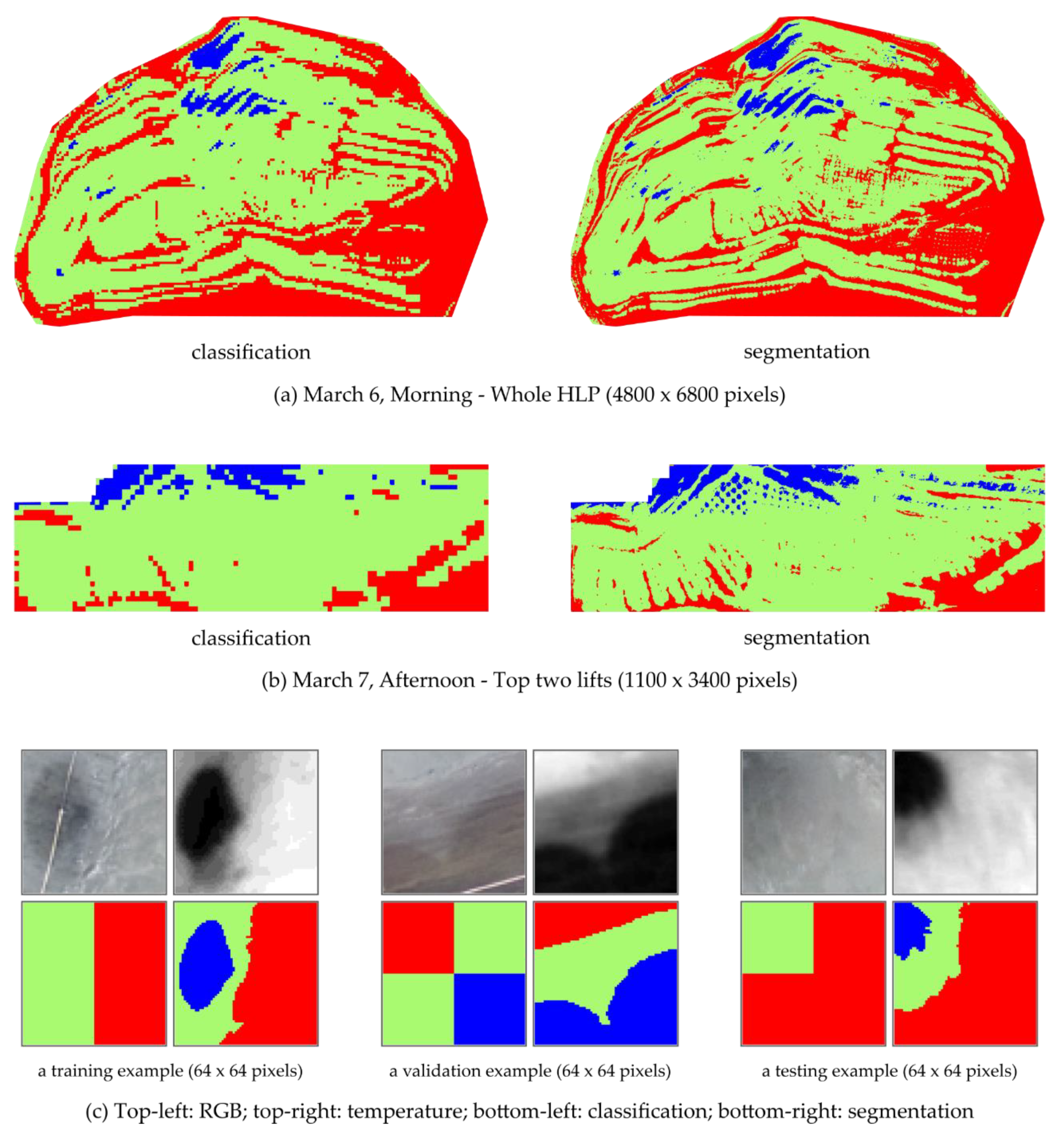
The moisture map generation pipeline of the two approaches is summarized in Figure 5. Overall, the workflow started with subdividing the input orthomosaic into multiple non-overlapping image patches with the same size (32 × 32 for classification and 64 × 64 for segmentation). These image patches were then used as input to the predictive CNN models to produce the corresponding prediction for each image patch. Finally, the model predictions were combined based on their initial positions in the input orthomosaic to create the moisture map output (Figure 5). For both approaches, the workflow’s input was the generated four-channel orthomosaics, where the first three channels were red, green, and blue channels, respectively, while the fourth was the temperature channel. All pixel values in the orthomosaics were floating-point numbers, and the intensity values in the color channels were within the range of 0 to 255 (inclusive). The values in the temperature channel had a unit of degree Celsius, and the digital numbers generally fell within the range of 10 to 70 in the prepared data.
For the classification approach, a trained CNN moisture classifier was utilized in the pipeline, and the input orthomosaic was split into non-overlapping image patches with a size of 32 × 32 pixels (height × width). The pixel values of the image patches were then normalized by subtracting the per-channel mean and dividing by the per-channel standard deviation of the (classification) training set. Afterwards, the CNN moisture classifier was used to assign a class to each image patch, and the image patches were color-coded based on the assigned moisture class (i.e., one color for all pixels in an image patch). The “wet”, “moderate”, and “dry” classes were denoted by a blue, greenish, and red color, respectively, as shown in Figure 5.
In the segmentation approach, the input orthomosaic was split into image patches with 64 × 64 pixels, and the modified U-Net model was used to create segmentation maps. The pixel values of the image patches were normalized by first subtracting the (segmentation) training set’s per-channel mean, and then dividing by the per-channel standard deviation. Since the segmentation model performed pixel-wise classification, every pixel in the image patches was assigned with one moisture class and color-coded with the corresponding color (Figure 5). The moisture map of the HLP surface was then generated by combining the individual segmentation maps based on their corresponding positions in the input orthomosaic.

3. Results

3.1. Evaluation of Classification CNN

The box plots in Figure 6 summarize the model performance of the trained CNN moisture classifiers on the validation set. As mentioned in Section 2.6.2, there were 30 models trained for each of the three network architectures, and each box plot in Figure 6 represents the distribution of prediction accuracy for the 30 models after 20 epochs of training. Two nonparametric statistical tests, namely two-sample Kolmogorov–Smirnov (KS) test and Wilcoxon rank-sum (WRS) test (also known as Wilcoxon–Mann–Whitney test), were conducted to assess whether there are significant differences among the three empirical distributions [87,88,89]. The statistical tests were carried out in a pair-wise manner (i.e., AlexNet to ResNet50, AlexNet to MobileNetV2, and ResNet50 to MobileNetV2), and the null hypothesis of each test states that the underlying distributions of classification accuracy on the validation set for the two architectures are identical [87,89]. As shown in Table 9, the statistical test results indicate that the modified AlexNet’s classification accuracy on the validation set may have a significant difference compared to the other two architectures because the null hypothesis was rejected at the 5% significance level in both KS and WRS tests. On the other hand, the null hypothesis was not rejected when comparing the ResNet50 to the modified MobileNetV2, indicating that there may be a distributional equivalence between the two distributions [87,88,89,90].
Overall, the models with all three architectures were able to converge and achieve a high accuracy (more than 92%) on the validation data. The ResNet50 and modified MobileNetV2 networks, on average, had a better performance than the modified AlexNet models given the training setup described in the previous section. Among the three architectures, the ResNet50 models had the broadest range of validation accuracy, and this variation in model performance reveals the inherent randomness and uncertainty involved in the model training process. The best classifiers of the modified AlexNet, ResNet50, and modified MobileNetV2 had a classification accuracy of 97.8%, 99.0%, and 98.7%, respectively, on the validation set. These three models, which resulted in the highest prediction accuracy among their architecture, were selected to evaluate against the test set (data of March 8, afternoon), and the results are summarized in Table 10.
As presented in Table 10, all three models achieved high overall accuracy on the test set (98.4% for modified AlexNet, 99.2% for ResNet50, and 99.1% for modified MobileNetV2). However, the modified AlexNet had the lowest true-positive rates (i.e., sensitivity or recall) for both the “dry” (98.8%) and “wet” (84.6%) examples among the three models, resulting in the highest miss rates (false-negative rate) for these two moisture classes. The high miss rate led to 15.4% of the “wet” examples predicted as the “moderate” moisture class, which implies that the model could overlook a considerable amount of overly irrigated area on the HLP surface if the model were used in practice. Both ResNet50 and MobileNetV2 models achieved similar performance on all three moisture classes, and the miss rate for the “wet” class was approximately one-fifth of the modified AlexNet model. In addition to the prediction accuracy, the inference time (with a batch size of one) of the modified MobileNetV2 was approximately one half of the ResNet50 in our experimental setup, and thus the modified MobileNetV2 model provided the best balance between classification accuracy and computational efficiency for our prepared data.

3.2. Evaluation of Segmentation CNN

To evaluate the performance of the modified U-Net models, two commonly used accuracy metrics for semantic segmentation, namely Global Accuracy (also called pixel accuracy, PA) and Mean Intersection over Union (MIoU), were adopted. Pixel accuracy is a simple metric that calculates the ratio between the number of correctly classified pixels and the total number of pixels [48,49]. The expression of PA is defined as
P A = i = 1 N cls n i i N pixel
where PA is the pixel accuracy expressed in percentage; N cls is the total number of classes, which is equal to three in this study for the three moisture classes; n i i denotes the number of pixels that are both predicted and labelled as the ith class (i.e., true positives, TP); and N pixel is the total number of pixels of the data [86]. The PA metric is commonly used due to its simplicity, but it is not always a good measure of the model performance when the dataset has a class imbalance issue. A model that consistently biases toward the majority class can still result in a relatively high pixel accuracy. In contrast, the Intersection over Union (IoU) metric takes the similarity and diversity of the predicted and labelled segmentation maps into account [86]. The expression of per-class IoU is defined as
I o U i = n i i j = 1 N cls n i j + j = 1 N cls n j i + n i i ,   i j
where N cls is the number of classes; subscript i and j are indices denoting different classes; I o U i is the intersection over union of the ith class in percentage; n i i is the true-positives with the same definition as in Equation (5); n i j is the number of pixels that are predicted as the ith class, but the true label is the jth class (i.e., false positives, FP); and n j i is the number of pixels that are predicted as the jth class, but the true label is the ith class (i.e., false negatives, FN) [86]. In short, the per-class IoU metric is the ratio between true positives (intersection) and the sum of TP, FP, and FN (union) for each class [49]. The MIoU metric is the class-averaged IoU defined as
M I o U = 1 N cls i = 1 N cls n i i j = 1 N cls n i j + j = 1 N cls n j i + n i i ,   i j
where all terms have the same definitions as in (6). In practice, MIoU is considered the standard metric for evaluating semantic segmentation techniques [48,49,86].
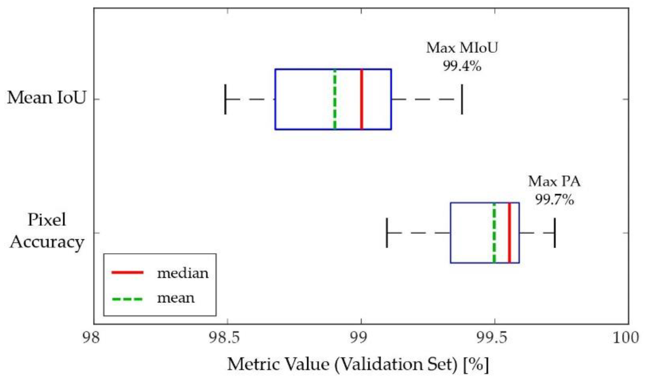
The model evaluation process started with computing the PA and MIoU metrics for the 30 trained models on the validation set. The one model that returned the highest sum of the two metrics was selected to be the final model, which was subsequently used to evaluate against the test set. Among the 30 trained networks, four models failed to converge, resulting in MIoU values less than 50% on both the training and validation data. For the remaining models that successfully converged, the box plots in Figure 7 summarize their performance on the validation set. A model that achieved a PA of 99.7% and an MIoU of 99.4% on the validation data was selected, and its performance on the test set is summarized in Table 11. The per-class F1 score (also known as the dice coefficient) metric shown in Table 11 is calculated as
F 1   s c o r e i = 2   ×   T P i   F P i   +   F N i   +   2   ×   T P i
where T P i , F P i , and F N i are the number of true positives, false positives, and false negatives, respectively, of the ith class as defined in Equation (6) [86]. Despite some segmentation errors are observed in the “wet” moisture class, the final model achieved similar performance on the test set compared to the validation set, and the model demonstrated a good competency and generalization ability in creating accurate segmentation maps based on our prepared data.

3.3. Generated HLP Surface Moisture Maps

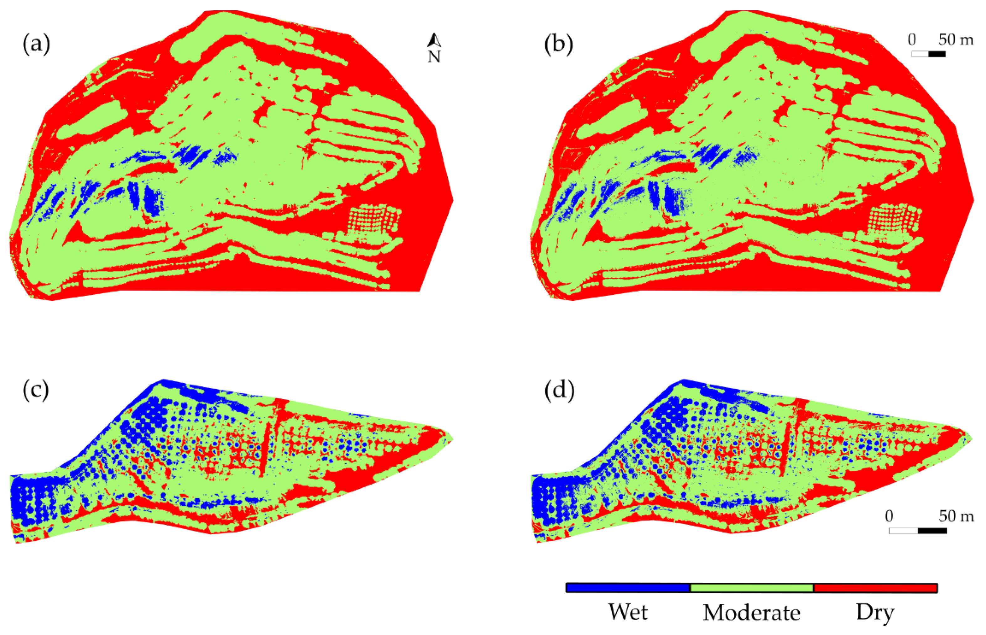
Figure 8 illustrates the generated moisture maps for the whole HLP based on the data collected on March 8 (afternoon) using the classification approach. The modified AlexNet, ResNet50, and modified MobileNetV2 classifiers produced comparable results against each other, and only minor differences were observed in the resultant outputs. The reference moisture map (Figure 8d) was created by following the same procedure used to prepare the training, validation, and testing data described in Section 2.5. Overall, the correlation between the input image patches and their corresponding moisture classes were effectively learned by the trained models, and the generated results provided a high-level overview of the moisture status across the HLP surface. Since the classification models only returned one prediction for each input, this implies that the moisture condition was assumed uniform within the area covered by each image patch. Such an assumption is acceptable if only an overview of a large study area is required. Nevertheless, some monitoring tasks in practice, such as pinpointing malfunctioning sprinklers, may require moisture maps with a fine resolution (e.g., sub-meter level). In order to generate moisture maps with higher resolution for depicting a fine-grained moisture distribution over the HLP, the segmentation approach was employed to perform pixel-wise moisture prediction for the input orthomosaics.
Figure 9 shows examples of the generated moisture maps using the segmentation approach. The results shown in Figure 9 demonstrate that the trained model effectively learned the pixel-wise mapping between the input image and the output segmentation maps. The generated moisture maps had the same GSD (10 cm/pixel) as the input orthomosaic, and a comparison between the outputs of the two approaches is provided in Figure 10. As shown in Figure 10a, both methods created moisture maps displaying the same moisture distribution pattern across the whole HLP surface. However, the distinction becomes apparent when the moisture variation of a relatively small region is depicted (Figure 10b,c. The produced results by the classification method appear pixelated, and the wetted area (or wetted radius) of each sprinkler is not noticeable in the classification case. In contrast, the segmentation moisture maps preserve fine-grained details, and the boundaries of different moisture zones are clearly outlined.
Despite the similarity and difference of the two approaches, the decision on which model to use may consider not only the amount of detail required from the generated output but also the amount of time and computational resources available for the application. Although the segmentation approach preserves fine-grained information in the produced results, segmentation networks may require longer training time, larger memory footprint, and sometimes have more model latency than classification CNN models. The computational burden can become a challenge if efficient data analysis is required or computational resource is limited (e.g., onboard computer).

4. Discussion

The results illustrated in Figure 8 and Figure 9 demonstrate the effectiveness of the described workflow for HLP surface moisture mapping using drone-based aerial images and convolutional neural networks. The use of UAV and sensing technology can improve data collection over HLPs, and the advanced computer vision and image processing techniques can bring values into the HLP monitoring process.
In general, there are several advantages of using UAV platforms equipped with imaging sensors to acquire data over HLPs. First, the use of UAVs for data collection increases the safety of personnel by reducing exposure to hazardous material (i.e., the leaching reagent). The regions inaccessible to humans over the HLPs (e.g., the side slopes of the HLP) can be observed by taking aerial images from top and oblique views. Furthermore, UAV-based data acquisition reduces time effort in data collection because a large area can be surveyed within a short time without disrupting ongoing production operations. When one or more imaging sensors are mounted on a UAV, the obtained images will become a permanent record of the field conditions at a specific point of time, which can be revisited in the future as required [21]. These permanent records are also beneficial for other monitoring tasks, such as design compliance audit and change detection. In addition, the remotely sensed data are generally with high spatial and temporal resolutions, which can not be achieved by manual point-measurement methods or even satellite-based approaches [91]. The high-quality aerial sensing data can be processed using digital photogrammetry programs, and the outputs can be co-registered with geometric precision to build multi-channel orthomosaics, which simultaneously contain information captured from different imaging sensors. The created orthomosaics can be further processed by CNNs to generated HLP surface moisture maps.
One significant advantage of CNNs is their ability to synchronously accommodating data with different modalities (e.g., data acquired from RGB camera and TIR sensor) while learning complex functions automatically without the need for feature engineering and variable selection [91]. In this study, all the classification and segmentation CNNs were capable of learning correlations between the four-channel input images and the corresponding output moisture classes. Most of the trained models manifested high prediction accuracy on the prepared dataset, and the adopted training scheme was effective for training the models to converge successfully. The two proposed approaches were both applicable to create moisture maps depicting the moisture distribution pattern of the whole HLP. The segmentation method can perform pixel-wise moisture prediction, preserving fine-grained information about the moisture variations. The generated moisture maps provide direct visualization of the different moisture zones on the HLP surface, and such information can be used in practice to monitor and improve the HL operations.
Overall, the generated moisture maps can be utilized to detect potential safety concerns and optimize the irrigation system of HL operations. In practice, excessive irrigation can lead to ponding or puddles of solution over the HLP surface, and the superabundant can potentially cause liquefaction, which can further result in catastrophic collapse or landslide of the HLP [27,92]. Moreover, solution ponds on the heap surface can become a threat to wildlife due to the toxicity of the leaching solution [93,94]. Therefore, the generated moisture maps can be used to show the over-irrigated zones, and operators can take timely measures to address the operational issues. In addition, the moisture maps can also help locate the dry areas, which are often related to an insufficient irrigation rate or defects of solution spreading devices (i.e., sprinklers in this study). Early detection of malfunctioning sprinklers can help technical staff descale or replace the irrigation units promptly, which can lead to an increase in production efficiency because dry areas may cause a loss of mineral recovery [92]. Furthermore, the moisture maps can be integrated into an automated irrigation system, where a controller can dynamically adjust the solution application rate at different regions according to their moisture status [27]. In such a setting, the irrigation rate can be automatically lowered for the wet zones to reduce lixiviant consumption, while a higher flow rate is sent to the dry areas to avoid a deficiency in solution application [27,92].
Despite the aforementioned benefits, there are limitations of the proposed method for HLP monitoring. Firstly, the use of UAVs in mining environments can be limited or restricted by regulations, and the regulatory requirements about flying drones can vary in different jurisdictions [21]. In addition, weather and environmental conditions have a significant impact on the data obtained by the UAV system. The variations of lighting conditions and cloud shadowing often have a large influence on the quality of images [26], especially for the data captured by RGB cameras. Cloud cover, for instance, can result in underexposed regions on the RGB images, which may add complexity to the data processing [21]. Similarly, the ever-changing meteorological and atmospheric conditions can affect the consistency of the measurements recorded by TIR sensors because the gasses and suspended particles can absorb, scatter, and emit radiation during the energy transfer process [26,95]. Moreover, current UAV platforms are generally not available to operate in extreme weather, such as rain, snow, and storm; also, consistently exposing a UAV system to a dusty and hot environment can damage the drone and wear the onboard sensors, resulting in reduced durability of the equipment [21]. Beyond the environmental conditions, several logistics factors ought to be considered during the field data collection. Generally, data acquisition using RGB cameras should be conducted in the day shift of the mine’s schedule because the lighting conditions during the afternoon and midnight shifts are often suboptimal for taking visible-light images for the HLP. Since the surveyor who is controlling the UAV during the flights should be an appropriately trained pilot, the time available for data acquisition can be constrained because each mine may only have a limited number of trained pilots. Therefore, a careful arrangement of the survey schedule is important, and effective communication between the pilot and the other members of the survey team is crucial in order to obtain the desired data.
To improve and extend the proposed workflow for HLP surface moisture monitoring, there are several aspects which may require further investigate. In this study, data acquisition was conducted at only one mine site during a three-day duration. Future studies should conduct more field experiments and collect more representative data to refine the proposed data collection and image analysis methods. It is worth noting that UAV-based data acquisition practices can vary significantly even for similar applications. Different researchers or practitioners may develop disparate practices through the learning-by-doing approach [96]. This can be attributed to the site-specific conditions in concert with the different combinations of drones and sensors which add flexibility and complexity to the survey planning and data acquisition process. Therefore, conducting field experiments and gradually refining the experimental procedures may be essential to develop a robust and effective drone-based surveying routine for HLP monitoring. For the image processing methods, the co-registration of the thermal and RGB orthomosaics was performed manually in this study. The manual image co-registration process was labor-intensive, and the resultant product was subject to reproducibility issues due to the extensive human intervention. A number of studies have proposed various area-based approaches (e.g., Fourier methods, and mutual information methods) and feature-based approaches (e.g., using image feature extractors combined with the random sample consensus algorithm to compute image transformation) to automate the co-registration of data with multimodality [43,97,98,99]. Future studies may incorporate and implement several of these algorithms to streamline the image processing for more efficient data analysis. The project’s ultimate goal should aim to develop a system capable of real-time and on-demand HLP surface moisture monitoring, and the data processing pipeline should move towards a fully-automated approach to minimize human intervention. Such improvement can increase the reproductivity of the generated results as well as reduce time efforts required for data processing. In addition to the automation of the monitoring procedures, future studies may explore the feasibility of using UAV systems to collect multispectral or hyperspectral data for various monitoring tasks because the remote sensing data captured in different electromagnetic wavelengths can reveal different properties of the HLP material. This research direction will result in a new set of data analytics methods, which will complement the proposed framework in this study.

5. Conclusions

This article presented a thorough case study of using drone-based aerial images and convolutional neural networks for HLP surface moisture monitoring. The presented workflow started with acquiring RGB and thermal images by equipping a UAV with one visible-light camera and one thermal infrared sensor. The collected aerial data were processed through digital photogrammetry and convolutional neural networks, and the generated results provided direct visualization of the different moisture contents across the HLP surface. Two CNN-based moisture generation approaches were proposed, where the first approach utilized a scene classification setup, and the second formulated the process as a semantic segmentation task. Methodology and implementation details were elaborated throughout the paper, and the advantages, limitations, and possible future improvements of the presented method were discussed. The results from the experiments and data analysis demonstrate that drone-based data collection can provide safe, continuous, on-demand, and fast acquisition of high-quality data, while the generated surface moisture maps can facilitate timely decision making and increase the efficiency in detecting and resolving potential operational issues in HL operations. Future work will devote to developing more automated systems to decrease the amount of human intervention required to complete analysis and exploring the feasibility of using other combinations of onboard sensors to acquire information from HLPs.

Author Contributions

Conceptualization, M.T. and K.E.; methodology, M.T. and K.E.; software, M.T.; validation, M.T. and K.E.; formal analysis, M.T. and K.E.; investigation, M.T. and K.E.; resources, K.E.; data curation, M.T. and K.E.; writing—original draft preparation, M.T.; writing—review and editing, K.E.; visualization, M.T.; supervision, K.E.; project administration, K.E.; funding acquisition, K.E. All authors have read and agreed to the published version of the manuscript.

Funding

This research was funded by Natural Science and Engineering Research Council of Canada (NSERC), grant number CRD-PJ-508741-17.

Institutional Review Board Statement

Not applicable.

Informed Consent Statement

Not applicable.

Data Availability Statement

The data used for the model development are available from the corresponding author upon reasonable request and permission from the industry partner.

Acknowledgments

The authors would like to thank McEwen Mining Inc. for their financial and technical support and Vector Institute for Artificial Intelligence for their technical support. Furthermore, the authors would like to thank Thomas Bamford and Filip Medinac for assisting the field experiment.

Conflicts of Interest

The authors declare no conflict of interest. The funders had no role in the design of the study; in the collection, analyses, or interpretation of data; in the writing of the manuscript, or in the decision to publish the results.

References

  1. Ghorbani, Y.; Franzidis, J.-P.; Petersen, J. Heap leaching technology—Current state, innovations, and future directions: A review. Miner. Process. Extr. Met. Rev. 2016, 37, 73–119. [Google Scholar] [CrossRef] [Green Version]
  2. Pyper, R.; Seal, T.; Uhrie, J.L.; Miller, G.C. Dump and Heap Leaching. In SME Mineral Processing and Extractive Metallurgy Handbook; Dunne, R.C., Kawatra, S.K., Young, C.A., Eds.; Society for Mining, Metallurgy, and Exploration: Englewood, CO, USA, 2019; pp. 1207–1224. [Google Scholar]
  3. Kappes, D.W. Precious Metal Heap Leach Design and Practice. In Mineral Processing Plant Design, Practice, and Control 1; Society for Mining, Metallurgy, and Exploration: Englewood, CO, USA, 2002; pp. 1606–1630. [Google Scholar]
  4. Watling, H. The bioleaching of sulphide minerals with emphasis on copper sulphides—A review. Hydrometallurgy 2006, 84, 81–108. [Google Scholar] [CrossRef]
  5. Lankenau, A.W.; Lake, J.L. Process for Heap Leaching Ores. U.S. Patent 3,777,004A, 4 December 1973. [Google Scholar]
  6. Roman, R.J.; Poruk, J.U. Engineering the Irrigation System for a Heap Leach Operation; Society for Mining, Metallurgy and Exploration: Englewood, CO, USA, 1996; pp. 96–116. [Google Scholar]
  7. Marsden, J.; Todd, L.; Moritz, R. Effect of Lift Height, Overall Heap Height and Climate on Heap Leaching Efficiency; Society for Mining, Metallurgy and Exploration: Englewood, CO, USA, 1995. [Google Scholar]
  8. Bouffard, S.C.; Dixon, D.G. Investigative study into the hydrodynamics of heap leaching processes. Met. Mater. Trans. B 2000, 32, 763–776. [Google Scholar] [CrossRef] [Green Version]
  9. Pyke, P.D. Operations of a Small Heap Leach; The Australasian Institute of Mining and Metallurgy: Victoria, Australia, 1994; pp. 103–110. [Google Scholar]
  10. Salvini, R.; Mastrorocco, G.; Seddaiu, M.; Rossi, D.; Vanneschi, C. The use of an unmanned aerial vehicle for fracture mapping within a marble quarry (Carrara, Italy): Photogrammetry and discrete fracture network modelling. Geomatics Nat. Hazards Risk 2016, 8, 34–52. [Google Scholar] [CrossRef]
  11. Valencia, J.; Battulwar, R.; Naghadehi, M.Z.; Sattarvand, J. Enhancement of explosive energy distribution using UAVs and machine learning. In Mining Goes Digital; Taylor & Francis Group: London, UK, 2019; pp. 671–677. ISBN 978-0-367-33604-2. [Google Scholar]
  12. Zhang, S.; Liu, W. Application of aerial image analysis for assessing particle size segregation in dump leaching. Hydrometallurgy 2017, 171, 99–105. [Google Scholar] [CrossRef]
  13. Ren, H.; Zhao, Y.; Xiao, W.; Hu, Z. A review of UAV monitoring in mining areas: Current status and future perspectives. Int. J. Coal Sci. Technol. 2019, 6, 320–333. [Google Scholar] [CrossRef] [Green Version]
  14. Martínez-martínez, J.; Corbí, H.; Martin-rojas, I.; Baeza-carratalá, J.F.; Giannetti, A. Stratigraphy, petrophysical characterization and 3D geological modelling of the historical quarry of Nueva Tabarca Island (western Mediterranean): Implications on heritage conservation. Eng. Geol. 2017, 231, 88–99. [Google Scholar] [CrossRef] [Green Version]
  15. Dominici, D.; Alicandro, M.; Massimi, V. UAV photogrammetry in the post-earthquake scenario: Case studies in L’Aquila. Geomatics Nat. Hazards Risk 2017, 8, 87–103. [Google Scholar] [CrossRef] [Green Version]
  16. Mu, Y.; Zhang, X.; Xie, W.; Zheng, Y. Automatic Detection of Near-Surface Targets for Unmanned Aerial Vehicle (UAV) Magnetic Survey. Remote Sens. 2020, 12, 452. [Google Scholar] [CrossRef] [Green Version]
  17. Bemis, S.P.; Micklethwaite, S.; Turner, D.; James, M.R.; Akciz, S.; Thiele, S.T.; Bangash, H.A. Ground-based and UAV-based photogrammetry: A multi-scale, high-resolution mapping tool for structural geology and paleoseismology. J. Struct. Geol. 2014, 69, 163–178. [Google Scholar] [CrossRef]
  18. Beretta, F.; Rodrigues, A.L.; Peroni, R.L.; Costa, J.F.C.L. Automated lithological classification using UAV and machine learning on an open cast mine. Appl. Earth Sci. 2019, 128, 79–88. [Google Scholar] [CrossRef]
  19. Alvarado, M.; Gonzalez, F.; Fletcher, A.; Doshi, A. Towards the Development of a Low Cost Airborne Sensing System to Monitor Dust Particles after Blasting at Open-Pit Mine Sites. Sensors 2015, 15, 19667–19687. [Google Scholar] [CrossRef] [PubMed] [Green Version]
  20. Zwissler, B. Dust Susceptibility at Mine Tailings Impoundments: Thermal Remote Sensing for Dust Susceptibility Characterization and Biological Soil Crusts for Dust Susceptibility Reduction; Michigan Technological University: Houghton, MI, USA, 2016. [Google Scholar]
  21. Bamford, T.; Medinac, F.; Esmaeili, K. Continuous Monitoring and Improvement of the Blasting Process in Open Pit Mines Using Unmanned Aerial Vehicle Techniques. Remote Sens. 2020, 12, 2801. [Google Scholar] [CrossRef]
  22. Medinac, F.; Bamford, T.; Hart, M.; Kowalczyk, M.; Esmaeili, K. Haul Road Monitoring in Open Pit Mines Using Unmanned Aerial Vehicles: A Case Study at Bald Mountain Mine Site. Mining Met. Explor. 2020, 37, 1877–1883. [Google Scholar] [CrossRef]
  23. Bamford, T.; Esmaeili, K.; Schoellig, A.P. A real-time analysis of post-blast rock fragmentation using UAV technology. Int. J. Mining Reclam. Environ. 2017, 31, 1–18. [Google Scholar] [CrossRef]
  24. Medinac, F.; Esmaeili, K. Integrating unmanned aerial vehicle photogrammetry in design compliance audits and structural modelling of pit walls. In Proceedings of the 2020 International Symposium on Slope Stability in Open Pit Mining and Civil Engineering, Perth, Australia, 26–28 October 2020; pp. 1439–1454. [Google Scholar]
  25. Francioni, M.; Salvini, R.; Stead, D.; Giovannini, R.; Riccucci, S.; Vanneschi, C.; Gullì, D. An integrated remote sensing-GIS approach for the analysis of an open pit in the Carrara marble district, Italy: Slope Stability assessment through kinematic and numerical methods. Comput. Geotech. 2015, 67, 46–63. [Google Scholar] [CrossRef]
  26. Tang, M.; Esmaeili, K. Mapping Surface Moisture of a Gold Heap Leach Pad at the El Gallo Mine Using a UAV and Thermal Imaging. Mining Met. Explor. 2020, 1–15. [Google Scholar] [CrossRef]
  27. Daud, O.; Correa, M.; Estay, H.; Ruíz-del-Solar, J. Monitoring and Controlling Saturation Zones in Heap Leach Piles Using Thermal Analysis. Minerals 2021, 11, 115. [Google Scholar] [CrossRef]
  28. Sobayo, R.; Wu, H.; Ray, R.L.; Qian, L. Integration of Convolutional Neural Network and Thermal Images into Soil Moisture Estimation. In Proceedings of the 1st International Conference on Data Intelligence and Security, South Padre Island (SPI), TX, USA, 8–10 April 2018; pp. 207–210. [Google Scholar] [CrossRef]
  29. Hu, Z.; Xu, L.; Yu, B. Soil Moisture Retrieval Using Convolutional Neural Networks: Application to Passive Microwave Remote Sensing. Int. Arch. Photogramm. Remote Sens. Spat. Inf. Sci. 2018, 42. [Google Scholar] [CrossRef] [Green Version]
  30. Kamilaris, A.; Prenafeta-boldú, F.X. A review of the use of convolutional neural networks in agriculture. J. Agric. Sci. 2018, 156, 312–322. [Google Scholar] [CrossRef] [Green Version]
  31. Ge, L.; Hang, R.; Liu, Y.; Liu, Q. Comparing the Performance of Neural Network and Deep Convolutional Neural Network in Estimating Soil Moisture from Satellite Observations. Remote Sens. 2018, 10, 1327. [Google Scholar] [CrossRef] [Green Version]
  32. Fu, T.; Ma, L.; Li, M.; Johnson, B.A. Using convolutional neural network to identify irregular segmentation objects from very high-resolution remote sensing imagery. J. Appl. Remote Sens. 2018, 12, 025010. [Google Scholar] [CrossRef]
  33. Isikdogan, F.; Bovik, A.C.; Passalacqua, P. Surface Water Mapping by Deep Learning. IEEE J. Sel. Top. Appl. Earth Obs. Remote Sens. 2017, 10, 4909–4918. [Google Scholar] [CrossRef]
  34. Wang, T.; Liang, J.; Liu, X. Soil Moisture Retrieval Algorithm Based on TFA and CNN. IEEE Access 2018, 7, 597–604. [Google Scholar] [CrossRef]
  35. LeCun, Y.; Bengio, Y.; Hinton, G. Deep learning. Nature 2015, 436–444. [Google Scholar] [CrossRef]
  36. Rawat, W.; Wang, Z. Deep Convolutional Neural Networks for Image Classification: A Comprehensive Review. Neural Comput. 2017, 2449, 2352–2449. [Google Scholar] [CrossRef]
  37. Alom, Z.; Taha, T.M.; Yakopcic, C.; Westberg, S.; Sidike, P.; Nasrin, M.S.; Hasan, M.; Essen, B.C.; Awwal, A.A.S.; Asari, V.K. A State-of-the-Art Survey on Deep Learning Theory and Architectures. Electronics 2019, 8, 292. [Google Scholar] [CrossRef] [Green Version]
  38. Zhu, X.X.; Tuia, D.; Mou, L.; Xia, G.; Zhang, L.; Xu, F.; Fraundorfer, F. Deep Learning in Remote Sensing: A Comprehensive Review and List of Resources. IEEE Geosci. Remote Sens. Mag. 2017, 5, 8–36. [Google Scholar] [CrossRef] [Green Version]
  39. Goodfellow, I.; Bengio, Y.; Courville, A. Deep Learning; MIT Press: Cambridge, MA, USA, 2016. [Google Scholar]
  40. Pan, S.J.; Yang, Q. A Survey on Transfer Learning. IEEE Trans. Knowl. Data Eng. 2010, 22, 1345–1359. [Google Scholar] [CrossRef]
  41. Weiss, K.; Khoshgoftaar, T.M.; Wang, D. A survey of transfer learning. J. Big Data 2016, 3, 9. [Google Scholar] [CrossRef] [Green Version]
  42. Amara, J.; Bouaziz, B.; Algergawy, A. A Deep Learning-Based Approach for Banana Leaf Diseases Classification; Datenbanksysteme für Business, Technologie und Web: Bonn, Germany, 2017; pp. 79–88. [Google Scholar]
  43. Kemker, R.; Salvaggio, C.; Kanan, C. Algorithms for semantic segmentation of multispectral remote sensing imagery using deep learning. ISPRS J. Photogramm. Remote Sens. 2018, 145, 60–77. [Google Scholar] [CrossRef] [Green Version]
  44. Xia, G.-S.; Hu, J.; Hu, F.; Shi, B.; Bai, X.; Zhong, Y.; Zhang, L.; Lu, X. AID: A Benchmark Data Set for Performance Evaluation of Aerial Scene Classification. IEEE Trans. Geosci. Remote Sens. 2017, 55, 3965–3981. [Google Scholar] [CrossRef] [Green Version]
  45. Gu, Y.; Wang, Y.; Li, Y. A Survey on Deep Learning-Driven Remote Sensing Image Scene Understanding: Scene Classification, Scene Retrieval and Scene-Guided Object Detection. Appl. Sci. 2019, 9, 2110. [Google Scholar] [CrossRef] [Green Version]
  46. Cheng, G.; Xie, X.; Han, J.; Guo, L.; Xia, G.-S. Remote Sensing Image Scene Classification Meets Deep Learning: Challenges, Methods, Benchmarks, and Opportunities. IEEE J. Sel. Top. Appl. Earth Obs. Remote Sens. 2019, 13, 3735–3756. [Google Scholar] [CrossRef]
  47. Cheng, G.; Han, J.; Lu, X. Remote Sensing Image Scene Classification: Benchmark and State of the Art. Proc. IEEE 2017, 105, 1865–1883. [Google Scholar] [CrossRef] [Green Version]
  48. Garcia-Garcia, A.; Orts-Escolano, S.; Oprea, S.; Villena-Martinez, V.; Garcia-Rodriguez, J. A review on deep learning techniques applied to semantic segmentation. arXiv 2017, arXiv:1704.06857. [Google Scholar]
  49. Lateef, F.; Ruichek, Y. Survey on semantic segmentation using deep learning techniques. Neurocomputing 2019, 338, 321–348. [Google Scholar] [CrossRef]
  50. Medinac, F. Advances in Pit Wall Mapping and Slope Assessment Using Unmanned Aerial Vehicle Technology; Univeristy of Toronto: Toronto, ON, Canada, 2019. [Google Scholar]
  51. Gu, H.; Lin, Z.; Guo, W.; Deb, S. Retrieving Surface Soil Water Content Using a Soil Texture Adjusted Vegetation Index and Unmanned Aerial System Images. Remote Sens. 2021, 13, 145. [Google Scholar] [CrossRef]
  52. Long, D.; Rehm, P.J.; Ferguson, S. Benefits and challenges of using unmanned aerial systems in the monitoring of electrical distribution systems. Electr. J. 2018, 31, 26–32. [Google Scholar] [CrossRef]
  53. Dugdale, S.J.; Kelleher, C.A.; Malcolm, I.A.; Caldwell, S.; Hannah, D.M. Assessing the potential of drone-based thermal infrared imagery for quantifying river temperature heterogeneity. Hydrol. Process. 2019, 33, 1152–1163. [Google Scholar] [CrossRef]
  54. Tziavou, O.; Pytharouli, S.; Souter, J. Unmanned Aerial Vehicle (UAV) based mapping in engineering geological surveys: Considerations for optimum results. Eng. Geol. 2018, 232, 12–21. [Google Scholar] [CrossRef] [Green Version]
  55. Langford, M.; Fox, A.; Smith, R.S. Chapter 5—Using different focal length lenses, camera kits. In Langford’s Basic Photography; Routledge: Oxfordshire, UK, 2010; pp. 92–113. [Google Scholar]
  56. Linder, W. Digital Photogrammetry: Theory and Applications; Springer: Berlin/Heidelberg, Germany, 2013. [Google Scholar]
  57. Agisoft. Metashape; Agisoft: St. Petersburg, Russia, 2019. [Google Scholar]
  58. Gupta, R.P. Remote Sensing Geology; Springer: Berlin/Heidelberg, Germany, 2017. [Google Scholar]
  59. Krizhevsky, A.; Hinton, G. Learning Multiple Layers of Features from Tiny Images; Univeristy of Toronto: Toronto, ON, Canada, 2009. [Google Scholar]
  60. Zou, J.; Li, W.; Chen, C.; Du, Q. Scene Classification using local and global features with collaborative representation fusion. Inf. Sci. 2016, 348, 209–226. [Google Scholar] [CrossRef]
  61. Dong, Q.; Gong, S.; Zhu, X. Imbalanced Deep Learning by Minority Class Incremental Rectification. IEEE Trans. Pattern Anal. Mach. Intell. 2018, 41, 1367–1381. [Google Scholar] [CrossRef] [Green Version]
  62. Van Horn, G.; Mac Aodha, O.; Song, Y.; Cui, Y.; Sun, C.; Shepard, A.; Adam, H.; Perona, P.; Belongie, S. The iNaturalist Species Classification and Detection Dataset. In Proceedings of the IEEE Conference on Computer Vision and Pattern Recognition, Honolulu, HI, USA, 21–26 July 2017; pp. 8769–8778. [Google Scholar]
  63. Lin, T.Y.; Maire, M.; Belongie, S.; Hays, J.; Perona, P.; Ramanan, D.; Dollár, P.; Zitnick, C.L. Microsoft COCO: Common objects in context. In Computer Vision–ECCV 2014; Springer: Cham, Swizerland, 2014; pp. 740–755. [Google Scholar]
  64. Johnson, J.M.; Khoshgoftaar, T. Survey on deep learning with class imbalance. J. Big Data 2019, 6, 27. [Google Scholar] [CrossRef]
  65. Krawczyk, B. Learning from imbalanced data: Open challenges and future directions. Prog. Artif. Intell. 2016, 5, 221–232. [Google Scholar] [CrossRef] [Green Version]
  66. LeCun, Y.; Bottou, L.; Bengio, Y.; Haffner, P. Gradient-based learning applied to document recognition. Proc. IEEE 1998, 86, 2278–2324. [Google Scholar] [CrossRef] [Green Version]
  67. Krizhevsky, A.; Sutskever, I.; Hinton, G.E. ImageNet Classification with Deep Convolutional Neural Networks. In Proceedings of the Advances in Neural Information Processing Systems, Lake Tahoe, NV, USA, 3–6 December 2012; pp. 1097–1105. [Google Scholar]
  68. He, K.; Zhang, X.; Ren, S.; Sun, J. Deep Residual Learning for Image Recognition. In Proceedings of the IEEE Conference on Computer Vision and Pattern Recognition, Las Vegas, NV, USA, 27–30 June 2016; pp. 770–778. [Google Scholar]
  69. Sandler, M.; Zhu, M.; Zhmoginov, A.; Mar, C.V. MobileNetV2: Inverted Residuals and Linear Bottlenecks. In Proceedings of the IEEE Conference on Computer Vision and Pattern Recognition, Salt Lake City, UT, USA, 18–22 June 2018; pp. 4510–4520. [Google Scholar]
  70. Hu, F.; Xia, G.-S.; Hu, J.; Zhang, L. Transferring Deep Convolutional Neural Networks for the Scene Classification of High-Resolution Remote Sensing Imagery. Remote Sens. 2015, 7, 14680–14707. [Google Scholar] [CrossRef] [Green Version]
  71. Khan, A.; Sohail, A.; Zahoora, U.; Qureshi, A.S. A survey of the recent architectures of deep convolutional neural networks. Artif. Intell. Rev. 2020, 1–70. [Google Scholar] [CrossRef] [Green Version]
  72. Nair, V.; Hinton, G.E. Rectified linear units improve restricted boltzmann machines. In Proceedings of the International Conference on Machine Learning (ICML), Haifa, Israel, 21–24 June 2010; pp. 807–814. [Google Scholar]
  73. Ioffe, S.; Szegedy, C. Batch Normalization: Accelerating Deep Network Training by Reducing Internal Covariate Shift. In Proceedings of the International Conference on Machine Learning (ICML), Lille, France, 6–11 July 2015. [Google Scholar]
  74. Lin, M.; Chen, Q.; Yan, S. Network In Network. arXiv 2013, arXiv:1312.4400. [Google Scholar]
  75. He, K.; Zhang, X.; Ren, S.; Sun, J. Identity Mappings in Deep Residual Networks; Springer: Berlin/Heidelberg, Germany, 2016; pp. 630–645. [Google Scholar]
  76. Chollet, F. Xception: Deep Learning with Depthwise Separable Convolutions. In Proceedings of the 2017 IEEE Conference on Computer Vision and Pattern Recognition (CVPR), Honolulu, HI, USA, 21–26 July 2017; pp. 1800–1807. [Google Scholar]
  77. Abadi, M.; Agarwal, A.; Barham, P.; Brevdo, E.; Chen, Z.; Citro, C.; Corrado, G.S.; Davis, A.; Dean, J.; Devin, M.; et al. TensorFlow: Large-Scale Machine Learning on Heterogeneous Distributed Systems. arXiv 2015, arXiv:1603.04467. [Google Scholar]
  78. Chollet, F.; Keras. Available online: https://keras.io (accessed on 20 February 2021).
  79. Hinton, G.; Srivastava, N.; Swersky, K. Neural Networks for Machine Learning Lecture 6a Overview of Mini-Batch Gradient Descent. Available online: http://www.cs.toronto.edu/~hinton/coursera/lecture6/lec6.pdf (accessed on 20 February 2021).
  80. Simonyan, K.; Zisserman, A. Very deep convolutional networks for large-scale image recognition. arXiv 2014, arXiv:1409.1556. [Google Scholar]
  81. Hinton, G.; Srivastava, N.; Krizhevsky, A.; Sutskever, I.; Salakhutdinov, R.R. Improving neural networks by preventing co-adaptation of feature detectors. arXiv 2012, arXiv:1207.0580. [Google Scholar]
  82. He, K.; Zhang, X.; Ren, S.; Sun, J. Delving Deep into Rectifiers: Surpassing Human-Level Performance on ImageNet Classification. In Proceedings of the International Conference on Computer Vision, Santiago, Chile, 7–13 December 2015; pp. 1026–1034. [Google Scholar]
  83. Ronneberger, O.; Fischer, P.; Brox, T. U-Net: Convolutional Networks for Biomedical Image Segmentation. In Proceedings of the Medical Image Computing and Computer-Assisted Intervention—MICCAI 2015, Munich, Germany, 5–9 October 2015; pp. 234–241. [Google Scholar]
  84. Hinton, G.E.; Salakhutdinov, R.R. Reducing the Dimensionality of Data with Neural Networks. Science 2006, 313, 504–507. [Google Scholar] [CrossRef] [PubMed] [Green Version]
  85. Clement, L.; Kelly, J. How to Train a CAT: Learning Canonical Appearance Transformations for Direct Visual Localization Under Illumination Change. IEEE Robot. Autom. Lett. 2018, 3, 2447–2454. [Google Scholar] [CrossRef] [Green Version]
  86. Ulku, I.; Akagunduz, E. A Survey on Deep Learning-Based Architectures for Semantic Segmentation on 2D Images. arXiv 2020, arXiv:1912.10230. [Google Scholar]
  87. Hollander, M.; Wolfe, D.A.; Chicken, E. Nonparametric Statistical Methods; John Wiley and Sons: Hoboken, NJ, USA, 2013. [Google Scholar]
  88. Devore, J. Probability and Statistics for Engineering and the Sciences, 8th ed.; Nelson Education: Scarborough, ON, Canada, 2011. [Google Scholar]
  89. DeGroot, M.; Schervish, M. Probability and Statistics, 4th ed.; Pearson Education: London, UK, 2013. [Google Scholar]
  90. Walpole, R.E.; Myers, R.H.; Myers, S.L.; Ye, K. Probability and Statistics for Engineers and Scientists, 9th ed.; Pearson Education: London, UK, 2012. [Google Scholar]
  91. Gómez-Chova, L.; Tuia, D.; Moser, G.; Camps-Valls, G. Multimodal Classification of Remote Sensing Images: A Review and Future Directions. Proc. IEEE 2015, 103, 1560–1584. [Google Scholar] [CrossRef]
  92. Quevedo, G.R.V.; Mancilla, J.R.; Cordero, A.A.A. System and Method for Monitoring and Controlling Irrigation Delivery in Leaching Piles. U.S. Patent 20150045972A1, 19 September 2017. [Google Scholar]
  93. Franson, J.C. Cyanide poisoning of a Cooper’s hawk (Accipiter cooperii). J. Vet. Diagn. Investig. 2017, 29, 258–260. [Google Scholar] [CrossRef]
  94. Marsden, J.O. Gold and Silver. In SME Mineral Processing and Extractive Metallurgy Handbook; Dunne, R.C., Kawatra, S.K., Young, C.A., Eds.; Society for Mining, Metallurgy, and Exploration: Englewood, CO, USA, 2019; pp. 1689–1728. [Google Scholar]
  95. Lillesand, T.M.; Kiefer, R.W.; Chipman, J.W. Remote Sensing and Image Interpretation; Wiley: Hoboken, NJ, USA, 2015. [Google Scholar]
  96. Yao, H.; Qin, R.; Chen, X. Unmanned Aerial Vehicle for Remote Sensing Applications—A Review. Remote Sens. 2019, 11, 1443. [Google Scholar] [CrossRef] [Green Version]
  97. Aganj, I.; Fischl, B. Multimodal Image Registration through Simultaneous Segmentation. IEEE Signal Process. Lett. 2017, 24, 1661–1665. [Google Scholar] [CrossRef] [PubMed]
  98. Liu, G.; Liu, Z.; Liu, S.; Ma, J.; Wang, F. Registration of infrared and visible light image based on visual saliency and scale invariant feature transform. EURASIP J. Image Video Process. 2018, 2018, 45. [Google Scholar] [CrossRef] [Green Version]
  99. Raza, S.; Sanchez, V.; Prince, G.; Clarkson, J.P.; Rajpoot, N.M. Registration of thermal and visible light images of diseased plants using silhouette extraction in the wavelet domain. Pattern Recognit. 2015, 48, 2119–2128. [Google Scholar] [CrossRef]
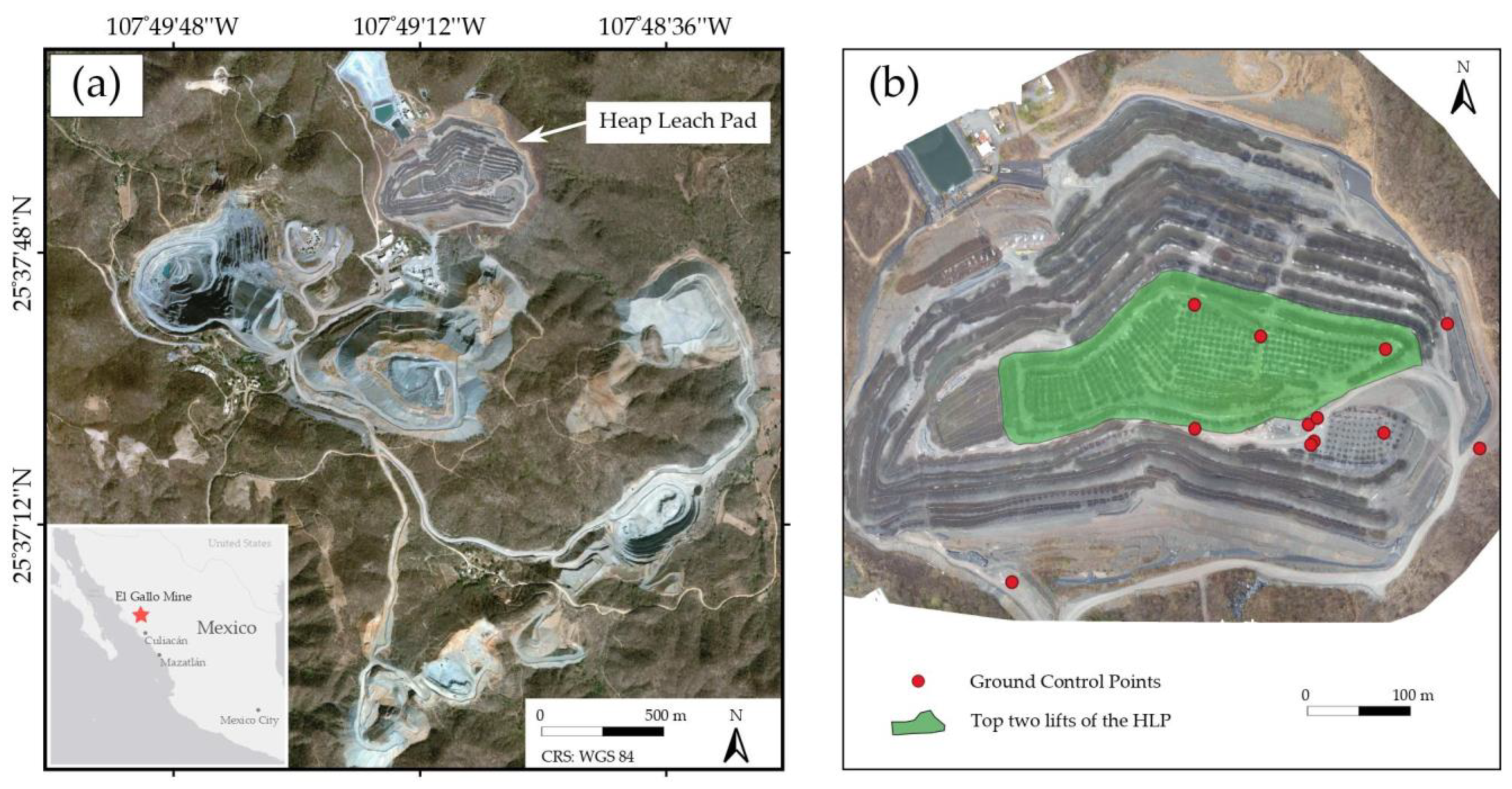
Figure 1. (a) Locations of the El Gallo mine and the studied heap leach pad (HLP); (b) An illustration of the top two lifts of the HLP and the ground control point locations.
Remotesensing 13 01420 g001
Figure 2. (a) An illustration of the heap leach pad’s irrigation system and the unmanned aerial vehicle (UAV) with a dual gimbal setup; (b) The visible-light camera and thermal infrared sensor employed in this study.
Remotesensing 13 01420 g002
Figure 3. Examples of the generated orthomosaics and temperature maps using the collected aerial images. (a,b) are generated based on March 6, Morning datasets; (c,d) are the generated orthomosaic and temperature map, respectively, for the top two lifts of the heap leach pad based on March 8, Afternoon datasets.
Remotesensing 13 01420 g003
Figure 4. (a) Inner structure of the bottleneck residual block used by the ResNet50 architecture; (b) and (c) are the inner structures of the inverted residual blocks in the modified MobileNetV2 architecture with a stride of one and two, respectively. BN stands for batch normalization;Dwise denotes depth-wise convolution; Linear denotes linear activation function.
Remotesensing 13 01420 g004
Figure 5. A schematic illustration of the moisture map generation pipeline of the classification (a) and segmentation (b) approaches.
Remotesensing 13 01420 g005
Figure 6. Classification accuracy of the three employed architectures on the validation set. Each box plot represents the distribution of accuracy for the 30 trained models with the same architecture.
Remotesensing 13 01420 g006
Figure 7. Mean IoU and pixel accuracy of the trained U-Net models on the validation set. Four models failed to converge; thus, each box plot represents the metric values of the 26 converged models.
Remotesensing 13 01420 g007
Figure 8. A comparison of the generated moisture maps for the whole heap leach pad based on the March 8, Afternoon orthomosaic using the classification approach. (ac) are moisture maps generated using the modified AlexNet, ResNet50, and modified MobileNetV2 classifiers, respectively. (d) is the reference moisture map generated by following the same procedure used to prepare the training, validation and testing data for the classification models.
Remotesensing 13 01420 g008
Figure 9. An example of the generated moisture maps using the segmentation approach. (a,c) are the generated moisture maps using the modified U-Net model. (a) is based on the March 8, Afternoon orthomosaic; (c) is based on the March 6, Morning orthomosaic. (b,d) are the corresponding reference moisture maps for (a,c), respectively.
Remotesensing 13 01420 g009
Figure 10. Comparison between the classification- and segmentation-based moisture maps, created using the modified MobileNetV2 and modified U-Net models, respectively. (a) Generated moisture maps for the whole HLP using the classification (left) and segmentation (right) models. (b) Generated moisture maps for the top two lifts of HLP using the classification (left) and segmentation (right) models. (c) Generated moisture maps based on image patches from the segmentation dataset (one from each training, validation, and test set). The upper rows are the input to the models, and the bottom rows are the model outputs. Each input image patch had a size of 64 × 64 pixels.
Remotesensing 13 01420 g010
Table 1. Details of the flight missions for each data collection campaign.
Flight ParametersFlight Mission 1Flight Mission 2
Region of interestTop two lifts of the HLPWhole HLP
Flight altitude90 m120 m
Flight duration7 min24 min
Area surveyed4 ha22 ha
Ground sampling distance (RGB)2.3 cm/pixel3.0 cm/pixel
Ground sampling distance (thermal)12 cm/pixel15 cm/pixel
Table 2. The number of aerial images collected during the field experiment.
6 March 20197 March 20198 March 2019
MorningAfternoonMorningAfternoonMorningAfternoon
Whole HLP *T: 620T: 618T: 618T: 621T: 618T: 619
C: 273C: 281C: 270C: 289C: 290C: 275
Top two lifts *T: 178T: 170T: 174T: 169T: 170T: 173
C: 58C: 74C: 74C: 81C: 73C: 76
* T: number of thermal images; C: number of color (RGB) images.
Table 3. Statistics of the classification dataset.
Moisture
Classes
Whole Dataset (125,252 Images)Training Set (84,528 Images)Validation Set (20,008 Images)Test Set (20,716 Images)
“Dry”37,25124,85156966704
“Moderate”68,11544,25010,67913,186
“Wet”19,88615,4273633826
Table 4. Statistics of the segmentation dataset.
Moisture
Classes
Whole Dataset
(128.3 M Pixels)
Training Set
(86.6 M Pixels)
Validation Set
(20.5 M Pixels)
Test Set
(21.2 M Pixels)
“Dry”31.3%30.8%30.1%34.1%
“Moderate”51.3%49.4%50.3%60.2%
“Wet”17.4%19.8%19.6%5.7%
Table 5. Architecture of the modified AlexNet implemented in this study.
Layer NameLayer Output Dimension
(Height × Width × Channel)
OperationStride
Input32 × 32 × 4--
Conv130 × 30 × 96Conv 3 × 3, 961
Conv228 × 28 × 256Conv 3 × 3, 2561
MaxPool114 × 14 ×256Max pool 2 × 22
Conv314 × 14 × 384Conv 3 × 3, 384, padding 11
Conv414 × 14 × 384Conv 3 × 3, 384, padding 11
Conv514 × 14 × 256Conv 3 × 3, 256, padding 11
MaxPool27 × 7 × 256Max pool 2 × 22
FC11 × 1 × 1024Flatten, 1024-way FC-
FC21 × 1 × 10241024-way FC-
FC3 (Output)1 × 1 × 3Three-way FC, softmax-
Table 6. Architecture of ResNet50.
Layer/Block NameLayer/Block
Output Dimension
OperationStride
Input32 × 32 × 4--
Conv116 × 16 × 64Conv 7 × 7, 642
MaxPool18 × 8 × 64Max pool 3 × 32
Block1_x8 × 8 × 256 [ Conv   1 × 1 ,   64 Conv   3 × 3 ,   64 Conv   1 × 1 ,   256 ] × 3 1
Block2_x4 × 4 × 512 [ Conv   1 × 1 ,   128 Conv   3 × 3 ,   128 Conv   1 × 1 ,   512 ] × 4 1
Block3_x2 × 2 × 1024 [ Conv   1 × 1 ,   256 Conv   3 × 3 ,   256 Conv   1 × 1 ,   1024 ] × 6 1
Block4_x1 × 1 × 2048 [ Conv   1 × 1 ,   512 Conv   3 × 3 ,   512 Conv   1 × 1 ,   2048 ] × 3 1
FC (Output)1 × 1 × 3Global avg. pool, three-way FC, softmax-
Table 7. Architecture of the modified MobileNetV2 implemented in this study.
Layer/Block NameLayer/Block
Output Dimension
OperationStride for 3 × 3 Convolution
Input32 × 32 × 4--
Conv116 × 16 × 32Conv 3 × 3, 322
Block016 × 16 × 16 [ Conv   1 × 1 ,   32 Dwise   Conv   3 × 3 ,   32 Conv   1 × 1 ,   16 ] 1
Block18 × 8 × 24 [ Conv   1 × 1 ,   96 Dwise   Conv   3 × 3 ,   96 Conv   1 × 1 ,   24 ] 2
Block28 × 8 × 24 [ Conv   1 × 1 ,   144 Dwise   Conv   3 × 3 ,   144 Conv   1 × 1 ,   24 ] 1
Block34 × 4 × 32 [ Conv   1 × 1 ,   144 Dwise   Conv   3 × 3 ,   144 Conv   1 × 1 ,   32 ] 2
Block44 × 4 × 32 [ Conv   1 × 1 ,   144 Dwise   Conv   3 × 3 ,   144 Conv   1 × 1 ,   32 ] 1
Block54 × 4 × 32 [ Conv   1 × 1 ,   192 Dwise   Conv   3 × 3 ,   192 Conv   1 × 1 ,   32 ] 1
Conv24 × 4 × 1280Conv 1 × 1, 12801
FC (Output)1 × 1 × 3Global avg. pool, three-way FC, softmax-
Table 8. Architecture of the modified U-Net implemented in this study. All convolutional (Conv), up-convolutional (Up-Conv), and Conv 1 × 1 layers used a stride of 1. The Conv 3 × 3 layers used a padding of 1.
Block/Layer Name Operation Output Dimension
(Height × Width × Channel)
Input-64 × 64 × 4
Encoder1 [ Conv   3 × 3 ,   64 Conv   3 × 3 ,   64 ] 64 × 64 × 64
MaxPool1Max pool 2 × 2, stride 232 × 32 × 64
Encoder2 [ Conv   3 × 3 ,   128 Conv   3 × 3 ,   128 ] 32 × 32 × 128
MaxPool2Max pool 2 × 2, stride 216 × 16 × 128
Encoder3 [ Conv   3 × 3 ,   256 Conv   3 × 3 ,   256 ] 16 × 16 × 256
MaxPool3Max pool 2 × 2, stride 28 × 8 × 256
Encoder4 [ Conv   3 × 3 ,   512 Conv   3 × 3 ,   512 ] 8 × 8 × 512
UpConv1Up-Conv 3 × 3, 25616 × 16 × 256
Concatenation1Concatenate output of Encoder316 × 16 × 512
Decoder1 [ Conv   3 × 3 ,   256 Conv   3 × 3 ,   256 ] 16 × 16 × 256
UpConv2Up-Conv 3 × 3, 12832 × 32 × 128
Concatenation2Concatenate output of Encoder232 × 32 × 256
Decoder2 [ Conv   3 × 3 ,   128 Conv   3 × 3 ,   128 ] 32 × 32 × 128
UpConv3Up-Conv 3 × 3, 6464 × 64 × 64
Concatenation3Concatenate output of Encoder164 × 64 × 128
Decoder3 [ Conv   3 × 3 ,   64 Conv   3 × 3 ,   64 ] 64 × 64 × 64
Conv1Conv 1 × 1, 3, softmax64 × 64 × 3
OutputPixel-wise Argmax64 × 64 × 1
Table 9. Statistical test results of the two-sample Kolmogorov–Smirnov (KS) test and Wilcoxon rank-sum (WRS) test for the there distributions shown in Figure 6.
Tested ModelsKS Test ResultWRS Test Result
Statistically Similar
(5% Significance)
p-ValuesStatistically Similar
(5% Significance)
p-Values
AlexNet—ResNet50No0.0025No0.0493
AlexNet—MobileNetV2No0.0025No0.0006
ResNet50—MobileNetV2Yes0.5941Yes0.7789
Table 10. Confusion matrices and overall accuracies of the three models on the test set (all numbers in %).
ModelPredicted ClassTrue Class Label
DryModerateWet
Modified AlexNet
Overall Accuracy: 98.4
Dry98.80.50
Moderate1.299.115.4
Wet00.484.6
ResNet50
Overall Accuracy: 99.2
Dry99.30.20
Moderate0.799.33.4
Wet00.596.6
Modified MobileNetV2
Overall Accuracy: 99.1
Dry99.50.40
Moderate0.599.02.9
Wet00.697.1
Table 11. Confusion matrix, per-class F1 score, intersection over union (IoU), mean IoU (MIoU), and pixel accuracy (PA) of the modified U-Net model on the test set (all numbers in %).
ModelPredicted LabelTrue Label
DryModerateWet
Modified U-Net
PA: 99.7
MIoU: 98.1
Dry1000.10.0
Moderate0.099.94.6
Wet0.00.095.4
F1 score99.999.797.4
IoU99.999.595.0
Publisher’s Note: MDPI stays neutral with regard to jurisdictional claims in published maps and institutional affiliations.