Estimating Water Vapor Using Signals from Microwave Links below 25 GHz

Abstract

Water vapor is a key element in both the greenhouse effect and the water cycle. However, water vapor has not been well studied due to the limitations of conventional monitoring instruments. Recently, estimating rain rate by the rain-induced attenuation of commercial microwave links (MLs) has been proven to be a feasible method. Similar to rainfall, water vapor also attenuates the energy of MLs. Thus, MLs also have the potential of estimating water vapor. This study proposes a method to estimate water vapor density by using the received signal level (RSL) of MLs at 15, 18, and 23 GHz, which is the first attempt to estimate water vapor by MLs below 20 GHz. This method trains a sensing model with prior RSL data and water vapor density by the support vector machine, and the model can directly estimate the water vapor density from the RSLs without preprocessing. The results show that the measurement resolution of the proposed method is less than 1 g/m³. The correlation coefficients between automatic weather stations and MLs range from 0.72 to 0.81, and the root mean square errors range from 1.57 to 2.31 g/m³. With the large availability of signal measurements from communications operators, this method has the potential of providing refined data on water vapor density, which can contribute to research on the atmospheric boundary layer and numerical weather forecasting.

1. Introduction

Water vapor is a vital greenhouse gas that plays an important role in the water cycle, atmospheric vertical stability, and evolution of a convective storm system [1,2]. Detailed data of near-surface water vapor can help to parameterize the water vapor field in the atmospheric boundary layer and understand the evolution of convective weather [3,4]. However, the accurate estimation of water vapor with a high temporal and spatial resolution still needs to be improved within established methods, including in situ measurements by humidity gauges and satellites or ground-based remote sensing [4,5]. Therefore, developing a technique for estimating near-surface water vapor density with a high temporal-spatial resolution is urgent.

Commercial microwave links (MLs), ranging from 10 GHz to 30 GHz, have been investigated for rainfall estimations in recent years because the signal of ML is attenuated by the rainfall, which can derive the rain rate from the rain-induced attenuation [6,7,8,9,10,11,12,13]. Applications of MLs for estimating rainfall have the following advantages: redundancy, complementarity, timeliness, and low cost [14]. Besides rainfall, the water vapor can also attenuate the signal [15]. Thus, researchers have studied the potential of estimating water vapor density by MLs [16]. David and colleagues first proposed a method for estimating the water vapor density by MLs [17,18]. They estimated the water vapor in central Israel by around 22 GHz MLs based on an attenuation model of the gases [19]. The correlation coefficient of water vapor measurement between the ML and the humidity gauges was 0.82, indicating that MLs have the potential of overcoming the obstacles of the existing methods for monitoring near-surface water vapor. Chwala and colleagues estimated the water vapor density using MLs (22.235 GHz and 34.8 GHz) in Southern Germany [20]. Due to the coherence and the high phase stability of MLs in their study, they derived the water vapor density from the phase delay measurement. The result showed good agreement with the humidity gauges. However, MLs with high phase stability are rare in reality. Additionally, Alpert and Rubin estimated the daily maps of surface moisture from 238 MLs in Israel. They found high correlations (≥0.75) between the MLs’ water vapor field and the weather stations, showing the potential of providing high spatial resolution data of water vapor from MLs [16].

In the previous method of estimating the water vapor density by MLs, the first step of estimating the water vapor density by MLs is extracting the attenuation due to the water vapor from the total attenuation (received signal level, RSL) of the ML. However, compared with the attenuation caused by other factors, such as rainfall and free-space loss, the attenuation by the water vapor is too small to extract accurately, which could increase estimation error. To overcome this problem, we analyze the relationship between the RSL measured by MLs at 15, 18, and 23 GHz and the water vapor density measured by the automatic weather stations (AWS). AWSs are a widely used and accurate point-measurement instrument, which can estimate the near-surface meteorological elements in weather stations [5]. To assure the quality of data measured by AWS, it has been calibrated by the manufacturer and installed according to the guidelines presented by the World Meteorology Organization (WMO) [5]. Then we propose a model between the water vapor density and the RSL of MLs based on available data, directly, by using the support vector machine (SVM). The model can estimate the water vapor density at the station level using the RSL of MLs, which avoids the extraction of the attenuation due to the water vapor from the RSL and reduces the estimation error. Finally, we test the model in an experiment. The water vapor density at the station level has a crucial role in the model initialization in numerical weather prediction, which influences the accuracy of the weather prediction [16]. Besides, it also helps to parameterize the weather model development process [2]. The method proposed in this study can provide refined data on water vapor density and contribute to research on the atmospheric boundary layer.

This study is organized as follows: Section 2 introduces the ML data and details of the proposed method for estimating water vapor density. Section 3 tests the method. Section 4 discusses and concludes the study.

2. Materials and Methods

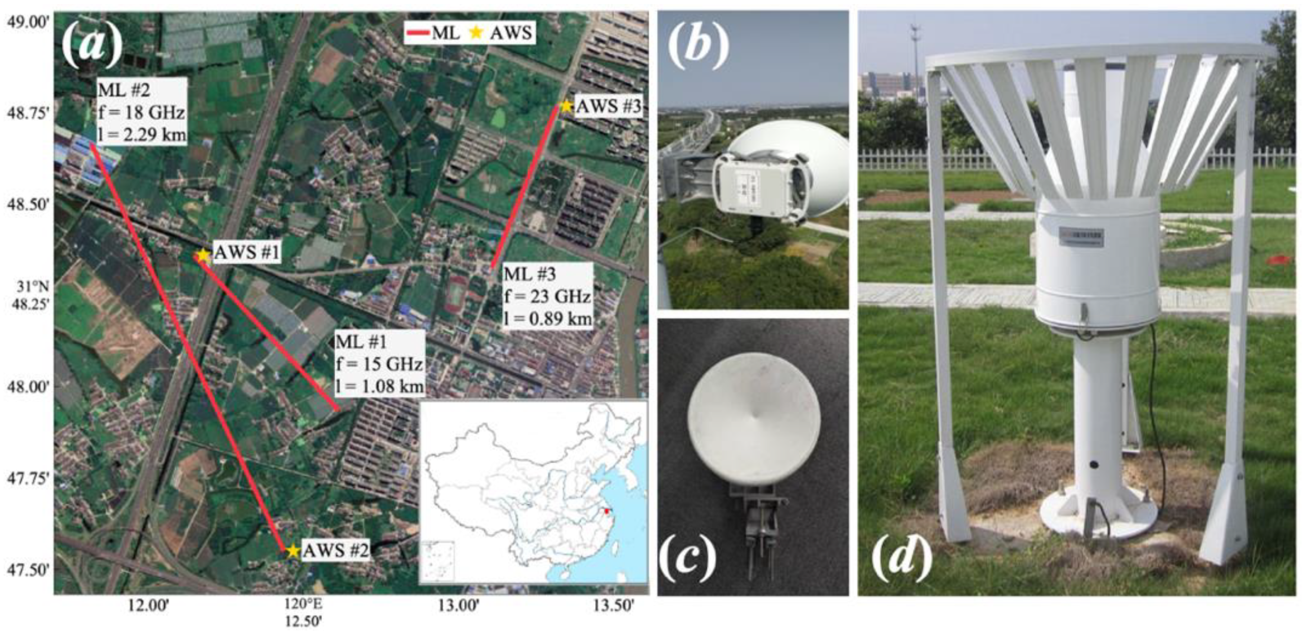
2.1. Data

Three horizontal polarization MLs, at frequencies of 15, 18, and 23 GHz, were applied for this study in Jiangyin, China, from 26 March to 20 April 2019. The MLs consisted of the transmitter and the receiver and were installed on base towers at 30 m, which are operated by China Mobile. The MLs had a constant transmission power and recorded RSLs at 1-minute intervals with a quantization level of 0.1 dB. Records of RSLs were sent to a database server via Global System for Mobile Communications (GSM) without any process from operators. Figure 1a shows the locations, frequencies, and lengths of three MLs, and Figure 1b,c show the transmitter and receiver of the ML. To quantify and validate the results estimated by the MLs, three DZZ-4 Automatic Weather Stations (AWS), from Newsky Corporation, China, were installed near the MLs. The AWS consisted of the water vapor sensor, the rainfall gauge, and other sensors in our experiment. The water vapor sensor was a hygrometer, which could measure the water vapor density with the quantization level of 1 g/m³ and the measurement bias of ± 3% at 5-minute intervals. The rain gauge could measure the rainfall depth with the quantization level of 0.5 mm and the measurement bias of ± 3%. The locations of the AWSs are also shown in Figure 1a. Figure 1d shows a DZZ-4 AWS in the experiment. In this study, both the MLs and the AWSs may miss some measurements. Thus, the dates when the RSLs and the data of the water vapor were measured at the same time were selected for the test. In the study, ML #1 recorded 19 non-rainy days and 1 rainy day, ML #2 recorded 17 non-rainy days and 2 rainy days, and ML #3 recorded 14 non-rainy days and 2 rainy days.

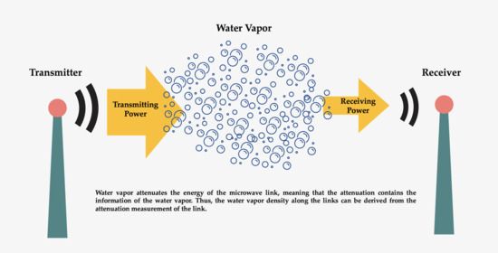
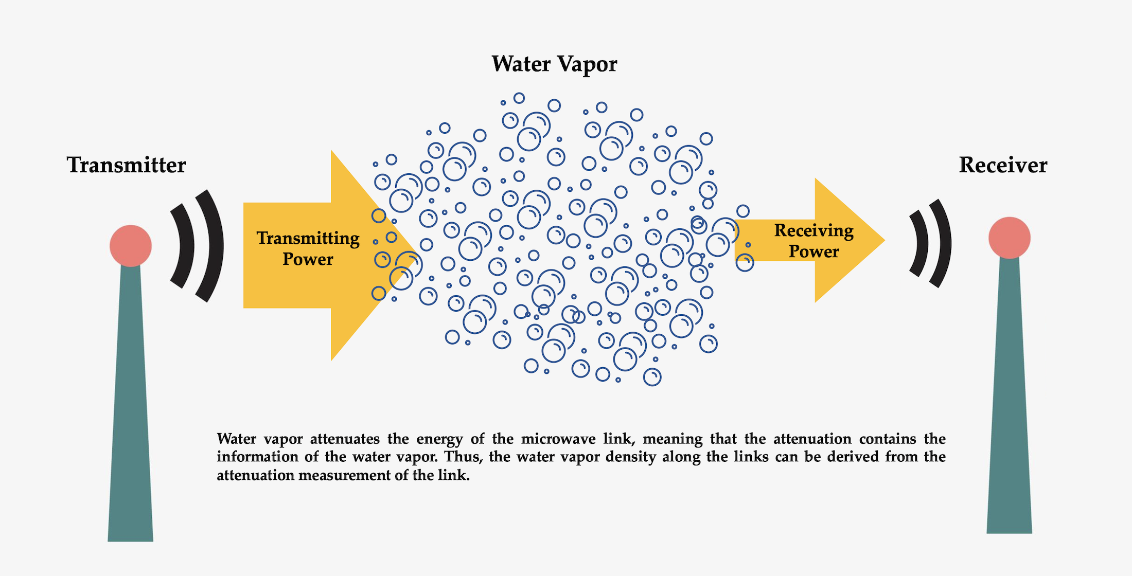
2.2. Analysis of the Potential of Estimating Water Vapor with the ML Attenuation Signal

The water vapor attenuates the energy of the ML in the transmission path with the following equation [18,19]:

$$\{\begin{array}{l}{\gamma }_w=0.1820\times f\cdot N^{″}{}_w(f,P,T,\rho )\\ A_w={\gamma }_w\cdot l\end{array}$$

(1)

where ${\gamma }_w$ and A_w are the water vapor-induced attenuation rate (dB/km) and the water vapor-induced attenuation (dB), respectively, and $N^{″}{}_w(f,P,T,\rho )$ is the imaginary part of the frequency-dependent complex refractivity, which is a function of frequency (f, GHz), atmospheric pressure (P, hPa), air temperature (T, °C), and water vapor density (ρ, g/m³), l is the length of the ML (km). The detailed calculation of $N^{″}{}_w(f,P,T,\rho )$ is given in [19]. Note that in meteorological practice, it is customary to use relative humidity (%) to represent the level of water vapor. The relationship between the water vapor density and the relative humidity is as follows:

$$\rho =1324.45+\frac{RH}{100\%}\times \frac{\exp \left(17.67\cdot T\right)}{T+273.15}$$

(2)

where RH represents the relative humidity. Figure 2 shows ${\gamma }_w$ with different frequencies and values of ρ, which is calculated by (1). The water vapor-induced attenuation peak was located between 22 and 23.5 GHz below 50 GHz, and ${\gamma }_w$ increased as ρ increased. Meanwhile, the measurement resolution of ρ at 1 km and a 23 GHz ML with 0.1 dB quantization is given in the top left subfigure of Figure 2. It shows that both the measurement sensitivity and the measurement resolution were approximately 4 g/m³. It meant that the minimum value of ρ that could be measured was 4 g/m³, and the minimum variation of ρ that could be measured was also 4 g/m³, which is one of the highest sensitivities and resolutions below 50 GHz. Note that the peak frequency of the water vapor absorption was 22.235 GHz [20].

In theory, ρ along the ML could be retrieved on the condition that A_w was extracted from the RSL measured by a ML-based on Equation (1) [17,18]. The first step was to determine the baseline, which was defined as the attenuation other than the water vapor [18]. Figure 3a shows the RSL of ML #3 and the ρ measured by AWS #3. Note that the RSL was calculated by the 5-minute average of the attenuation because the sample time of the AWS was 5 minutes. A positive correlation between the RSL and ρ is displayed in Figure 3a, and the correlation coefficient (CC) was 0.76, which indicated that the ML could sense the variation of the water vapor. We measured the water vapor density by AWSs in this study. Thus, A_w of the ML, in theory, could be calculated by Equation (1). Then, the baseline, in theory, could be also obtained by the following equation:

baseline = A_m − A_w

(3)

Figure 3b shows a comparison between the RSL and A_w in theory, and Figure 3c shows the RSL and the baseline in theory. Figure 3b shows that A_w was much smaller than the RSL, and Figure 3c shows the baseline rapidly and continuously changed, which meant that A_w was easily hidden in the RSL with inaccurate baseline determinations and measurement noises in reality. Therefore, the method of extracting A_w from the ML may not be suitable at such low frequencies (lower than 50 GHz) in order to estimate ρ [18].

Figure 4 shows the time series comparison between the RSL and ρ of MLs #1–3 on non-rainy days. Although it was difficult to extract accurate A_w from the MLs, the RSLs of the three MLs sensed the variations of ρ with the positive correlation. The CC between the RSL and ρ for each day during the experiment is also given in Figure 4. Most values of CC were higher than 0.6, and the highest values were over 0.9, which revealed that the RSL correlated to ρ in a positive manner. Even for a 15-GHz ML whose values of A_w were too small to estimate ρ by the method proposed in [18], the RSL could still sense ρ well. Therefore, we could derive ρ by establishing the model between the RSL and ρ.

2.3. Estimating the Water Vapor Density by MLs Based on SVM

In the study, the SVM is adopted for establishing the model between the RSL and ρ. The SVM is an extensively employed machine learning method with a set of linear indicator functions for classification and regression analysis [21]. The SVM maps the input data into a high-dimensional feature space where a hyperplane is constructed. Compared with other machine learning methods, the SVM is more suitable for data with small sample size, for example, estimating ρ in this study.

We set $RS{L}_{T,i}$ and ${\rho }_{T,i}$ as the training set, where $RS{L}_{T,i}$ is the RSL measurement, ${\rho }_{T,i}$ is the true water vapor density, i represents the time series from 1 to N, and N represents the length of the training set. First, the optimal solution of the convex quadratic programming problem was constructed and solved:

$$\begin{array}{l}\underset{\alpha }{\min }\frac{1}{2}{\displaystyle \sum _{i=1}^N{\displaystyle \sum _{j=1}^N{\alpha }_i\cdot {\alpha }_j\cdot {\rho }_{T,i}\cdot {\rho }_{T,j}\cdot K(RS{L}_{T,i}\cdot RS{L}_{T,j})}-{\displaystyle \sum _{i=1}^N{\alpha }_i}}\\ s.t.\{\begin{array}{l}{\displaystyle \sum _{i=1}^N{\alpha }_i\cdot {\rho }_{T,i}}=0\\ 0\le {\alpha }_i\le C,i=1,2,3,\cdots ,N\end{array}\end{array}$$

(4)

where K(·) is the radial basis kernel function, and C is a positive penalty parameter. Thus, the optimal solution, α^*, was solved by Equation (4). The weight of the regression function (ω^*) could be calculated as follows:

$${\omega }^{*}={\displaystyle \sum _{i=1}^N{\alpha }_i^{*}\cdot {\rho }_{T,i}\cdot RS{L}_{T,i}}$$

(5)

Next, the constant threshold, b, could be calculated:

$$b^{*}={\rho }_{T,j}-{\displaystyle \sum _{i=1}^N{\alpha }_i^{*}\cdot {\rho }_{T,i}\cdot K(RS{L}_{T,i}\cdot RS{L}_{T,j})}$$

(6)

Finally, the regression function was obtained:

$$f(RS{L}_i)={\omega }^{\mathrm{T}}\cdot K(RS{L}_T,RS{L}_i)+b$$

(7)

where $f(RS{L}_i)$ is the water vapor density, and RSL_i is the real-time attenuation measurement. Equation (7) is the model between the RSL and ρ, and we could estimate ρ by inputting the measurements of the RSL into the model.

3. Results

3.1. Training and Test Dataset for the SVM Model

In this study, daily data was used as the single test set for estimating ρ. Thus, the dates before the test date were adopted as the training set to train the model. Note that the data of the first day of the three MLs weres not selected as the test set because there was no training set for it. The measurements of the RSL of the test sets were input into the model, and then the estimated values of the water vapor density ($\widehat{\rho }$) were output. Note that $\widehat{\rho }$ from the ML is a path-average value, while the value measured by the AWS is a point value, which means that these two results cannot be fully consistent.

3.2. Estimating the Water Vapor Density on Non-Rainy Days

Figure 5a,c,e show the comparisons between the true water vapor density (ρ) by the AWSs and $\widehat{\rho }$ by the MLs. The results showed a positive correlation between ρ and $\widehat{\rho }$, which indicated that the MLs have the potential of estimating the water vapor density. Meanwhile, a quantitative calculation of CC and the root mean square error (RMSE) for $\widehat{\rho }$ is also given in the figure. The CC values were higher than 0.7, which further indicated the positive relationship between ρ and $\widehat{\rho }$. Moreover, the RMSE values ranged from 1.57 to 2.31 g/m³. Although the frequency of ML #2 was lower than the frequency of ML #3, ML #2’s result was better than ML #3’s. This was because the length of ML #2 was much longer than that of ML #1, leading to a more serious influence on ML #2 by the water vapor.

In addition, Figure 5b,d,f show the scatter plots between the RSL and $\widehat{\rho }$. Additionally, linear relations between them were also given by the linear regression. Taking Figure 5f as an example, the slope of the regression line was 7.94, and the quantization level of the RSL was 0.1 dB, which meant that the measurement resolution of the water vapor density by ML #3 was approximately 0.8 g/m³ in theory, which was much higher than that of the method (approximately 4 g/m³ at 23 GHz) mentioned in [18] at the same frequency. However, the analysis was not suitable for ML #1 because the accuracy was much lower than the other MLs. Since a marked daily cycle is shown in Figure 5a,c,e, we compared the water vapor anomaly of the same time between ρ and $\widehat{\rho }$ in Figure 6. It shows that the deviation of $\widehat{\rho }$ from the average water vapor density was similar to ρ for ML #2 and ML #3, which further proved that MLs can estimate the variation of the water vapor. The anomaly of ML #1 between ρ and $\widehat{\rho }$ had biases in some days because the frequency was low, leading to the weak water vapor effect of the attenuation.

Figure 7 gives the results of retrieving the water vapor density by THE ML based on the general methods in previous works [16,17,18]. In these works, they estimated the water vapor density by Equation (1), which is proposed by International Telecommunication Union (ITU) [19]. Figure 7a shows that ML #1 WAs unable to estimate the water vapor density by the ITU model because the water vapor-induced attenuation was too small to be measured by MLs at 15 GHz. Figure 7b shows that ML #2 could estimate the water vapor density by the ITU model. However, compared with Figure 5b, values of the CC and RMSE were lower, meaning that the SVM model proposed in this study had a higher accuracy of the estimation. Besides, the measurement resolution of the ITU model was around 6 g/m³, while that of the SVM model was around 1 g/m³. As for ML #3, the values of the CC and RMSE by the ITU model were higher than the values by the SVM model, because the frequency of ML #3 was located in the water vapor absorption band [19], leading to the obvious water vapor induced attenuation. But the measurement resolution of the SVM model was better than the ITU model. As can be seen from Figure 7, the SVM model had advantages on the estimation accuracy and the measurement resolution other than at the water vapor absorption band. At the water vapor absorption band, the estimation accuracy of the ITU model was slightly better, while the SVM model had a better measurement resolution. Additionally, the SVM model could be used at more frequencies, even the water vapor-induced attenuation was weak, which was more practical because the frequencies at the water vapor absorption band were less in reality.

3.3. Estimating the Water Vapor Density on Rainy Days

It is well known that rainfall also attenuates the energy of MLs, and rain-induced attenuation is much higher than A_w [6,15,19,22]. Thus, A_w can be easily submerged by rain-induced attenuation. To address this issue, a test was conducted for estimating the water vapor density on rainy days. The variation of the RSL on rainy days could be different from that on non-rainy days, which means that the model needs to be trained by the data by rainy days. MLs #2 and 3 were chosen for the test because they measured two-day data. Figure 8a and b show the results, and Figure 8c shows the time-series for the rain rate on 9 April 2019. It rained for approximately 2 h from 12:40 to 14:45 on 9 April 2019. The CC values for the two MLs between ρ and $\widehat{\rho }$ were 0.89 and 0.64, respectively, which meant that the ML could still sense the variation in water vapor on rainy days. Before the rain started, the RMSE values were 0.52 g/m³ and 0.74 g/m³, respectively. During the rain, the RMSE values changed to 0.93 g/m³ and 2.83 g/m³, respectively, which indicated that the rainfall influenced the estimation accuracy. After the rain, the accuracy of ML #2 returned to the level before the rain, while the accuracy of ML #3 still remained similar to the accuracy during the rain. The most possible reason was that the wet surfaces of the antennas of the ML during and after the rain lead to the wet antenna attenuation [23,24]. Wet antenna attenuation is related to the frequency of the ML, surface material, and the amount of water accumulated on the surfaces, which causes rapid and deep fluctuations in the attenuation of the ML [24,25,26,27]. Thus, it leads to the phenomenon in the experiment. Further work needs to be done in the future due to the lack of data for rainy days. We will carry out more experiments to investigate the feasibility of estimating the water vapor by ML in the rain. For this purpose, the rain-induced attenuation and the wet antenna attenuation should be excluded from the RSL of the ML. Rain-induced attenuation may be calculated because the ML could estimate the rain in previous studies [6,7,8,9,10,11]. The wet antenna attenuation should also be modeled by some methods such as machine learning [27]. Then we will estimate the water vapor based on the correction RSL by using the SVM method. However, it may affect the estimation accuracy negatively during the rain, because the rain-induced attenuation is much larger. Therefore, it is essential to obtain the rain-induced attenuation, precisely.

4. Discussion and Conclusions

This study describes a preliminary analysis of the relation between the RSL measured by MLs at 15, 18, and 23 GHz and the water vapor density. We propose a method for estimating the water vapor density using the RSL of MLs. Different from the previous method using MLs [17,18], this method trains a model between the RSL and the water vapor density by the SVM, and then the model can estimate the water vapor density by inputting the RSL. However, this method requires the prior data of the RSL and the corresponding water vapor density to train the model. Despite this limitation, the method can avoid extracting the true water vapor-induced attenuation, which can reduce the error.

More importantly, the measurement resolution of the water vapor density (approximately 0.8 g/m³) is much higher than the resolution (approximately 4 g/m³ at 23 GHz) in [18]. A positive correlation and RMSEs between ρ and $\widehat{\rho }$ in Figure 5 indicate that the ML has the potential of estimating water vapor density. Additionally, the results on rainy days show that the RMSE values will increase when rain starts, which indicates that rainfall can influence the accuracy. However, because of the lack of data on rainy days, more measurements and analyses for estimating water vapor by MLs will be conducted in the future.

References

1. Weckwerth, T.M.; Murphey, H.V.; Flamant, C.; Goldstein, J.; Pettet, C.R. An observational study of convection initiation on 12 June 2002 during IHOP_2002. Mon. Weather Rev. 2008, 136, 2283–2304. [Google Scholar] [CrossRef] [Green Version]
2. Muller, C.L.; Chapman, L.; Johnston, S.; Kidd, C.; Illingworth, S.; Foody, G.; Overeem, A.; Leigh, R.R. Crowdsourcing for climate and atmospheric sciences: Current status and future potential. Int. J. Climatol. 2015, 35, 3185–3203. [Google Scholar] [CrossRef] [Green Version]
3. Weckwerth, T.M. The effect of small-scale moisture variability on thunderstorm initiation. Mon. Weather Rev. 2000, 128, 4017–4030. [Google Scholar] [CrossRef]
4. Sherwood, S.C.; Roca, R.; Weckwerth, T.M.; Andronova, N.G. Tropospheric water vapor, convection, and climate. Rev. Geophys. 2010, 48. [Google Scholar] [CrossRef] [Green Version]
5. World Meteorology Organization. Guide to Meteorological Instruments and Methods of Observation, 7th ed.; World Meteorology Organization: Geneva, Switzerland, 2008. [Google Scholar]
6. Messer, H.; Zinevich, A.; Alpert, P. Environmental Monitoring by Wireless Communication Networks. Science 2006, 312, 713. [Google Scholar] [CrossRef] [PubMed] [Green Version]
7. Berne, A.; Uijlenhoet, R. Path-averaged rainfall estimation using microwave links: Uncertainty due to spatial rainfall variability. Geophys. Res. Lett. 2007, 34. [Google Scholar] [CrossRef] [Green Version]
8. Leijnse, H.; Uijlenhoet, R.; Stricker, J.N.M. Rainfall measurement using radio links from cellular communication networks. Water Resour. Res. 2007, 43, 455–456. [Google Scholar] [CrossRef]
9. David, N.; Alpert, P.; Messer, H. The potential of cellular network infrastructures for sudden rainfall monitoring in dry climate regions. Atmos. Res. 2013, 131, 13–21. [Google Scholar] [CrossRef]
10. Doumounia, A.; Gosset, M.; Cazenave, F.; Kacou, M.; Zougmore, F. Rainfall Monitoring based on Microwave links from cellular telecommunication Networks: First Results from a West African Test Bed. Geophys. Res. Lett. 2014, 41, 6016–6022. [Google Scholar] [CrossRef]
11. Overeem, A.; Leijnse, H.; Uijlenhoet, R. Two and a half years of country-wide rainfall maps using radio links from commercial cellular telecommunication networks. Water Resour. Res. 2016, 52, 8039–8065. [Google Scholar] [CrossRef] [Green Version]
12. Smiatek, G.; Keis, F.; Chwala, C.; Fersch, B.; Kunstmann, H. Potential of commercial microwave link network derived rainfall for river runoff simulations. Environ. Res. Lett. 2017, 12, 034026. [Google Scholar] [CrossRef] [Green Version]
13. Uijlenhoet, R.; Overeem, A.; Leijnse, H. Opportunistic remote sensing of rainfall using microwave links from cellular communication networks. WIREs Water 2018, 5. [Google Scholar] [CrossRef] [Green Version]
14. Cherkassky, D.; Ostrometzky, J.; Messer, H.; Sensing, R. Precipitation Classification Using Measurements from Commercial Microwave Links. IEEE Trans. Geosci. Remote Sens. 2014, 52, 2350–2356. [Google Scholar] [CrossRef]
15. ITU-R. Specific Attenuation Model for Rain for Use in Prediction Methods; International Telecommunication Union: Geneva, Switzerland, 2005. [Google Scholar]
16. Alpert, P.; Rubin, Y. First Daily Mapping of Surface Moisture from Cellular Network Data and Comparison with Both Observations/ECMWF Product. Geophys. Res. Lett. 2018, 45, 8619–8628. [Google Scholar] [CrossRef]
17. David, N.; Alpert, P.; Messer, H. Technical Note: Novel method for water vapour monitoring using wireless communication networks measurements. Atmos. Chem. Phys. 2009, 9, 2413–2418. [Google Scholar] [CrossRef] [Green Version]
18. David, N.; Sendik, O.; Rubin, Y.; Messer, H.; Gao, H.O.; Rostkier-Edelstein, D.; Alpert, P. Analyzing the ability to reconstruct the moisture field using commercial microwave network data. Atmos. Res. 2019, 219, 213–222. [Google Scholar] [CrossRef]
19. ITU-R. Attenuation by Atmospheric Gases. 2016. Available online: https://www.itu.int/dms_pubrec/itu-r/rec/p/R-REC-P.676-11-201609-I!!PDF-E.pdf (accessed on 4 April 2021).
20. Chwala, C.; Kunstmann, H.; Hipp, S.; Siart, U. A monostatic microwave transmission experiment for line integrated precipitation and humidity remote sensing. Atmos. Res. 2014, 144, 57–72. [Google Scholar] [CrossRef] [Green Version]
21. Vapnik, V. The Nature of Statistical Learning Theory; Springer Science & Business Media: Berlin, Germany, 2013. [Google Scholar]
22. Minda, H.; Nakamura, K. High Temporal Resolution Path-Average Rain Gauge with 50GHz Band Microwave. J. Atmos. Ocean. Technol. 2005, 22, 165–179. [Google Scholar] [CrossRef]
23. Kharadly, M.M.Z.; Ross, R. Effect of wet antenna attenuation on propagation data statistics. IEEE Trans. Antennas Propag. 2001, 49, 1183–1191. [Google Scholar] [CrossRef]
24. Leijnse, H.; Uijlenhoet, R.; Stricker, J.N.M. Microwave link rainfall estimation: Effects of link length and frequency, temporal sampling, power resolution, and wet antenna attenuation. Adv. Water Resour. 2008, 31, 1481–1493. [Google Scholar] [CrossRef]
25. Schleiss, M.; Rieckermann, J.; Berne, A. Quantification and Modeling of Wet-Antenna Attenuation for Commercial Microwave Links. IEEE Geosci. Remote Sens. Lett. 2013, 10, 1195–1199. [Google Scholar] [CrossRef]
26. Fencl, M.; Valtr, P.; Kvicera, M.; Bares, V. Quantifying Wet Antenna Attenuation in 38-GHz Commercial Microwave Links of Cellular Backhaul. IEEE Geosci. Remote Sens. Lett. 2019, 16, 514–518. [Google Scholar] [CrossRef]
27. Pu, K.; Liu, X.; He, H. Wet Antenna Attenuation Model of E-band Microwave Links Based on the LSTM Algorithm. IEEE Antennas Wirel. Propag. Lett. 2021, 19, 1586–1590. [Google Scholar] [CrossRef]
Figure 1. Details of the microwave links (MLs) and automatic weather stations (AWSs). The red point of the bottom right subfigure shows the location of Jiangyin in China in (a). (b,c) show the transmitter and receiver of the ML. (d) shows the DZZ-4 AWS.
Remotesensing 13 01409 g001
Figure 2. Water vapor induced attenuation rates with different frequencies and water vapor density (temperature = 25 °C, pressure = 1013.25 hPa). The red transparent part represents the water vapor absorption band.
Remotesensing 13 01409 g002
Figure 3. Received signal level (RSL) for ML #3 on non-rainy days (15 days) vs. (a) ρ measured by AWS #3, (b) Aw, and (c) the baseline in theory.
Remotesensing 13 01409 g003
Figure 4. Time-series comparison between the RSL and ρ for the MLs (a,c,e) and the correlation coefficient (CC) between the RSL and ρ of each non-rainy day for the MLs (b,d,f). Data for ρ in a, c, and e are measured by AWS #1, 2, and 3, respectively.
Remotesensing 13 01409 g004
Figure 5. Results for ρ ^ on non-rainy days (a,c,e) and scatter plots between the RSL and ρ ^ with the linear regression lines (b,d,f).
Remotesensing 13 01409 g005
Figure 6. Time-series of the water vapor anomaly between ρ and ρ ^ on non-rainy days.
Remotesensing 13 01409 g006
Figure 7. Time-series of the result between the water vapor density by MLs based on the International Telecommunication Union (ITU) model and the measurement by the AWS.
Remotesensing 13 01409 g007
Figure 8. Results of ρ ^ on a rainy day (a,b) and the time-series for rain rates on 9 April 2019 (c). The yellow transparent part represents the rainfall period.
Remotesensing 13 01409 g008
Publisher’s Note: MDPI stays neutral with regard to jurisdictional claims in published maps and institutional affiliations.