Abstract
A country can be well-comprehended through its core cities. Similarly, we can learn about a city from its hotspots, as they manifest the concentration of urban infrastructures and human activities. Following this philosophy, this paper studies the intra-urban form and function from a complexity science perspective by exploring the power law distribution of hotspot sizes and related socio-economic attributes. To detect hotspots, we rely on spatial clustering of geospatial big data sets, including street data from OpenStreetMap platform and nighttime light (NTL) data from the visible infrared imaging radiometer suite (VIIRS) imagery. Unlike conventional spatial units, which are imposed by governments or authorities (such as census block), the delineation of hotspots is done in a totally bottom-up manner and, more importantly, can help us examine precisely the scaling pattern of urban morphological and functional aspects. This results in two types of urban hotspots—street-based and NTL-based hotspots—being generated across 20 major cities in China. We find that Zipf’s law of hotspot sizes (both types) holds remarkably well for each city, as do the city-size distributions at the country level, indicating a statistically self-similar structure of geographic space. We further find that the urban scaling law can be effectively detected when using NTL-based hotspots as basic units. Furthermore, the comparison between two types of hotspots enables us to gain in-depth insights of urban planning and urban economic development.
1. Introduction
As a result of urbanization or the continuous influx of people into cities, the number of worldwide urbanites is predicted to be 6.9 billion by 2050, accounting for 68% of the world’s population [1]. The urbanization in China has been unprecedentedly rapid as well in the past few decades [2], reaching 60.6% nationally in 2019 [3]. Consequently, the grasp of city form and function—that is, how cities look and work—has become the key to our sustainable development. Given the circumstances, city-related research has attracted scientists from a variety of subjects and has, inevitably, become cross-disciplinary, including geography, economics, computer science, and physics, etc. To converge these disciplines, scholars have called for a new science of cities in the past few decades, in which they view cities as an organized complexity [4], for studying cities’ fractal shapes, complex structures, and nonlinear dynamics (e.g., [5,6,7,8,9,10,11]).
One major aspect of urban complexity is its underlying scaling properties. The scaling pattern of urban entities can be categorized into two perspectives: The power law distribution of a single quantity, such as city sizes (Zipf’s law [12]), building heights [13], street lengths [14], and leisure venue densities [15], and the power relationship between two quantities, such as populations versus innovations ([16,17]) or gross domestic product (GDP) versus street fractality ([18,19]). This study uses the terms scaling and power law interchangeably. Urban scaling is, to a great extent, a ubiquitous pattern across different measures. Moreover, the theory developed by Bettencourt et al. [16], which is behind the power relationship between urban populations and other socio-economic measures, has been formulated as fundamental laws about cities: Universal scaling law. However, recent studies have shown that the universal scaling law may not work as expected, as the scaling exponent is sensitive to different city boundaries or ineffective urban areas [20,21]. This controversy is likely to be bound with the top-down methods of defining geographic units by governments and authorities, such as administrative city boundaries, census tracts, and some equally partitioned cells, which are essentially for management purposes and hardly consider the scaling pattern of urban morphological and functional entities.
The arrival of geospatial big data has triggered a new paradigm for urban analysis since geospatial big data, such as remote sensing (RS) images and location-based social media data, has the capacity to offer fine-grained, massive-scale geographic information [22]. For instance, nighttime lights (NTL) data, also referred to as RS of human beings and their activities [23], are globally downloadable and can manifest the development of urban and regional areas. OpenStreetMap (OSM), a pioneering volunteered geospatial information platform, provides street data across the globe for probably the first time in human history [24]. Both NTL and OSM data help researchers construct alternative modeling units for spatial analyses at both intercity and intracity levels, and remove the barriers of inter-regional incomparability. The most recent relevant studies are so-called natural cities, referring to the objectively defined cities based on different types of urban elements from the open data, such as building footprints, street nodes, and points of interest (e.g., [25,26,27,28,29]). However, most of these studies take the derived cities as a whole to understand the scaling structure over a region or country, but seldom calibrate a “local” understanding of such spatial configuration at the intracity level.
Thus, the present study attempts to investigate the intra-urban scaling properties through the lens of city hotspots. A city is formed by highly concentrated areas of human settlements or activities within a country extent [30]. Likewise, if we scale down our scope from a country to one of its cities, such concentrations can be regarded as urban hotspots. With the advance of geographic information system (GIS) technologies, urban hotspots can be delineated more precisely on the support of geospatial big data and bottom-up approaches. The study contributes to the current literature in three aspects. Firstly, we followed the ideas of previous city delineation methods to derive two types of urban hotspots across 20 Chinese cities: Street-based and NTL-based hotspots, from respectively the spatial clustering of individual street nodes and NTL image pixels with the cutoff determined by data’s inherent scaling properties (see details in Section 2.2). Secondly, we found that Zipf’s law held remarkably well for both street-based and NTL-based hotspot sizes per city, as do the city-size distributions on the national scale. The scaling exponents derived based on NTL-based hotspots were also consistent with the established regimes, implying that NTL-based hotspots can act as better spatial units for urban analysis. Thirdly, we found that the spatial discrepancy between the street-based and NTL-based hotspots can lead us to deep insights on urban planning and development.
The remainder of this paper is organized as follows. Section 2 introduces the data sets and the designed methods for urban hotspot delineation and related scaling analyses. Section 3 presents the maps of the detected hotspots across the top 20 cities in China, as well as the power law metrics of hotspot sizes and associated socio-economic attributes. Section 4 further discusses the intra-urban scaling properties. Section 5 concludes the study and points to future research directions.
2. Data and Methods
2.1. Data and Data Processing
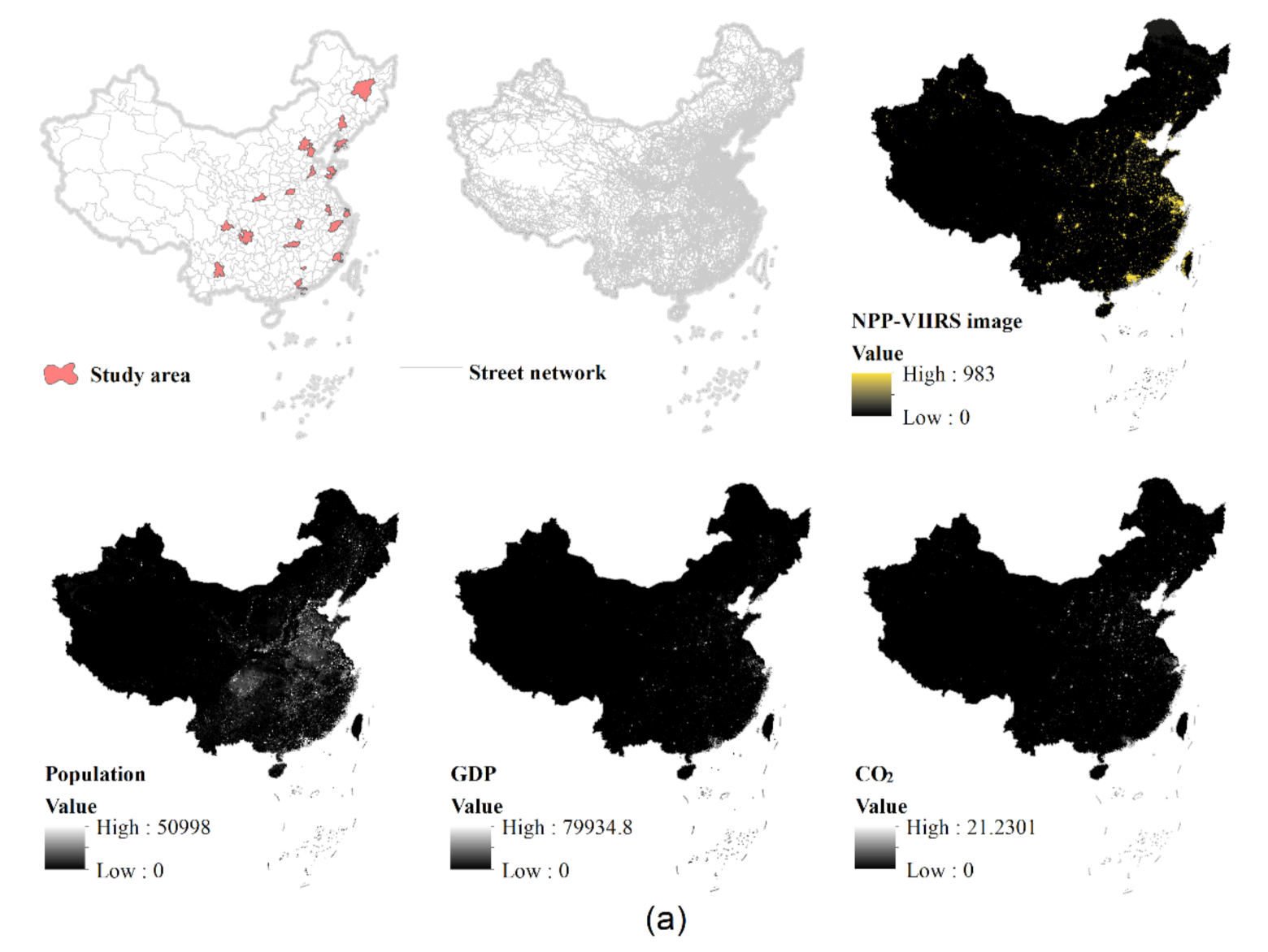
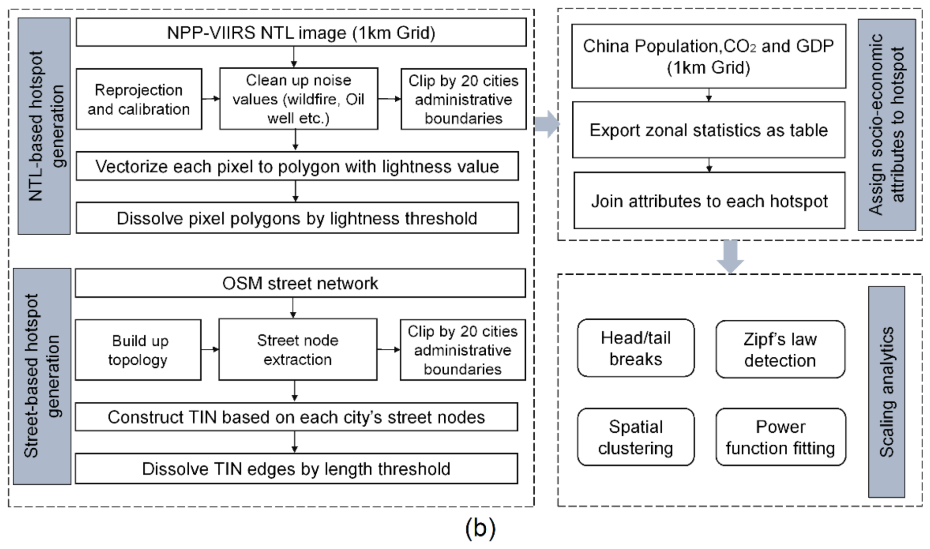
We selected 20 well-developed cities in China as study areas and primarily made use of the following three data sets: (1) VIIRS imagery, (2) OSM street network, and (3) socio-economic grid data (Figure 1a). All data sets are national coverage. The NTL data was obtained from NOAA/NCEI [31]. We chose one monthly image at June 2020, of which the resolution is 15-arc-s (about 500 m at the Equator). We reprojected and cleaned the image to get rid of noises (lit spots) such as burning wildfires and oil drilling, based on the method proposed by Elvidge et al. [32]. The national street network was downloaded from OSM, including 4,419,603 segments from which we extracted 3,172,001 street nodes based on the criterion that a node must intersect with three segments. The socio-economic grid data include the GDP and population from the National Resources and Environment Database of the Chinese Academy of Sciences [33] and environmental grid data include CO2 emissions from the National Earth System Science Data Center [34]. Raster data sets for GDP, population, and CO2 were collected in 2010 and had a 1 km resolution. To perform the analysis, we clipped out both the vector and raster data using each of 20 city administrative boundaries, then conducted zonal statistics of cells with socio-economic attributes for each city, which were further joined with city hotspots (Figure 1b).

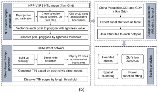
Figure 1.
(Color online) The related datasets (a) and the methodological framework (b) in this study. (Note: The units of raster datasets for population, GDP, CO2 emissions are 1 person/km2, 10,000 CNY/km2, and 10,000 ton/km2, respectively).
2.2. Urban Hotspot Detection
We adopted the spatial clustering method for urban hotspot calculation and delimitation. As there were two types of data sets (street junction nodes and NTL pixels) to be processed, we applied two rules for cluster detection of each data set: Point proximity and lit pixel adjacency. The threshold (distance between points or pixel value) for clustering was determined by the data’s inherent scaling properties uncovered by head/tail breaks and power law detection methods.
2.2.1. Spatial Clustering of Street Nodes and NTL Pixels
Urban hotspots—that is, populated areas in a city—are the basic unit for the analysis in this study. Traditional urban analysis uses pre-defined administrative units provided by local authorities or grids with different resolutions. However, both spatial units cannot represent the merit of “concentration” as they are defined either from a top-down or arbitrary manner. To overcome this issue, we adopted a spatial clustering approach to objectively delimit the boundary of a hotspot from the dense areas of street junctions or lit pixels.
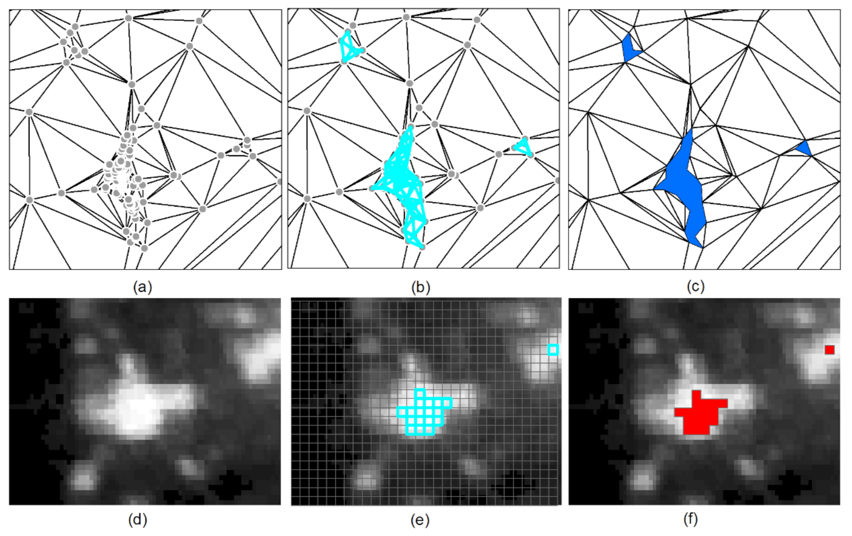
We chose two clustering approaches for each data set. For street junctions, we first computed the triangulated irregular network (TIN) to get junction–junction proximities. As Figure 2a–c shows, the area of urban hotspot can be directly obtained through the conversion of short TIN edges between points. For NTL images, the first step is to vectorize each raster pixel into a polygonal feature with the light value maintained (Figure 2e), then the hotspot can be derived through grouping the adjacent lit pixels (Figure 2f).
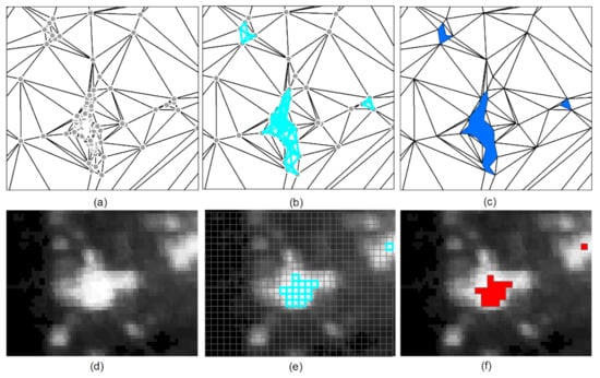
Figure 2.
(Color online) The derivation of urban hotspots using the spatial clustering approach based on respectively street nodes (a–c) and NTL image pixels (d–f).
The above procedures can be simply done using any mainstream GIS or RS image processing software (such as ArcGIS and Erdas). The major difficulty lies in identifying the cutoff value for the classification short/long edges and dim/lit pixels across a set of urban areas. In other words, it lacks an objective criterion to make the linkage between the morphological hotspot (the concentration of urban infrastructure) and a set of proximate street junctions or the functional hotspot (the concentration of human activities) and a group of lit pixels. The same issue occurs when delineating the city boundaries (regardless of administrative boundaries) at the country or cross-country level, whereas prior studies (e.g., [35]) have made use of the universal scaling property for finding the effective cutoff value. In a similar spirit, the next section will introduce how to obtain the optimal cutoff value for the accurate delimitation of urban hotspots.
2.2.2. Scaling Analytics for Identifying the Cutoff for Spatial Clustering
A vast body of literature has investigated city-size distributions in different countries. Most of those studies have used the power law model to characterize the uneven spatial distribution of cities, as well as their sizes, such as Zipf’s law [12]. Zipf’s law states that there is an inverse relationship between the rank and the size of a city. In other words, the largest city is twice as big as the second largest city, etc. Such a statistical distribution would strikingly present the long-tail effect or scaling pattern of far more small cities than large ones. In most cases, the scaling pattern recurs within the power-law distribution and leads to an inherent hierarchy, which can be derived through the head/tail breaks classification scheme. In this study, we change our perspective from a “country-to-city” relationship to “city-to-hotspot” one. In this way, we can borrow the scaling analysis methods (power law detection and head/tail breaks), which were previously used for finding the cutoff value of city demarcation, to delineate hotspots. To start with, we shall first introduce briefly Zipf’s Law, power law, and head/tail breaks.
Referring to the size of each city relative to its rank number , Zipf’s law is denoted by Equation (1):
where usually is equal to 1, indicating that the city size is equal to the reciprocal of its rank.
Another way to describe Zipf’s law is the Pareto distribution (or power-law, which is a derivative of Pareto distribution) [36]. To do this, it is equivalent to use the inverse function of Equation (1) as , where is further treated as the proportion, , to the whole population by the cumulative distribution function (CDF), and it is relative to how many of the cities are greater than the size, , is defined as follows:
where . For a specific point of , the power-law is acquired by the derivative of Pareto distribution by the probability density function (PDF) as:
where is a constant and . In practical terms, the power-law distribution could only be discovered in one part of the whole dataset, where there must be some lower bound denoted as . A formal form of the power-law is given as follows proposed by Clauset et al. [37]:
With the fixed lower bound , the power law exponent is then derived from the robust maximum likelihood estimation (MLE) method, noted as Equation (5):
So far, we can remark that, for detecting Zipf’s law, the power law exponent should be two rather than one. Furthermore, a modified Kolmogrov-Smirnov test [37,38], needs to be performed to determine the extent of fitness for the data to an ideal power-law fitted model using the derived and values. Every time we generate 1000 synthetic datasets that follow a perfect power law above but have the same non-power-law distribution as the original dataset. Then, we check how many times the maximum difference between each synthetic data and the fitted model are larger than the one between the original dataset and the fitted model, the ratio of number of times to 1000 is the goodness-of-fit index p-value. We set p-value 0.05 as the acceptance of data being a power law in this study, meaning that at least 50 among the 1000 synthetic datasets are less “power-law-distributed” than the original dataset.
Zipf’s law can be used as an effective assessment when performing city demarcations. In other words, if the demarcated city sizes follow Zipf’s law, we think that the result is valid. The question then narrows down to how to derive cities whose sizes follow Zipf’s law from geospatial datasets, such as the TIN model and NTL imagery (Figure 3). Here, we introduce the head/tail breaks method [39] to effectively locate the cutoff value. Put simply, data with a power law distribution can be divided into a high percentage in the tail (60%) and a low percentage in the head (40%) at the arithmetic mean. Therefore, for TIN and image models, the head refers to long TIN edges and light pixels, and the tail refers to short edges and dark pixels. The process then runs recursively for the head part until the head percentage is no longer small (say, 40%). During the process, a series of arithmetic means were iteratively computed, naturally forming a scaling hierarchy of the data. The number of mean values, also known as the ht-index [40], can then characterize the tendency of data being power-law-distributed. Namely, the larger the ht-index value, the more likely it is that the data is a power-law. Prior studies have used these nested mean values as cutoffs for extracting the so-called natural cities whose sizes obey Zipf’s law at either national or cross-national levels (e.g., [41]). However, the use of those values for hotspot derivation at the city level remains under-researched. The present study would detect urban hotspots through a combination of head/tail breaks for locating the feasible cutoff and MLE method for examining Zipf’s law.
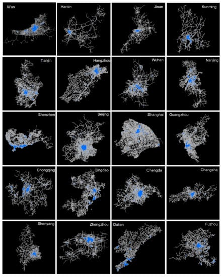
Figure 3.
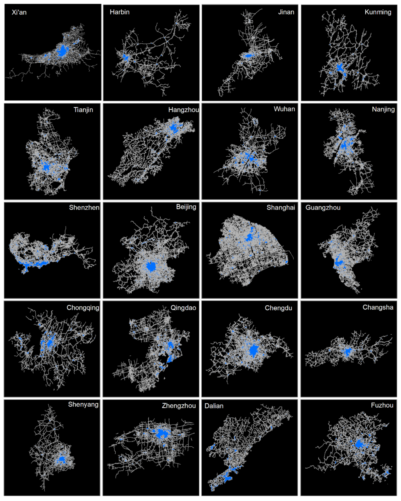
(Color online) Urban hotspots based on the density of street junctions throughout the top 20 Chinese cities.
2.3. Power Function Fitting for Intra-Urban Scaling Law Examination
The examination of urban scaling concerns two perspectives: The power law detection of a single urban indicator (as mentioned in Section 2.2.2) and the power relationship between two types of urban quantities (for example, urban areas versus populations). The latter have been formulated as the universal scaling law [16] for most of the urban indicators, which uses the power function fitting between an urban indicator and the urban population size across cities at time , denoted as Equation (6):
where is the scaling exponent and is the constant.
The scaling exponent can be further investigated by means of three categories: The sub-linear (), linear (), and super-linear () scaling relationships between urban measures [16]. To elaborate, for , it normally refers to the need of a city’s infrastructure scales sub-linearly with its population size due to the economies of scale, whereas the number of a city’s innovations and crimes scales super-linearly () due to the endogenous social interactions. The regime of describes the pattern that the individual demands in a city is proportionate to the urban population size. In this study, we use the detected hotspots as alternative spatial units to reexamine the urban scaling law. To do so, we conduct the power function fitting between urban socio-economic metrics (such as population, GDP, and CO2 emissions) that are within urban hotspots. To compute the scaling exponent, we first take the logarithms on both axes and adopt the ordinary least-squares linear regression for fitting. The scaling exponent is then the slope of the fitting line.
3. Results
3.1. Derived Urban Hotspots in the Top 20 Chinese Cities
We applied the urban hotspot detection method on street nodes and NTL imagery, respectively, across top 20 Chinese cities, ranked by GDP. To derive the hotspots from the street nodes, we established big TIN models for each city, whose TIN edges range from tens to hundreds of thousands (Table 1). The heavy-tailed distribution statistics were striking for each TIN model, as the average edge length (the mean length of is about 450 m) was classified effectively between short and long TIN edges according to their imbalanced ratios (around 80% versus 20%). The observation of 80/20 division, namely the scaling pattern of far more short TIN edges than long ones, objectively reveals the uneven spatial distribution of street node densities. The delineation of urban hotspots for each city was then conducted by grouping and converting those short edges into many different-sized hotspots. The area of resulting hotspots per city followed well with Zipf’s law, as the mean value of 20 cities’ power-law exponents was 2.01 (for more details of the basic statistics and related power-law metrics of hotspot size, see Section 3.2). Figure 3 presents the appearance of hotspots across selected cities, clearly showing that a few largest patches were located in the downtown and numerous smaller ones were spaced dispersedly in places other than the city center.

Table 1.
Statistics of street nodes, related triangulated irregular network (TIN) edges, and head/tail division results among 20 cities. (Note: #: Number; : Average edge length).
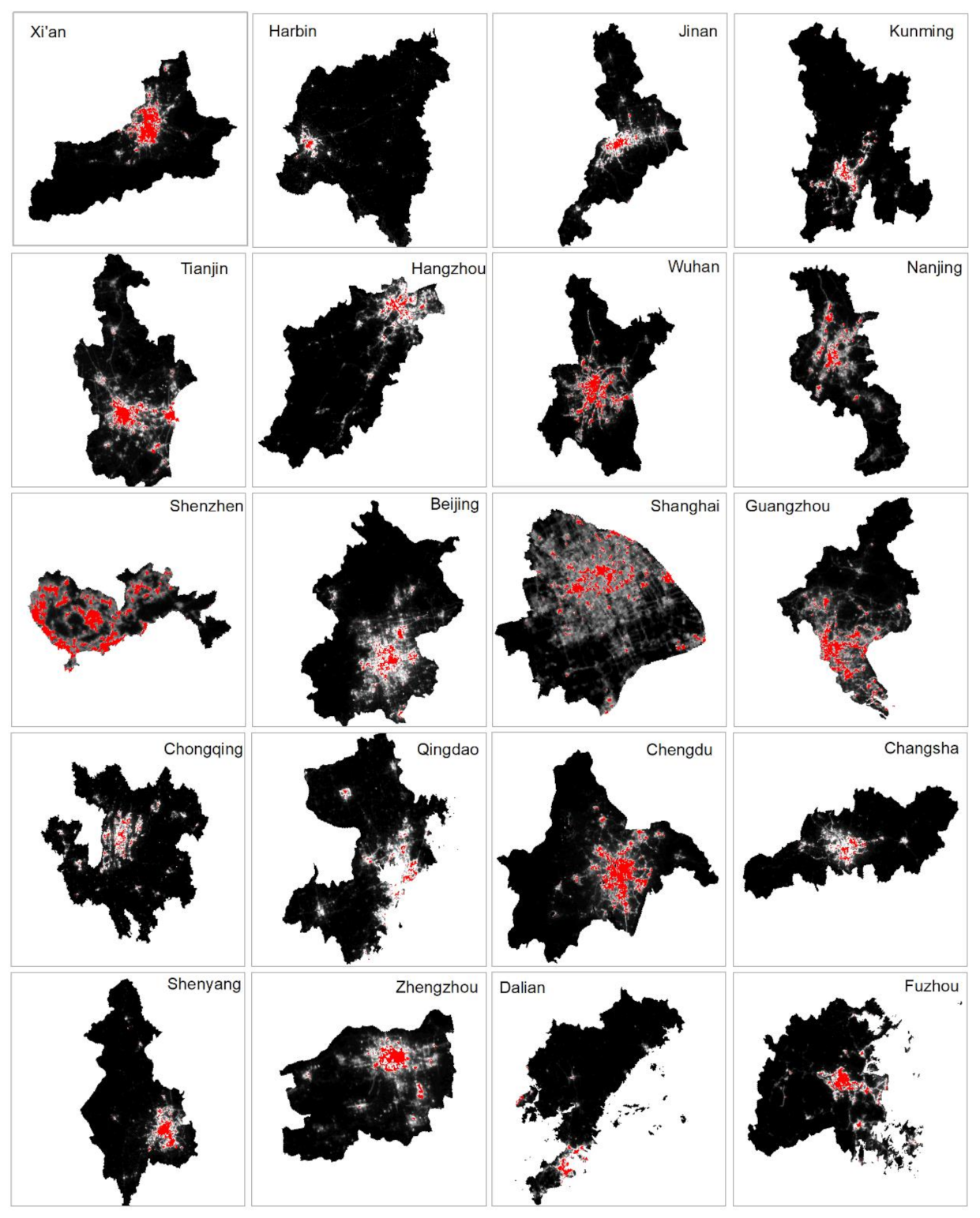
The urban hotspot extraction from NTL data went through experiments with a series of “candidate” mean values along with the head/tail breaking process on each image. To start with, the number of pixels for each image ranged widely, from 9397 (Shenzhen) to 353,344 (Harbin) and, interestingly, also followed the fat-tailed distribution. More specifically, among 20 city NTL images, most of the images (14) contain fewer than 78,045 pixels, some (five) between 78,045 and 141,623 pixels, while only one image has more than 141,623 pixels, resulting in a ht-index value of 3, meaning that there are three hierarchical levels of images regarding the number of pixels. Moreover, the ht-index for the pixel values of each city image was even higher. Figure 4 shows clearly that each image contains far more dark pixels than light ones, and such a scaling pattern recurs at least five times, indicating that there were no fewer than five average lightness values of each image achieved as candidate threshold values for a single city’s hotspot delineation (see Appendix A for more details of the head/tail breaks method applied to the pixel values of each city’s NTL data). Therefore, for every image we merged the vectorized pixels whose values above each derived candidate thresholds based on head/tail breaks to extract the urban hotspots, ensued with power law detection for each set of the hotspot results. The summary of statistical results for varying thresholds is presented in Table 2, which shows that the optimal cutoff value resided in the third level, since its power-law exponent was closest to 2, leading to hotspots being most akin to the Zipf’s law configuration. It should be noted that the average of the cutoff values across 20 cities (33.086) largely echoes the optimal threshold (33.14) based on the VIIRS NTL data in 2013 for Chinese city demarcation [35]. Following the located cutoffs for each image, the layout of extracted urban hotspots exhibited a picture that was overall similar to that from street nodes in terms of the imbalanced spatial distribution from city center to periphery (Figure 4).
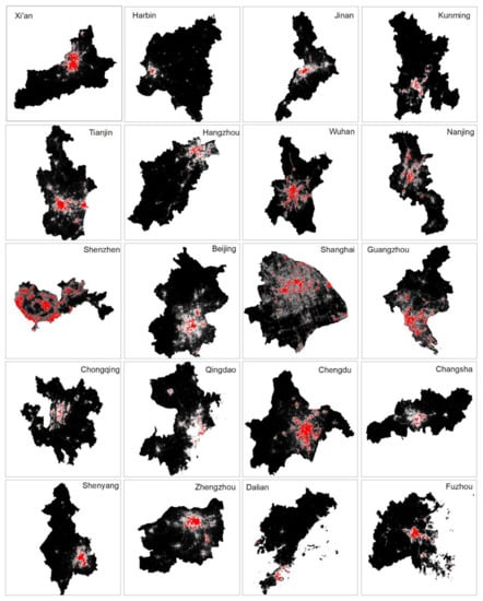
Figure 4.
(Color online) Urban hotspots based on NTL imagery using the third mean value as the cutoff value.

Table 2.
The candidate cutoff values for the NTL image and the resulting power law exponents at different levels based on the head/tail breaks method. (Note: : The average of lightness thresholds at each level for 20 images; : The average of power-law exponent of hotspot area for 20 cities).
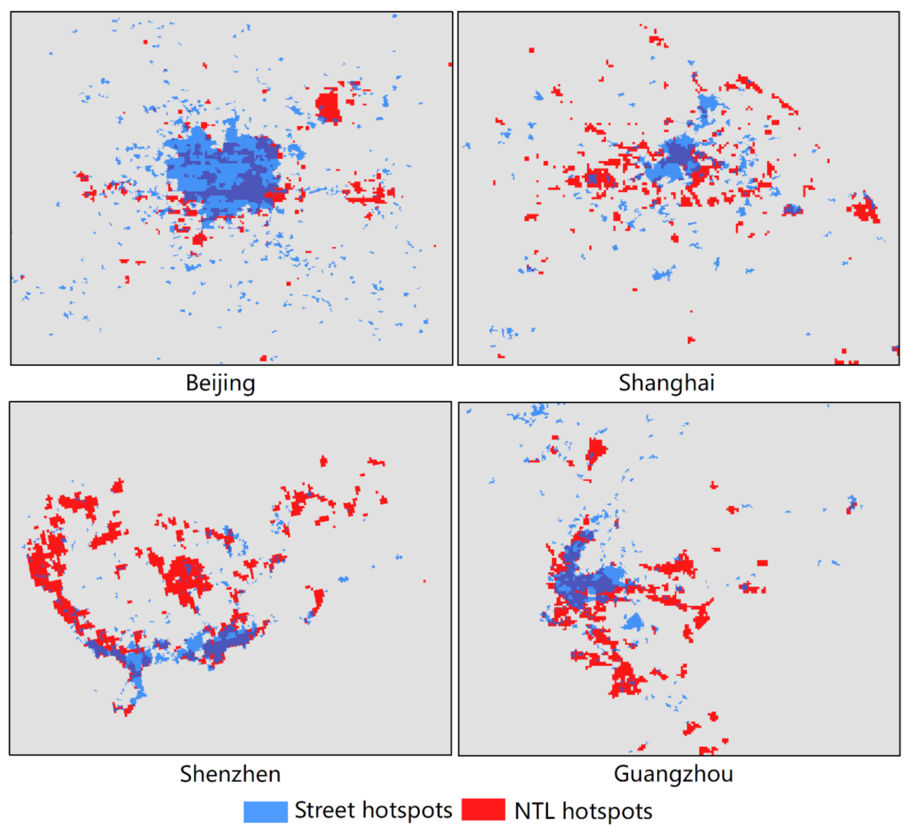
By comparing Figure 3 with Figure 4, it is clear that two types of patches overlapped, but in varying degrees, with each other, indicating there were similarities and differences between urban physical and functional extents. Here, we applied the intersection over union (IoU) metric to compute the overlapping ratio between two types of hotspots for each city, the average ratio for 20 cities was around 0.27 (see more details in Appendix B). It appeared that inland cities were inclined to have larger ratios, such as Shenyang, Xian, and Zhengzhou had most overlays (around 0.4), whereas coastal cities such as Shenzhen and Qingdao held much less (e.g., only 0.11 for Qingdao). We further opted to map the overlay between two types of hotspots among the top four representative cities in China: Beijing, Shanghai, Guangzhou, and Shenzhen (Figure 5), whose IoU metrics are all smaller than the average, i.e., 0.26, 0.17, 0.21, 0.18, respectively. Moreover, it is intriguing to note that detailed disparities can be found with respect to the extent of dispersive patches. In other words, with similar power-law exponents (around 2), the sizes of NTL hotspots in top cities seemed to be more even and the spatial distribution were more dispersed than those of street hotspots.

Figure 5.
(Color online) Comparison between two types of urban hotspots in four Chinese first-tier cities.
3.2. Intra-Urban Scaling Properties Based on Derived Urban Hotspots
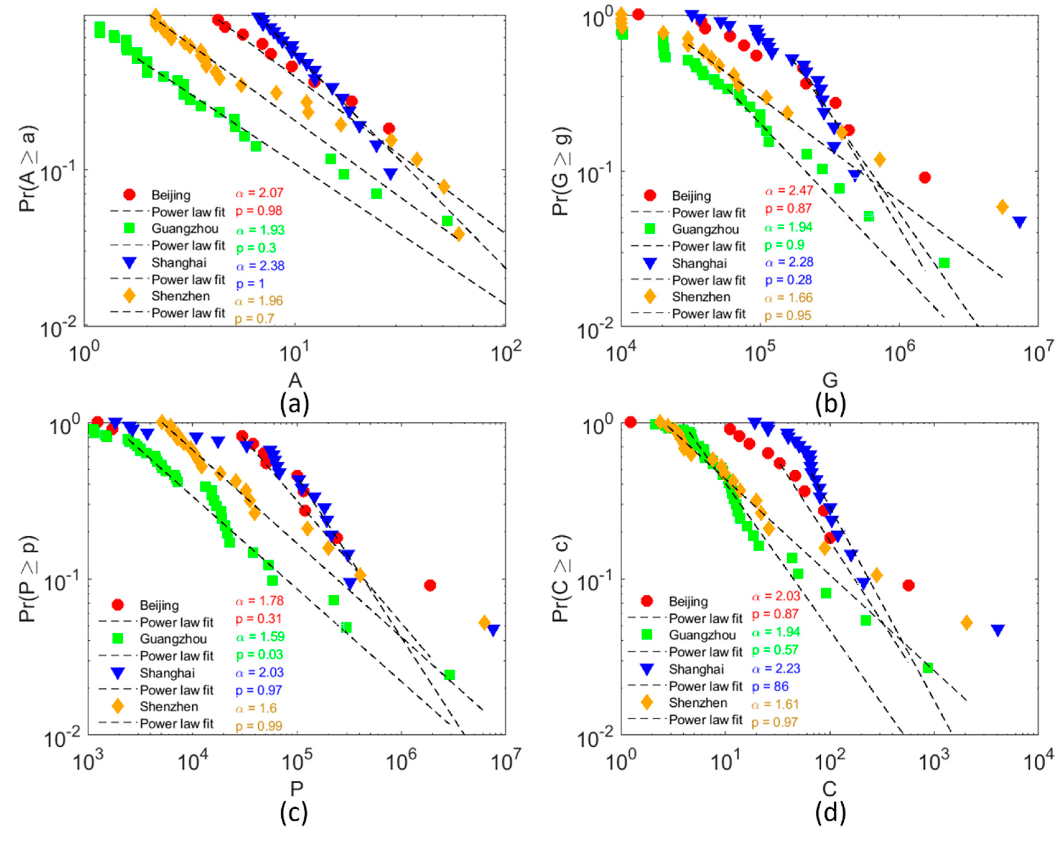
We applied the robust power law detection based on the MLE method to two types of hotspots in 20 cities. For each city, we listed the power-law fitting metrics regarding its hotspot areas detected using the cutoffs derived from head/tail breaks (Table 3). We can see that Zipf’s law held remarkably well for both types of urban hotspots. As stated, the power-law exponents for street hotspots were centered at 2.010.15, while the averaged exponent value for NTL hotspots was slightly smaller, 1.921 0.19, due to the exception of Chengdu (1.46). Most of the p-values were above 0.05 and readers can cross-check the results in Table 3. In addition to the hotspot sizes, we also examined the power law fit of the socio-economic status within the hotspots in the top four cities. As Figure 6 shows, the power-law distribution still holds for GDP, population, and the amount of CO2 emissions per hotspot, respectively. However, the values of exponents for each city performed slightly differently. Specifically, the exponents of three urban metrics inside the hotspots remained relatively stable with the hotspot size in Guangzhou and Shanghai, but less so in Beijing (up-and-downs around ) and Shenzhen (all smaller than ).

Table 3.
Power law metrics of detected urban hotspot areas. (Note: : Power-law exponent; : The goodness-of-fit index; : The minimum area above which the power-law holds).

Figure 6.
(Color online) Power law distribution of NTL-based hotspot sizes (a), GDP (b), population (c), and CO2 emissions (d) among the top four cities in China.
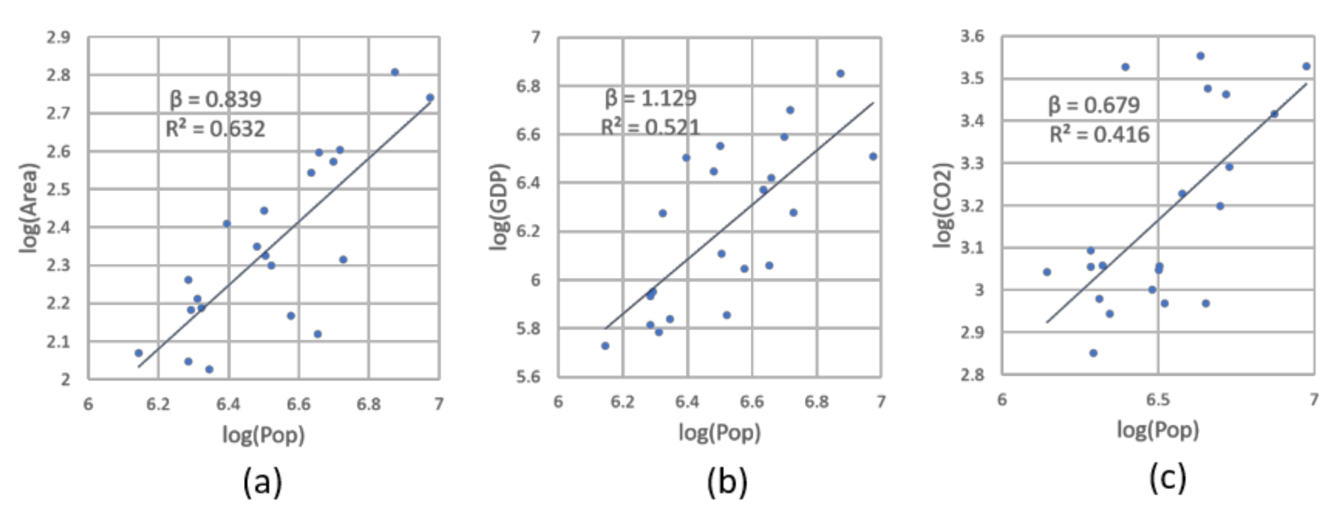
We further investigated how these extracted hotspots worked as cores of each city. Ideally, there should be a disproportionate relationship between hotspot areas and the amount of pertained resources. Consequently, 3% of the city area, constituting either type of hotspot, accommodates, on average, around 15% of GDP, 25% of population, and 20% of CO2 emissions (Table 4). Extreme cases such as Shenyang, Wuhan, and Kunming showed that derived hotspots could even account for more than 40% of the city’s total population or GDP. Such imbalanced ratios enabled us to make use of those urban indicators within the hotspots for exploring the intra-urban scaling law. After correlating the total areas, GDP, and CO2 emissions with the population, based on two types of hotspots for each city in double logarithm scales, we were intrigued by two findings. Firstly, there were no scaling relationships between the area/GDP/CO2 emissions and population based on the street hotspots, indicated by the very low R2 values (below 0.01), while significant scaling relationships existed when using NTL hotspots (R2 values above 0.4). Secondly, the relationships of area- and CO2 emissions-population were sub-linear (0.84 and 0.68; Figure 7a,c), whereas the GDP–population relationship was super-linear (1.13; Figure 7b), wherein the corresponding scaling exponent values, computed among the chosen 20 cities, were very consistent with values from the recent study based on 287 Chinese prefecture-level cities [17].

Table 4.
Percentages of area, gross domestic product (GDP), population, and CO2 emissions inside urban hotspots to those of the entire city. (Note: Pop: Population; CO2: CO2 emissions).
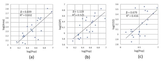
Figure 7.
(Color online) Scaling relations and exponents for urban indicators reflected by NTL-based hotspots (Note: Panels (a,c)show sub-linear scaling law for area/CO2 emissions versus population; Panel (b) shows super-linear scaling law of GDP and population; all metrics for each city are calculated based on the extent of contained NTL-based hotspots).
4. Discussion
Cities have long been treated as complex systems. The formation of cities can be described as a dynamic, self-organized, and nonlinear process of human settlements [5], demonstrating highly-heterogenous patterns in both its spatial and aspatial aspects [42]. The spatial aspect can refer to the fractal urban form and the aspatial aspect can refer to the long-tailed distribution of city-related metrics. However, such heterogeneities cannot be revealed effectively since conventional urban data, formed normally through top-down approaches, lack sufficient geographic scope and granularity. In the current geospatial big data era, we can easily conquer this constraint by acquiring fine-grained open data regarding the city form and function at countrywide coverage. Big data is not only big, but also possesses significant fractal and nonlinear properties [43], based on which we can model and analyze a city in a bottom-up manner. That is, delimiting city boundary at the country level or delineating hotspot area at the city scale by agglomeration of individual-based locations.
By adopting the fractal and nonlinear ways of thinking and doing, the cutoff for hotspot boundary derivation was located effectively. Specifically, drawing the border of hotspots is similar to measuring the length of a coastline—a commonality between the two is that, in reality, there is no ground truth for them. The father of fractal geometry, Benoit Mandelbrot [44], has made it clear that the length of a coastline is immeasurable, while the nonlinearity or scaling property is always measurable. In the present study, we characterized the data’s nonlinearity in its inherent scaling hierarchy (by head/tail breaks) and power-law or Zipf’s law distribution (by the MLE method), by which we obtained the cutoff guiding the spatial clustering. Taking the NTL image as an example, the nested mean values enable us to quickly classify pixels iteratively into a minority of light ones and a majority of dark ones, without exhausting all pixel values by increasing the threshold one at a time. Accordingly, only a few times of experiments on grouping-light-pixel operations for each city led us to generate hotspot polygons whose sizes follow Zipf’s law.
The successfully detected Zipf’s law of street- and NTL-based hotspots across 20 cities further strengthen the fractal structure of geographic space. It is well-known that a part of a fractal is similar geometrically or statistically to the whole, termed as self-similarity. Since there has been a good agreement among scholars that Zipf’s law holds for cities at the country scale [36,45], such a repeated statistical regularity for hotspots at the city scale in the present study can be considered evidence of the self-similarity of geographic space. The self-similarity across multiple scales makes us connect the system of geographic space with that of biology, where similar power law statistics appear across multiple layers in a human body from organs, to tissues, and further to cells [46,47]. Therefore, we believe that Zipf’s law can hold within even smaller sub-units than city hotspots (such as neighborhoods), and thus more refined urban center areas could be further identified with the proposed methods. This certainly warrants further study as long as the data granularity allows.
The detected hotspots in both types constituted only a small part of the city area, but accounted for a considerable portion of the urban population, wealth, and energy. This imbalanced ratio between hotspot sizes and the associated socio-economic statistics sheds light on the fact that not all city areas for people live or perform activities. This is also known as the potential problem of the administrative city boundary for urban analysis [21]. Without an accurate capture of human urban activities, the urban scaling estimations may be subjected to unexpected variations. We also examined the power relationship between selected urban measures within the entire administrative boundary among 20 cities, and failed to achieve expected scaling exponents (small R2 values or in wrong regimes), similar to the case when using the street-based hotspots. By contrast, through the NTL-based hotspots, the derived scaling relationships of area/GDP/CO2 to population were consistent with the established regimes (e.g., [17,48]). The obtained scaling exponents, shown in Figure 7, indicated that due to a more concentrated settlement and use of infrastructure, the growth of urban economy paced quicker than that of the population (super-linear regime), while the demands of urban areas and the related energy consumption accelerates slower than the population growth (sub-linear regime). The presence of scaling law further implied that the NTL-based hotspots could work as a new, effective instrument for exploring the system of cities.
The hotspots identified by both street and NTL data, by and large, tally with the locations of central urban areas of these 20 cities in China. As noted, street-based hotspots can represent a city’s morphological aspects, whereas NTL-based hotspots can accurately reflect a city’s functional aspects. The comparison between the two can give us a comprehensive image of how people utilized the urban space. It is noteworthy that the disparity occurs in their spatial distributions. Given that NTL-based hotspots illustrate the aggregation of human activities, we refer that the NTL-based hotspots better manifest the actual urban populous areas than the street-based hotspots, in the context that the street network constructed or traffic planning normally show a time lag. This discrepancy normally hints the evolution of urban centers. That is, these regions are preferred by humans, but apt to be neglected by the municipal authorities or urban scholars. Thus, the planning authorities should at least pay attention to these regions and other urban infrastructure should be strengthened in order to keep pace with real human needs, as well.
By computing IoU metrics, we are able to find that two types of hotspots have less overlays in coastal cities than in inland cities, while coastal cities in China normally have better economic status. Meanwhile, it is worth mentioning that the NTL-based hotspots are very dispersed in the four headmost metropolises, indicating that well-developed cities tend to exhibit a balanced distribution of human activities. It is further referred that cities with higher economic status shift to a more decentralized structure upon urban autonomous development. On this basis, the governments need to take more measures to promote urban justice (including the even distribution of urban resources, etc.) on the process of urban development.
5. Conclusions
The ultimate goal of city science is closely related to urban smart growth and sustainable development. In natural and societal phenomena, it has been widely adopted that the scaling pattern and power-law statistics are signs of sustainability [49]. This paper provides an intra-urban perspective to study the underlying scaling structure of urban space through novel spatial units: Urban hotspots, detected from geospatial big data including OSM street data and VIIRS imagery. In contrast to conventional spatial units that were imposed by local authorities, the present study adopted the objectively delineated concentration areas as hotspots using the spatial clustering approach. This is mainly motivated by the instability of urban scaling exponents affected by different cities and its sub-unit demarcations. In sum, we found (1) that Zipf’s law also holds strikingly at the intra-urban level; and (2) that NTL-based hotspots can be good proxies for city populous areas, by which the urban scaling relationship can be correctly maintained.
The method for hotspot detection acts as a promising tool and could supplement innovative urban planning toolboxes in the big data era. Despite the strengths of urban hotspot in this work, there is still room for improvement in terms of the following. Firstly, whether the intra-urban scaling law exists in other countries remains to be verified from a global view, in addition to these 20 cities in China. Secondly, it is important to add NTL images before 2020 to check whether and how the intra-urban scaling exponents change or evolve. Further, the updated raster data sets of GDP, population, and CO2 emissions after 2010 will be combined once they are available, for eliminating possible biases or inaccuracies that occurred due to the difference in data time acquisition. Thirdly, the multiscale effect of scaling analytics (e.g., detecting a more refined spatial unit and related power law statistics) within one city needs to be further conducted. Fourthly, the underlying mechanism of this scaling law has not been revealed yet, concerning policy, landform or demographic traits, etc. Future work will point to these directions.
Author Contributions
Conceptualization, D.M.; data curation, J.Y.; formal analysis, D.M. and Y.Z.; funding acquisition, D.M. and Z.Z.; methodology, D.M. and Y.J.; supervision, R.G. and Z.Z.; visualization, J.Y.; writing—original draft, D.M.; writing—review and editing, D.M. and Z.Z. All authors have read and agreed to the published version of the manuscript.
Funding
This research was financially supported by the National Nature Science Foundation of China (grant no. 42001180) and the China Postdoctoral Science Foundation (grant no. 2019M663038), and the National Key Research and Development Program of China [Grant No. 2018YFB2100705].
Data Availability Statement
Data sharing not applicable.
Acknowledgments
We would like to thank the anonymous referees and the editor for their constructive comments. We also would like to thank Chengyue Zhang, Wei Zhu, and Qionghuan Liu for their useful suggestions on NTL data acquisition and processing.
Conflicts of Interest
The authors declare no conflict of interest.
Appendix A
This appendix supplements Section 3.1 by showing average pixel values derived along with the head/tail breaks process of each nighttime image and the resulting power law metrics on hotspot sizes, by city.

Table A1.
The candidate cutoffs for spatial clustering of light pixels for hotspot detection and their corresponding power law metrics. (Note: NA: Not available; for most of cities, the number of scaling hierarchies of NTL image pixel lightness 5, meaning that there were at least 5 iteratively-averaged pixel values leading to an imbalanced ratio between dark-to-light pixels per city image. Among those five candidate cutoffs, the third one appeared to be the most suitable for urban hotspot delineation, as the almost related values of hotspot areas were closest to 2 and with an acceptable ).
| 1st Mean | 2nd Mean | 3rd Mean | 4th Mean | 5th Mean | |||||||||||
|---|---|---|---|---|---|---|---|---|---|---|---|---|---|---|---|
| Chengdu | 5.45 | 2.68 | 0.65 | 22.81 | 1.36 | 0.00 | 40.12 | 1.46 | 0.00 | 55.94 | 4.94 | 0.46 | 73.61 | 2.53 | 0.00 |
| Dalian | 1.65 | 1.69 | 0.27 | 12.74 | 1.67 | 0.97 | 32.90 | 1.70 | 0.11 | 57.31 | 3.66 | 0.72 | 101.36 | 13.52 | 0.69 |
| Fuzhou | 2.96 | 1.70 | 0.71 | 13.93 | 1.90 | 1.00 | 30.92 | 2.19 | 0.96 | 47.98 | 1.67 | 0.58 | 61.96 | 2.27 | 0.23 |
| Harbin | 0.42 | 1.62 | 0.05 | 3.81 | 1.93 | 0.92 | 17.64 | 1.93 | 0.74 | 35.20 | 1.88 | 0.24 | 52.37 | 1.58 | 0.01 |
| Hangzhou | 2.47 | 1.77 | 0.17 | 12.78 | 1.70 | 0.47 | 25.18 | 1.93 | 0.91 | 36.08 | 2.28 | 0.61 | 47.26 | NA | NA |
| Jinan | 2.86 | 1.80 | 0.93 | 12.93 | 1.77 | 0.71 | 24.88 | 2.17 | 0.94 | 35.18 | 2.61 | 0.89 | 44.83 | NA | NA |
| Kunming | 1.32 | 1.81 | 0.98 | 12.44 | 1.80 | 0.81 | 29.13 | 1.77 | 0.43 | 45.05 | 2.74 | 0.35 | 64.17 | 2.95 | 0.19 |
| Nanjing | 5.55 | 1.90 | 0.51 | 19.08 | 1.55 | 0.11 | 32.64 | 1.93 | 0.90 | 50.25 | 2.84 | 0.86 | 88.34 | 2.15 | 0.71 |
| Qingdao | 2.44 | 1.63 | 0.96 | 12.21 | 1.71 | 0.34 | 23.53 | 1.76 | 0.26 | 34.10 | 2.97 | 0.71 | 45.80 | NA | NA |
| Shanghai | 18.70 | 1.60 | 0.98 | 33.94 | 1.72 | 0.93 | 47.39 | 2.38 | 1.00 | 69.08 | 2.58 | 0.68 | 113.40 | 2.23 | 0.31 |
| Shenzhen | 25.28 | 1.57 | 0.60 | 46.04 | 1.61 | 0.97 | 61.94 | 1.96 | 0.94 | 76.91 | 1.61 | 0.70 | 96.40 | 2.18 | 0.42 |
| Shenyang | 2.36 | 1.89 | 0.85 | 16.90 | 1.89 | 0.15 | 34.82 | 1.89 | 0.27 | 50.86 | 1.93 | 0.96 | 66.10 | 1.98 | 0.98 |
| Tianjin | 5.58 | 1.72 | 0.75 | 18.98 | 1.72 | 0.91 | 32.71 | 1.80 | 0.63 | 44.99 | 2.32 | 0.88 | 59.59 | 1.97 | 0.21 |
| Wuhan | 5.28 | 2.15 | 0.01 | 22.72 | 2.00 | 0.88 | 40.42 | 1.73 | 0.07 | 58.95 | 2.40 | 1.00 | 81.18 | 2.55 | 0.86 |
| Xian | 3.72 | 1.70 | 1.00 | 22.12 | 1.88 | 0.14 | 40.78 | 1.88 | 0.80 | 54.78 | 1.74 | 0.21 | 70.79 | 2.51 | 0.85 |
| Changsha | 2.07 | 1.81 | 0.77 | 14.04 | 1.87 | 0.97 | 27.55 | 1.88 | 0.57 | 40.50 | 2.22 | 0.53 | 54.86 | 3.60 | 0.85 |
| Zhengzhou | 4.83 | 1.81 | 0.10 | 16.52 | 1.60 | 0.41 | 30.53 | 1.97 | 0.24 | 43.27 | 1.75 | 0.25 | 58.97 | 3.18 | 0.38 |
| Chongqing | 1.93 | 1.71 | 0.00 | 10.58 | 1.96 | 0.98 | 24.07 | 2.09 | 0.88 | 37.50 | 2.20 | 0.02 | 51.31 | 2.90 | 0.15 |
| Beijing | 4.33 | 1.73 | 0.84 | 16.23 | 1.83 | 1.00 | 27.75 | 2.07 | 0.98 | 37.95 | 1.94 | 0.91 | 52.87 | 2.07 | 0.94 |
| Guangzhou | 8.31 | 1.96 | 0.06 | 23.02 | 1.90 | 0.17 | 36.83 | 1.93 | 0.30 | 49.98 | 2.57 | 0.63 | 70.81 | 2.15 | 0.61 |
Appendix B
This appendix supplements Section 3.1 by presenting the overlapping ratios between street- and NTL-based hotspots among 20 cities. We adopted for assessing how much one type of hotspot overlaps another in a city. The metric between two types of hotspots can be denoted by the following equation:
where is the total area of street-based hotspots, is the total area of NTL-based hotspots. The results of for each city is shown in Table A2.

Table A2.
The intersection over union (IoU) metrics between two types of hotspots among 20 cities.
Table A2.
The intersection over union (IoU) metrics between two types of hotspots among 20 cities.
| City | IoU | City | IoU |
|---|---|---|---|
| Beijing | 0.26 | Nanjing | 0.19 |
| Shanghai | 0.17 | Changsha | 0.24 |
| Guangzhou | 0.21 | Zhengzhou | 0.38 |
| Shenzhen | 0.18 | Qingdao | 0.11 |
| Chengdu | 0.38 | Shenyang | 0.45 |
| Hangzhou | 0.28 | Dalian | 0.21 |
| Chongqing | 0.21 | Fuzhou | 0.33 |
| Wuhan | 0.22 | Harbin | 0.26 |
| Xian | 0.42 | Jinan | 0.34 |
| Tianjin | 0.33 | Kunming | 0.28 |
References
- United Nations. World Urbanization Prospects: The 2018 Revision; United Nations: New York, NY, USA, 2019. [Google Scholar]
- Zhao, S.; Zhou, D.; Zhu, C.; Sun, Y.; Wu, W.; Liu, S. Spatial and temporal dimensions of urban expansion in China. Environ. Sci. Technol. 2015, 49, 9600–9609. [Google Scholar] [CrossRef] [PubMed]
- National Bureau of Statistics. China Statistical Yearbook 2020; China Statistics Press: Beijing, China, 2020. [Google Scholar]
- Jacobs, J. The Death and Life of Great American Cities; Vintage Books: New York, NY, USA, 1961. [Google Scholar]
- Batty, M.; Longley, P. Fractal Cities: A Geometry of Form and Function; Academic Press: London, UK, 1994. [Google Scholar]
- Frankhauser, P. The fractal approach: A new tool for the spatial analysis of urban agglomerations. Popul. Engl. Sel. 1998, 10, 205–240. [Google Scholar]
- Batty, M. Cities and Complexity: Understanding Cities with Cellular Automata, Agent-Based Models, and Fractals; MIT Press: Cambridge, MA, USA, 2007. [Google Scholar]
- Chen, Y. Urban chaos and perplexing dynamics of urbanization. Lett. Spat. Resour. Sci. 2009, 2, 85–95. [Google Scholar] [CrossRef]
- Barthelemy, M. The Structure and Dynamics of Cities: Urban Data Analysis and Theoretical Modeling; Cambridge University Press: Cambridge, UK, 2016. [Google Scholar]
- Pumain, D.; Reuillon, R. Urban Dynamics and Simulation Models; Springer: Berlin, Germany, 2017. [Google Scholar]
- Shreevastava, A.; Rao, P.S.C.; McGrath, G.S. Emergent self-similarity and scaling properties of fractal intra-urban heat islets for diverse global cities. Phys. Rev. E 2019, 100, 032142. [Google Scholar] [CrossRef]
- Zipf, G. Human Behavior and the Principle of Least Effort; Addison-Wesley Press: Cambridge, MA, USA, 1949. [Google Scholar]
- Batty, M.; Carvalho, R.; Hudson-Smith, A.; Milton, R.; Smith, D.; Steadman, P. Scaling and allometry in the building geometries of Greater London. Eur. Phys. J. B 2008, 63, 303–314. [Google Scholar] [CrossRef]
- Carvalho, R.; Penn, A. Scaling and universality in the micro-structure of urban space. Phys. A Stat. Mech. Its Appl. 2004, 332, 539–547. [Google Scholar] [CrossRef]
- Jing, Y.; Liu, Y.; Cai, E.; Liu, Y.; Zhang, Y. Quantifying the spatiality of urban leisure venues in Wuhan, Central China—GIS-based spatial pattern metrics. Sustain. Cities Soc. 2018, 40, 638–647. [Google Scholar] [CrossRef]
- Bettencourt, L.M.A.; Lobo, J.; Helbing, D.; Kühnert, C.; West, G.B. Growth, innovation, scaling, and the pace of life in cities. Proc. Natl. Acad. Sci. USA 2007, 104, 7301–7306. [Google Scholar] [CrossRef]
- Zünd, D.; Bettencourt, L.M.A. Growth and development in prefecture-level cities in China. PLoS ONE 2019, 14, e0221017. [Google Scholar] [CrossRef]
- Lan, T.; Li, Z.; Zhang, H. Urban allometric scaling beneath structural fractality of road networks. Ann. Am. Assoc. Geogr. 2019, 109, 943–957. [Google Scholar] [CrossRef]
- Ma, D.; Guo, R.; Zheng, Y.; Zhao, Z.; He, F.; Zhu, W. Understanding Chinese Urban Form: The Universal Fractal Pattern of Street Networks over 298 Cities. ISPRS Int. J. Geo Inf. 2020, 9, 192. [Google Scholar] [CrossRef]
- Arcaute, E.; Hatna, E.; Ferguson, P.; Youn, H.; Johansson, A.; Batty, M. Constructing cities, deconstructing scaling laws. Interface 2015, 12, 20140745. [Google Scholar] [CrossRef]
- Alvioli, M. Administrative boundaries and urban areas in Italy: A perspective from scaling laws. Landsc. Urban Plan. 2020, 204, 103906. [Google Scholar] [CrossRef]
- Goodchild, M.F. Citizens as sensors: The world of volunteered geography. GeoJournal 2007, 69, 211–221. [Google Scholar] [CrossRef]
- Li, D.; Zhao, X.; Li, X. Remote sensing of human beings–a perspective from nighttime light. Geo Spat. Inf. Sci. 2016, 19, 69–79. [Google Scholar] [CrossRef]
- Bennett, J. Open Street Map: Be Your Own Cartographer; PCKT Publishing: Birmingham, AL, USA, 2010. [Google Scholar]
- Tannier, C.; Thomas, I.; Vuidel, G.; Frankhauser, P. A fractal approach to identifying urban boundaries. Geogr. Anal. 2011, 43, 211–227. [Google Scholar] [CrossRef]
- Tannier, C.; Thomas, I. Defining and characterizing urban boundaries: A fractal analysis of theoretical cities and Belgian cities. Comput. Environ. Urban Syst. 2013, 41, 234–248. [Google Scholar] [CrossRef]
- Long, Y.; Zhai, W.; Shen, Y.; Ye, X. Understanding uneven urban expansion with natural cities using open data. Landsc. Urban Plan. 2018, 177, 281–293. [Google Scholar] [CrossRef]
- Liu, L.; Xia, B.; Wu, H.; Zhao, J.; Peng, Z.; Yu, Y. Delimitating the natural city with points of interests based on service area and maximum entropy method. Entropy 2019, 21, 458. [Google Scholar] [CrossRef]
- Montero, G.; Tannier, C.; Thomas, I. Delineation of cities based on scaling properties of urban patterns: A comparison of three methods. Int. J. Geogr. Inf. Sci. 2021, 1–29. [Google Scholar] [CrossRef]
- Lynch, K. The Image of the City; MIT Press: Cambridge, MA, USA, 1960. [Google Scholar]
- NOAA/NCEI. Available online: http://data.mines.edu/nighttime_light/monthly/v10/2020/202006/ (accessed on 15 January 2021).
- Elvidge, C.D.; Baugh, K.; Zhizhin, M.; Hsu, F.C.; Ghosh, T. VIIRS night-time lights. Int. J. Remote Sens. 2017, 38, 5860–5879. [Google Scholar] [CrossRef]
- National Resources and Environment Database of the Chinese Academy of Sciences. Available online: http://www.resdc.cn/data.aspx?DATAID=252 (accessed on 15 January 2021).
- National Earth System Science Data Center. National Science and Technology Infrastructure of China. Available online: http://www.geodata.cn/data/datadetails.html?dataguid=49936583368636&docid=5173 (accessed on 15 January 2021).
- Wu, W.; Zhao, H.; Jiang, S. A Zipf’s Law-Based Method for Mapping Urban Areas Using NPP-VIIRS Nighttime Light Data. Remote Sens. 2018, 10, 130. [Google Scholar] [CrossRef]
- Newman, M.E.J. Power laws, Pareto distributions and Zipf’s law. Contemp. Phys. 2005, 46, 323–351. [Google Scholar] [CrossRef]
- Clauset, A.; Shalizi, C.; Newman, M. Power-law distributions in empirical data. Soc. Ind. Appl. Math. 2009, 51, 661–703. [Google Scholar] [CrossRef]
- Press, W.H.; William, H.; Teukolsky, S.A.; Saul, A.; Vetterling, W.T.; Flannery, B.P. Numerical Recipes 3rd Edition: The Art of Scientific Computing; Cambridge University Press: Cambridge, UK, 2007. [Google Scholar]
- Jiang, B. Head/tail breaks: A new classification scheme for data with a heavy-tailed distribution. Prof. Geogr. 2013, 65, 482–494. [Google Scholar] [CrossRef]
- Jiang, B.; Yin, J. Ht–index for quantifying the fractal or scaling structure of geographic features. Ann. Assoc. Am. Geogr. 2014, 104, 530–541. [Google Scholar] [CrossRef]
- Jiang, B.; Yin, J.; Liu, Q. Zipf’s law for all the natural cities around the world. Int. J. Geogr. Inf. Sci. 2015, 29, 498–522. [Google Scholar] [CrossRef]
- Stepinski, T.F.; Dmowska, A. Complexity in patterns of racial segregation. Chaos Solitons Fractals 2020, 140, 110207. [Google Scholar] [CrossRef]
- Li, S.; Dragicevic, S.; Castro, F.A.; Sester, M.; Winter, S.; Coltekin, A.; Pettit, C.; Jiang, B.; Haworth, J.; Stein, A.; et al. Geospatial big data handling theory and methods: A review and research challenges. ISPRS J. Photogramm. Remote Sens. 2016, 115, 119–133. [Google Scholar] [CrossRef]
- Mandelbrot, B. How long is the coast of Britain? Statistical self-similarity and fractional dimension. Science 1967, 156, 636–638. [Google Scholar] [CrossRef]
- Mitzenmacher, M. A brief history of generative models for power law and lognormal distributions. Internet Math. 2004, 1, 226–251. [Google Scholar] [CrossRef]
- García-Pérez, G.; Boguñá, M.; Serrano, M.Á. Multiscale unfolding of real networks by geometric renormalization. Nat. Phys. 2018, 14, 583–589. [Google Scholar] [CrossRef]
- Zheng, M.; Allard, A.; Hagmann, P.; Alemán-Gómez, Y.; Serrano, M.Á. Geometric renormalization unravels self-similarity of the multiscale human connectome. Proc. Natl. Acad. Sci. USA 2020, 117, 20244–20253. [Google Scholar] [CrossRef] [PubMed]
- Bettencourt, L.; West, G. A unified theory of urban living. Nature 2010, 467, 912–913. [Google Scholar] [CrossRef] [PubMed]
- Salat, S.; Bourdic, L. Urban complexity, scale hierarchy, energy efficiency and economic value creation. In The Sustainable City VII: Urban Regeneration and Sustainability; Pacetti, M., Passerini, G., Brebbia, C.A., Latini, G., Eds.; WIT Press: Boston, MA, USA, 2012; Volume 155, pp. 97–107. [Google Scholar]
Publisher’s Note: MDPI stays neutral with regard to jurisdictional claims in published maps and institutional affiliations. |
© 2021 by the authors. Licensee MDPI, Basel, Switzerland. This article is an open access article distributed under the terms and conditions of the Creative Commons Attribution (CC BY) license (https://creativecommons.org/licenses/by/4.0/).

