
Can Nighttime Satellite Imagery Inform Our Understanding of Education Inequality?


Abstract
1. Introduction
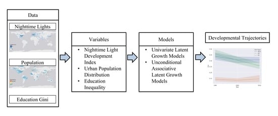
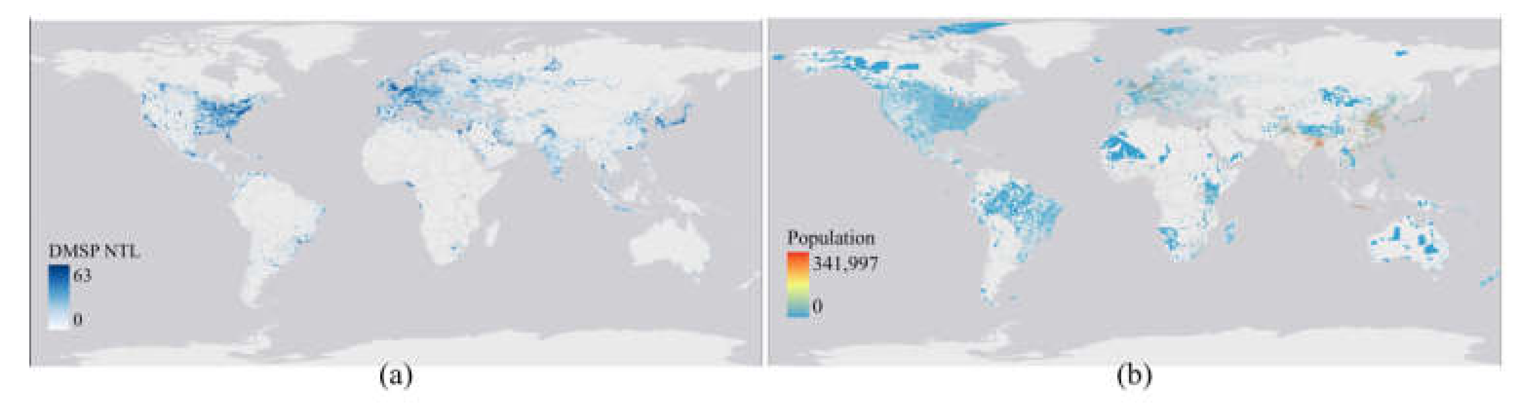
2. Data and Method
2.1. Gini Coefficients for Human Development and Education
2.2. Development of Associative Latent Growth Models (LGMs)
2.3. Latent Growth Model (LGM) Configuration Procedures
2.3.1. Unconditional Latent Growth Model (LGM) Specification for All Factors
2.3.2. Unconditional Three-Factor Associative Latent Growth Model (LGM)
2.3.3. Model Estimation and the Fit Indices
2.3.4. Model Parameter Estimation and Interpretation
3. Result
3.1. Model Configuration Results
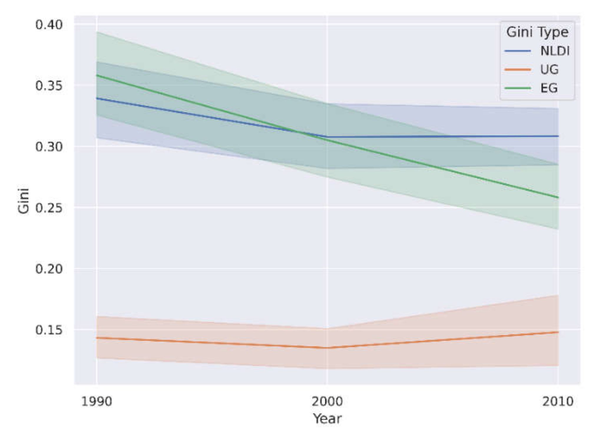
3.2. Associative Growth Trends
4. Discussion
5. Conclusions
Author Contributions
Funding
Conflicts of Interest
Appendix A

| Country | NLDI | Urban Population Gini | ||||
|---|---|---|---|---|---|---|
| 1990 | 2000 | 2010 | 1990 | 2000 | 2010 | |
| Afghanistan | 0.745 | 0.650 | 0.481 | 0.213 | 0.162 | 0.471 |
| Albania | 0.366 | 0.140 | 0.148 | 0.165 | 0.180 | 0.103 |
| United Arab Emirates | 0.225 | 0.341 | 0.339 | 0.055 | 0.054 | 0.018 |
| Argentina | 0.194 | 0.224 | 0.281 | 0.042 | 0.039 | 0.053 |
| Armenia | 0.242 | 0.240 | 0.333 | 0.143 | 0.154 | 0.084 |
| Australia | 0.101 | 0.145 | 0.143 | 0.036 | 0.031 | 0.013 |
| Austria | 0.233 | 0.241 | 0.248 | 0.231 | 0.225 | 0.008 |
| Burundi | 0.945 | 0.813 | 0.715 | 0.084 | 0.064 | 0.637 |
| Belgium | 0.104 | 0.118 | 0.153 | 0.061 | 0.065 | 0.003 |
| Benin | 0.446 | 0.366 | 0.415 | 0.158 | 0.125 | 0.323 |
| Bangladesh | 0.108 | 0.074 | 0.126 | 0.041 | 0.039 | 0.136 |
| Bulgaria | 0.201 | 0.174 | 0.198 | 0.148 | 0.184 | 0.047 |
| Bahrain | 0.447 | 0.478 | 0.577 | 0.030 | 0.021 | 0.033 |
| Belize | 0.196 | 0.178 | 0.213 | 0.136 | 0.141 | 0.096 |
| Bolivia | 0.326 | 0.251 | 0.240 | 0.046 | 0.036 | 0.090 |
| Brazil | 0.136 | 0.112 | 0.132 | 0.104 | 0.094 | 0.108 |
| Barbados | 0.180 | 0.186 | 0.296 | 0.174 | 0.158 | 0.048 |
| Brunei Darussalam | 0.056 | 0.109 | 0.216 | 0.146 | 0.136 | 0.008 |
| Botswana | 0.320 | 0.256 | 0.233 | 0.124 | 0.107 | 0.199 |
| Central African Republic | 0.751 | 0.681 | 0.506 | 0.209 | 0.190 | 0.614 |
| Canada | 0.277 | 0.289 | 0.342 | 0.076 | 0.067 | 0.011 |
| Switzerland | 0.192 | 0.226 | 0.230 | 0.123 | 0.115 | 0.016 |
| Chile | 0.221 | 0.276 | 0.289 | 0.063 | 0.061 | 0.064 |
| China | 0.336 | 0.264 | 0.262 | 0.068 | 0.072 | 0.130 |
| Cote d’Ivoire | 0.436 | 0.249 | 0.301 | 0.178 | 0.156 | 0.237 |
| Cameroon | 0.446 | 0.403 | 0.383 | 0.075 | 0.073 | 0.281 |
| Congo, Rep. | 0.456 | 0.402 | 0.719 | 0.120 | 0.127 | 0.267 |
| Colombia | 0.179 | 0.196 | 0.220 | 0.036 | 0.035 | 0.087 |
| Costa Rica | 0.157 | 0.256 | 0.318 | 0.136 | 0.120 | 0.029 |
| Cuba | 0.195 | 0.268 | 0.241 | 0.065 | 0.069 | 0.067 |
| Cyprus | 0.140 | 0.135 | 0.148 | 0.106 | 0.082 | 0.032 |
| Czech Republic | 0.159 | 0.185 | 0.208 | 0.147 | 0.155 | 0.011 |
| Germany | 0.117 | 0.166 | 0.208 | 0.113 | 0.112 | 0.007 |
| Denmark | 0.141 | 0.200 | 0.247 | 0.158 | 0.163 | 0.006 |
| Dominican Republic | 0.300 | 0.302 | 0.257 | 0.108 | 0.096 | 0.065 |
| Algeria | 0.594 | 0.496 | 0.376 | 0.095 | 0.076 | 0.059 |
| Ecuador | 0.281 | 0.227 | 0.235 | 0.113 | 0.102 | 0.096 |
| Egypt, Arab Rep. | 0.299 | 0.306 | 0.349 | 0.041 | 0.033 | 0.013 |
| Spain | 0.147 | 0.223 | 0.256 | 0.093 | 0.096 | 0.016 |
| Estonia | 0.311 | 0.190 | 0.254 | 0.180 | 0.195 | 0.040 |
| Finland | 0.166 | 0.214 | 0.208 | 0.109 | 0.110 | 0.018 |
| Fiji | 0.314 | 0.180 | 0.260 | 0.480 | 0.453 | 0.128 |
| France | 0.143 | 0.180 | 0.199 | 0.151 | 0.158 | 0.013 |
| Gabon | 0.691 | 0.723 | 0.616 | 0.138 | 0.129 | 0.177 |
| United Kingdom | 0.052 | 0.082 | 0.119 | 0.018 | 0.019 | 0.003 |
| Ghana | 0.388 | 0.234 | 0.215 | 0.116 | 0.090 | 0.276 |
| Gambia, The | 0.547 | 0.392 | 0.368 | 0.270 | 0.193 | 0.429 |
| Greece | 0.212 | 0.284 | 0.282 | 0.174 | 0.170 | 0.027 |
| Guatemala | 0.355 | 0.199 | 0.203 | 0.091 | 0.088 | 0.121 |
| Guyana | 0.418 | 0.301 | 0.309 | 0.205 | 0.188 | 0.210 |
| Hong Kong SAR, China | 0.493 | 0.512 | 0.505 | 0.007 | 0.006 | 0.118 |
| Honduras | 0.408 | 0.280 | 0.164 | 0.289 | 0.273 | 0.142 |
| Croatia | 0.242 | 0.192 | 0.245 | 0.197 | 0.212 | 0.048 |
| Haiti | 0.415 | 0.415 | 0.314 | 0.107 | 0.081 | 0.279 |
| Hungary | 0.163 | 0.150 | 0.207 | 0.162 | 0.171 | 0.046 |
| Indonesia | 0.335 | 0.224 | 0.245 | 0.072 | 0.076 | 0.147 |
| India | 0.313 | 0.323 | 0.338 | 0.064 | 0.057 | 0.124 |
| Ireland | 0.258 | 0.289 | 0.313 | 0.322 | 0.322 | 0.028 |
| Iran, Islamic Rep. | 0.519 | 0.327 | 0.295 | 0.061 | 0.049 | 0.032 |
| Iraq | 0.387 | 0.454 | 0.443 | 0.043 | 0.038 | 0.050 |
| Iceland | 0.297 | 0.464 | 0.570 | 0.354 | 0.289 | 0.071 |
| Israel | 0.371 | 0.425 | 0.446 | 0.067 | 0.054 | 0.020 |
| Italy | 0.130 | 0.159 | 0.176 | 0.099 | 0.094 | 0.006 |
| Jamaica | 0.120 | 0.192 | 0.201 | 0.105 | 0.097 | 0.018 |
| Jordan | 0.235 | 0.303 | 0.348 | 0.102 | 0.075 | 0.023 |
| Japan | 0.295 | 0.367 | 0.398 | 0.051 | 0.054 | 0.010 |
| Kazakhstan | 0.296 | 0.410 | 0.300 | 0.055 | 0.050 | 0.074 |
| Kenya | 0.639 | 0.523 | 0.544 | 0.378 | 0.319 | 0.508 |
| Kyrgyz Republic | 0.312 | 0.260 | 0.251 | 0.114 | 0.111 | 0.046 |
| Cambodia | 0.705 | 0.672 | 0.521 | 0.230 | 0.193 | 0.469 |
| Korea, Rep. | 0.417 | 0.465 | 0.499 | 0.080 | 0.075 | 0.015 |
| Kuwait | 0.593 | 0.637 | 0.665 | 0.030 | 0.035 | 0.013 |
| Lao PDR | 0.769 | 0.569 | 0.386 | 0.567 | 0.519 | 0.389 |
| Liberia | 0.663 | 0.599 | 0.421 | 0.352 | 0.328 | 0.555 |
| Libya | 0.645 | 0.483 | 0.458 | 0.095 | 0.094 | 0.037 |
| Sri Lanka | 0.208 | 0.194 | 0.218 | 0.389 | 0.362 | 0.049 |
| Lesotho | 0.414 | 0.392 | 0.330 | 0.170 | 0.178 | 0.246 |
| Lithuania | 0.110 | 0.060 | 0.111 | 0.049 | 0.060 | 0.033 |
| Luxembourg | 0.143 | 0.159 | 0.234 | 0.179 | 0.188 | 0.007 |
| Latvia | 0.064 | 0.140 | 0.148 | 0.096 | 0.108 | 0.057 |
| Macao | 0.419 | 0.431 | 0.518 | 0.003 | 0.002 | 0.013 |
| Morocco | 0.169 | 0.188 | 0.190 | 0.114 | 0.109 | 0.063 |
| Moldova | 0.274 | 0.214 | 0.194 | 0.228 | 0.244 | 0.127 |
| Mexico | 0.209 | 0.212 | 0.222 | 0.138 | 0.120 | 0.029 |
| Mali | 0.593 | 0.362 | 0.247 | 0.140 | 0.135 | 0.388 |
| Malta | 0.344 | 0.340 | 0.345 | 0.039 | 0.036 | 0.042 |
| Myanmar | 0.550 | 0.328 | 0.353 | 0.132 | 0.122 | 0.280 |
| Mongolia | 0.523 | 0.466 | 0.352 | 0.247 | 0.277 | 0.356 |
| Mozambique | 0.515 | 0.478 | 0.443 | 0.121 | 0.112 | 0.392 |
| Mauritania | 0.761 | 0.647 | 0.635 | 0.304 | 0.244 | 0.541 |
| Mauritius | 0.220 | 0.228 | 0.261 | 0.134 | 0.122 | 0.033 |
| Malawi | 0.531 | 0.437 | 0.370 | 0.569 | 0.545 | 0.420 |
| Malaysia | 0.181 | 0.232 | 0.248 | 0.097 | 0.089 | 0.063 |
| Namibia | 0.587 | 0.464 | 0.431 | 0.620 | 0.531 | 0.361 |
| Niger | 0.595 | 0.458 | 0.432 | 0.153 | 0.155 | 0.434 |
| Nicaragua | 0.393 | 0.247 | 0.237 | 0.056 | 0.055 | 0.254 |
| Netherlands | 0.152 | 0.167 | 0.225 | 0.081 | 0.082 | 0.010 |
| Norway | 0.331 | 0.347 | 0.341 | 0.209 | 0.211 | 0.028 |
| Nepal | 0.326 | 0.276 | 0.133 | 0.086 | 0.173 | 0.196 |
| New Zealand | 0.140 | 0.178 | 0.206 | 0.155 | 0.144 | 0.058 |
| Pakistan | 0.082 | 0.054 | 0.088 | 0.086 | 0.062 | 0.065 |
| Panama | 0.274 | 0.195 | 0.232 | 0.263 | 0.234 | 0.150 |
| Peru | 0.281 | 0.288 | 0.317 | 0.142 | 0.134 | 0.199 |
| Philippines | 0.497 | 0.374 | 0.314 | 0.315 | 0.295 | 0.206 |
| Papua New Guinea | 0.580 | 0.529 | 0.467 | 0.151 | 0.133 | 0.538 |
| Poland | 0.126 | 0.085 | 0.124 | 0.098 | 0.098 | 0.011 |
| Portugal | 0.215 | 0.295 | 0.325 | 0.226 | 0.215 | 0.019 |
| Paraguay | 0.294 | 0.198 | 0.220 | 0.139 | 0.148 | 0.176 |
| Qatar | 0.463 | 0.447 | 0.588 | 0.117 | 0.091 | 0.021 |
| Russian Federation | 0.346 | 0.359 | 0.412 | 0.058 | 0.063 | 0.061 |
| Rwanda | 0.820 | 0.696 | 0.641 | 0.064 | 0.079 | 0.486 |
| Saudi Arabia | 0.222 | 0.162 | 0.215 | 0.038 | 0.039 | 0.021 |
| Sudan | 0.506 | 0.467 | 0.427 | 0.059 | 0.050 | 0.401 |
| Senegal | 0.368 | 0.292 | 0.308 | 0.109 | 0.100 | 0.373 |
| Singapore | 0.224 | 0.189 | 0.210 | 0.001 | 0.001 | 0.025 |
| Sierra Leone | 0.503 | 0.534 | 0.479 | 0.216 | 0.198 | 0.556 |
| El Salvador | 0.237 | 0.166 | 0.156 | 0.098 | 0.092 | 0.041 |
| Serbia | 0.150 | 0.153 | 0.172 | 0.130 | 0.133 | 0.051 |
| Slovak Republic | 0.136 | 0.071 | 0.107 | 0.081 | 0.082 | 0.039 |
| Slovenia | 0.102 | 0.108 | 0.135 | 0.201 | 0.212 | 0.025 |
| Sweden | 0.279 | 0.341 | 0.313 | 0.125 | 0.134 | 0.011 |
| Eswatini | 0.202 | 0.168 | 0.115 | 0.219 | 0.179 | 0.156 |
| Syrian Arab Republic | 0.504 | 0.316 | 0.222 | 0.103 | 0.087 | 0.045 |
| Togo | 0.388 | 0.366 | 0.374 | 0.090 | 0.075 | 0.303 |
| Thailand | 0.496 | 0.358 | 0.294 | 0.234 | 0.232 | 0.124 |
| Tajikistan | 0.125 | 0.135 | 0.094 | 0.060 | 0.048 | 0.061 |
| Tonga | 0.338 | 0.112 | 0.111 | 0.279 | 0.318 | 0.099 |
| Trinidad and Tobago | 0.220 | 0.225 | 0.328 | 0.093 | 0.091 | 0.051 |
| Tunisia | 0.302 | 0.249 | 0.248 | 0.060 | 0.062 | 0.051 |
| Turkey | 0.265 | 0.288 | 0.221 | 0.122 | 0.116 | 0.087 |
| Tanzania | 0.575 | 0.491 | 0.407 | 0.197 | 0.182 | 0.499 |
| Uganda | 0.845 | 0.726 | 0.703 | 0.180 | 0.133 | 0.634 |
| Ukraine | 0.183 | 0.255 | 0.192 | 0.101 | 0.105 | 0.061 |
| Uruguay | 0.283 | 0.345 | 0.377 | 0.114 | 0.087 | 0.063 |
| United States | 0.204 | 0.259 | 0.279 | 0.142 | 0.128 | 0.005 |
| Venezuela, RB | 0.237 | 0.293 | 0.320 | 0.044 | 0.037 | 0.040 |
| Vietnam | 0.488 | 0.285 | 0.251 | 0.078 | 0.084 | 0.111 |
| Yemen, Rep. | 0.534 | 0.508 | 0.509 | 0.174 | 0.145 | 0.165 |
| South Africa | 0.269 | 0.190 | 0.187 | 0.237 | 0.191 | 0.110 |
| Zambia | 0.576 | 0.454 | 0.393 | 0.062 | 0.070 | 0.450 |
| Zimbabwe | 0.324 | 0.194 | 0.311 | 0.196 | 0.196 | 0.479 |
References
- Uited Nations. The 17 Goals—Sustainable Development. Available online: https://sdgs.un.org/goals (accessed on 21 June 2020).
- United Nations. Transforming Our World: The 2030 Agenda for Sustainable Development. 2015. Available online: https://sdgs.un.org/2030agenda (accessed on 10 June 2020).
- Griggs, D.; Stafford-Smith, M.; Gaffney, O.; Rockström, J.; Öhman, M.C.; Shyamsundar, P.; Steffen, W.; Glaser, G.; Kanie, N.; Noble, I. Policy: Sustainable Development Goals for People and Planet. Nature 2013, 495, 305. [Google Scholar] [CrossRef] [PubMed]
- Robert, K.W.; Parris, T.M.; Leiserowitz, A.A. What Is Sustainable Development? Goals, Indicators, Values, and Practice. Environ. Sci. Policy Sustain. Dev. 2005, 47, 8–21. [Google Scholar] [CrossRef]
- Sachs, J.D. From Millennium Development Goals to Sustainable Development Goals. Lancet 2012, 379, 2206–2211. [Google Scholar] [CrossRef]
- Thomas, V.; Wang, Y.; Fan, X. Measuring Education Inequality: Gini Coefficients of Education; The World Bank: Washington, DC, USA, 1999. [Google Scholar]
- Aghion, P.; Askenazy, P.; Bourlès, R.; Cette, G.; Dromel, N. Education, Market Rigidities and Growth. Econ. Lett. 2009, 102, 62–65. [Google Scholar] [CrossRef]
- Chen, M.; Zhang, H.; Liu, W.; Zhang, W. The Global Pattern of Urbanization and Economic Growth: Evidence from the Last Three Decades. PLoS ONE 2014, 9, e103799. [Google Scholar] [CrossRef]
- Hanushek, E.A.; Woessmann, L. Education and Economic Growth. In Economy of Education; Elsevier: Amsterdam, The Netherlands, 2010; pp. 60–67. [Google Scholar]
- Brown, P.H.; Park, A. Education and Poverty in Rural China. Econ. Educ. Rev. 2002, 21, 523–541. [Google Scholar] [CrossRef]
- Ladd, H.F. Education and Poverty: Confronting the Evidence. J. Policy Anal. Manag. 2012, 31, 203–227. [Google Scholar] [CrossRef]
- Place, K.; Hodge, S.R. Social Inclusion of Students with Physical Disabilities in General Physical Education: A Behavioral Analysis. Adapt. Phys. Act. Q. 2001, 18, 389–404. [Google Scholar] [CrossRef]
- Nilsson, A. Vocational Education and Training–an Engine for Economic Growth and a Vehicle for Social Inclusion? Int. J. Train. Dev. 2010, 14, 251–272. [Google Scholar] [CrossRef]
- Michalos, A.C.; Creech, H.; McDonald, C.; Kahlke, P.M.H. Knowledge, Attitudes and Behaviours. Concerning Education for Sustainable Development: Two Exploratory Studies. Soc. Indic. Res. 2011, 100, 391–413. [Google Scholar] [CrossRef]
- Singhal, A.; Sahu, S.; Chattopadhyay, S.; Mukherjee, A.; Bhanja, S.N. Using Night Time Lights to Find Regional Inequality in India and Its Relationship with Economic Development. PLoS ONE 2020, 15, e0241907. [Google Scholar] [CrossRef]
- Wu, R.; Yang, D.; Dong, J.; Zhang, L.; Xia, F. Regional Inequality in China Based on NPP-VIIRS Night-Time Light Imagery. Remote Sens. 2018, 10, 240. [Google Scholar] [CrossRef]
- Ivan, K.; Holobâcă, I.-H.; Benedek, J.; Török, I. Potential of Night-Time Lights to Measure Regional Inequality. Remote Sens. 2020, 12, 33. [Google Scholar] [CrossRef]
- Wang, X.; Rafa, M.; Moyer, J.D.; Li, J.; Scheer, J.; Sutton, P. Estimation and Mapping of Sub-National GDP in Uganda Using NPP-VIIRS Imagery. Remote Sens. 2019, 11, 163. [Google Scholar] [CrossRef]
- Dai, Z.; Hu, Y.; Zhao, G. The Suitability of Different Nighttime Light Data for GDP Estimation at Different Spatial Scales and Regional Levels. Sustainability 2017, 9, 305. [Google Scholar] [CrossRef]
- Wang, Y.; Huang, C.; Zhao, M.; Hou, J.; Zhang, Y.; Gu, J. Mapping the Population Density in Mainland China Using NPP/VIIRS and Points-Of-Interest Data Based on a Random Forests Model. Remote Sens. 2020, 12, 3645. [Google Scholar] [CrossRef]
- Elvidge, C.D.; Baugh, K.E.; Anderson, S.J.; Sutton, P.C.; Ghosh, T. The Night Light Development Index (NLDI): A Spatially Explicit Measure of Human Development from Satellite Data. Soc. Geogr. 2012, 7, 23–35. [Google Scholar] [CrossRef]
- Skinner, C. Issues and Challenges in Census Taking. Annu. Rev. Stat. Appl. 2018, 5, 49–63. [Google Scholar] [CrossRef]
- Doll, C.H.; Muller, J.-P.; Elvidge, C.D. Night-Time Imagery as a Tool for Global Mapping of Socioeconomic Parameters and Greenhouse Gas Emissions. AMBIO J. Hum. Environ. 2000, 29, 157–163. [Google Scholar] [CrossRef]
- Zhang, Q.; Seto, K.C. Mapping Urbanization Dynamics at Regional and Global Scales Using Multi-Temporal DMSP/OLS Nighttime Light Data. Remote Sens. Environ. 2011, 115, 2320–2329. [Google Scholar] [CrossRef]
- Baugh, K.; Elvidge, C.D.; Ghosh, T.; Ziskin, D. Development of a 2009 Stable Lights Product Using DMSP-OLS Data. Proc. Asia Pac. Adv. Netw. 2010, 30, 114–130. [Google Scholar] [CrossRef]
- Elvidge, C.D.; Baugh, K.E.; Dietz, J.B.; Bland, T.; Sutton, P.C.; Kroehl, H.W. Radiance Calibration of DMSP-OLS Low-Light Imaging Data of Human Settlements. Remote Sens. Environ. 1999, 68, 77–88. [Google Scholar] [CrossRef]
- Sutton, P.C.; Costanza, R. Global Estimates of Market and Non-Market Values Derived from Nighttime Satellite Imagery, Land Cover, and Ecosystem Service Valuation. Ecol. Econ. 2002, 41, 509–527. [Google Scholar] [CrossRef]
- Elvidge, C.D.; Sutton, P.C.; Ghosh, T.; Tuttle, B.T.; Baugh, K.E.; Bhaduri, B.; Bright, E. A Global Poverty Map Derived from Satellite Data. Comput. Geosci. 2009, 35, 1652–1660. [Google Scholar] [CrossRef]
- Song, Y.; Qiu, Q.; Guo, Q.; Lin, J.; Li, F.; Yu, Y.; Li, X.; Tang, L. The Application of Spatial Lorenz Curve (SLC) and Gini Coefficient in Measuring Land Use Structure Change. In Proceedings of the 18th International Conference on Geoinformatics, Beijing, China, 18–20 June 2010; pp. 1–5. [Google Scholar]
- Black, D.; Henderson, V. A Theory of Urban Growth. J. Political Econ. 1999, 107, 252–284. [Google Scholar] [CrossRef]
- Ciccone, A.; Hall, R.E. Productivity and the Density of Economic Activity; National Bureau of Economic Research: Cambridge, MA, USA, 1993. [Google Scholar]
- Montgomery, M.R.; Stren, R.; Cohen, B.; Reed, H.E. Cities Transformed: Demographic Change and Its Implications in the Developing World; Routledge: London, UK, 2013. [Google Scholar]
- Ziesemer, T. Gini Coefficients of Education for 146 Countries, 1950–2010. Bull. Appl. Econ. 2016, 3, 1–8. [Google Scholar]
- Hamilton, J.; Gagne, P.E.; Hancock, G.R. The Effect of Sample Size on Latent Growth Models. In Proceedings of the 2003 Meeting of the National Council on Measurement in Education, Chicago, IL, USA, 21–25 April 2003. [Google Scholar]
- Biglan, A.; Duncan, T.E.; Ary, D.V.; Smolkowski, K. Peer and Parental Influences on Adolescent Tobacco Use. J. Behav. Med. 1995, 18, 315–330. [Google Scholar] [CrossRef]
- Rogosa, D.; Brandt, D.; Zimowski, M. A Growth Curve Approach to the Measurement of Change. Psychol. Bull. 1982, 92, 726. [Google Scholar] [CrossRef]
- Stoolmiller, M. Using Latent Growth Curve Models to Study Developmental Processes. In The Analysis of Change; Erlbaum: Mahwah, NJ, USA, 1995; pp. 103–138. [Google Scholar]
- Tisak, J.; Meredith, W. Longitudinal factor analysis. In Statistical Methods in Longitudinal Research; Elsevier: Amsterdam, The Netherlands, 1990; pp. 125–149. [Google Scholar]
- Hox, J.J.; Kreft, I.G. Multilevel Analysis Methods. Sociol. Methods Res. 1994, 22, 283–299. [Google Scholar] [CrossRef]
- Curran, P.J.; Stice, E.; Chassin, L. The Relation between Adolescent Alcohol Use and Peer Alcohol Use: A Longitudinal Random Coefficients Model. J. Consult. Clin. Psychol. 1997, 65, 130. [Google Scholar] [CrossRef] [PubMed]
- Ge, X.; Lorenz, F.O.; Conger, R.D.; Elder, G.H.; Simons, R.L. Trajectories of Stressful Life Events and Depressive Symptoms during Adolescence. Dev. Psychol. 1994, 30, 467. [Google Scholar] [CrossRef]
- Wickrama, K.A.S.; Lorenz, F.O.; Conger, R.D.; Elder, G.H., Jr. Marital Quality and Physical Illness: A Latent Growth Curve Analysis. J. Marriage Fam. 1997, 59, 143–155. [Google Scholar] [CrossRef]
- Muthén, B.O.; Curran, P.J. General Longitudinal Modeling of Individual Differences in Experimental Designs: A Latent Variable Framework for Analysis and Power Estimation. Psychol. Methods 1997, 2, 371. [Google Scholar] [CrossRef]
- Muthén, L.K.; Muthén, B. Mplus. In The Comprehensive Modelling Program for Applied Researchers: User’s Guide; Muthén & Muthén: Los Angeles, CA, USA, 2018; p. 5. [Google Scholar]
- Bollen Kenneth, A.; Curran Patrick, J. Latent Curve Models: A Structural Equation Approach; Wiley: New York, NY, USA, 2005. [Google Scholar]
- Hooper, D.; Coughlan, J.; Mullen, M.R. Structural Equation Modelling: Guidelines for Determining Model Fit. Electron. J. Bus. Res. Methods 2008, 6, 53–60. [Google Scholar]
- MacCallum, R.C.; Browne, M.W.; Sugawara, H.M. Power Analysis and Determination of Sample Size for Covariance Structure Modeling. Psychol. Methods 1996, 1, 130. [Google Scholar] [CrossRef]
- Jöreskog, K.G.; Sörbom, D. LISREL 8: User’s Reference Guide; Scientific Software International: Lincolnwood, IL, USA, 1996. [Google Scholar]
- Hu, L.; Bentler, P.M. Cutoff Criteria for Fit Indexes in Covariance Structure Analysis: Conventional Criteria versus New Alternatives. Struct. Equ. Modeling Multidiscip. J. 1999, 6, 1–55. [Google Scholar] [CrossRef]
- Byrne, B.M. Structural Equation Modeling with LISREL, PRELIS, and SIMPLIS: Basic Concepts, Applications, and Programming; Psychology Press: Hove, UK, 2013. [Google Scholar]
- Sen, A. A Decade of Human Development. J. Hum. Dev. 2000, 1, 17–23. [Google Scholar] [CrossRef]
- Sutton, P.; Roberts, D.; Elvidge, C.; Baugh, K. Census from Heaven: An Estimate of the Global Human Population Using Night-Time Satellite Imagery. Int. J. Remote Sens. 2001, 22, 3061–3076. [Google Scholar] [CrossRef]
- Elvidge, C.D.; Baugh, K.E.; Zhizhin, M.; Hsu, F.-C. Why VIIRS Data Are Superior to DMSP for Mapping Nighttime Lights. Proc. Asia Pac. Adv. Netw. 2013, 35, 62. [Google Scholar] [CrossRef]
- Elvidge, C.D.; Baugh, K.; Zhizhin, M.; Hsu, F.C.; Ghosh, T. VIIRS Night-Time Lights. Int. J. Remote Sens. 2017, 38, 5860–5879. [Google Scholar] [CrossRef]
- Li, X.; Xu, H.; Chen, X.; Li, C. Potential of NPP-VIIRS Nighttime Light Imagery for Modeling the Regional Economy of China. Remote Sens. 2013, 5, 3057–3081. [Google Scholar] [CrossRef]


| Dataset | Description | Sources |
|---|---|---|
| Global Human Settlement Layers (GHSL) | Global geospatial dataset for population distribution on earth for 1990, 2000, and 2015 | GHSL (https://ghsl.jrc.ec.europa.eu/, accessed on 20 May 2020) |
| Defense Meteorological Satellite Program (DMSP) Data | DMSP average stable nighttime light product from 1992 to 2013 | National Oceanic and Atmospheric Administration (https://ngdc.noaa.gov/, accessed on 10 May 2020) |
| Administrative Boundaries | National and subnational administrative boundaries from Database of Global Administrative Areas (v3.6) | Database of Global Administrative Areas (https://gadm.org/, accessed on 10 June 2020) |
| Global education Gini Index | Gini Coefficients of Education at the national level | [33] |
| Model | χ2 | df | RMSEA | CFI/TLI | SRMR |
|---|---|---|---|---|---|
| Single-factor LGM with NLDI | 16.828 *** | 1 | 0.335 | 0.967/0.902 | 0.029 |
| Single-factor LGM with EG | 2.486 | 1 | 0.103 | 0.998/0.995 | 0.015 |
| Single-factor LGM with UG | 2.155 | 1 | 0.091 | 0.998/0.993 | 0.037 |
| Three-factor associative LGM | 2.486 | 1 | 0.103 | 0.999/0.975 | 0.007 |
| Covariance (Cov) | Estimate | Standard Error (S.E.) | p-Value |
|---|---|---|---|
| Cov1 (INTNLDI, SLPNLDI) | −0.435 | 0.068 | <0.001 |
| Cov2 (SLPNLDI, QUANLDI) | −0.869 | 0.021 | <0.001 |
| Cov3 (INTEG, SLPEG) | −0.307 | 0.076 | <0.001 |
| Cov4 (SLPEG, QUAEG) | −0.845 | 0.024 | <0.001 |
| Cov5 (SLPUG, QUAUG) | −0.978 | 0.004 | <0.001 |
| Cov6 (INTNLDI, INTUG) | 0.293 | 0.077 | <0.001 |
| Cov7 (INTNLDI, INTEG) | 0.566 | 0.057 | <0.001 |
| Cov8 (INTEG, SLPUG) | −0.644 | 0.049 | <0.001 |
| Cov9 (INTEG, QUAUG) | 0.645 | 0.049 | <0.001 |
Publisher’s Note: MDPI stays neutral with regard to jurisdictional claims in published maps and institutional affiliations. |
© 2021 by the authors. Licensee MDPI, Basel, Switzerland. This article is an open access article distributed under the terms and conditions of the Creative Commons Attribution (CC BY) license (http://creativecommons.org/licenses/by/4.0/).
Share and Cite
Qi, B.; Wang, X.; Sutton, P. Can Nighttime Satellite Imagery Inform Our Understanding of Education Inequality? Remote Sens. 2021, 13, 843. https://doi.org/10.3390/rs13050843
Qi B, Wang X, Sutton P. Can Nighttime Satellite Imagery Inform Our Understanding of Education Inequality? Remote Sensing. 2021; 13(5):843. https://doi.org/10.3390/rs13050843
Chicago/Turabian StyleQi, Bingxin, Xuantong Wang, and Paul Sutton. 2021. "Can Nighttime Satellite Imagery Inform Our Understanding of Education Inequality?" Remote Sensing 13, no. 5: 843. https://doi.org/10.3390/rs13050843
APA StyleQi, B., Wang, X., & Sutton, P. (2021). Can Nighttime Satellite Imagery Inform Our Understanding of Education Inequality? Remote Sensing, 13(5), 843. https://doi.org/10.3390/rs13050843