
Resolution Enhancement of Remotely Sensed Land Surface Temperature: Current Status and Perspectives

Abstract
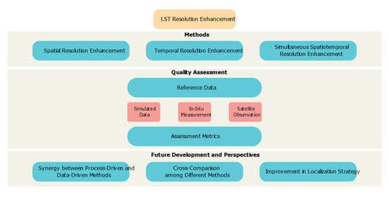
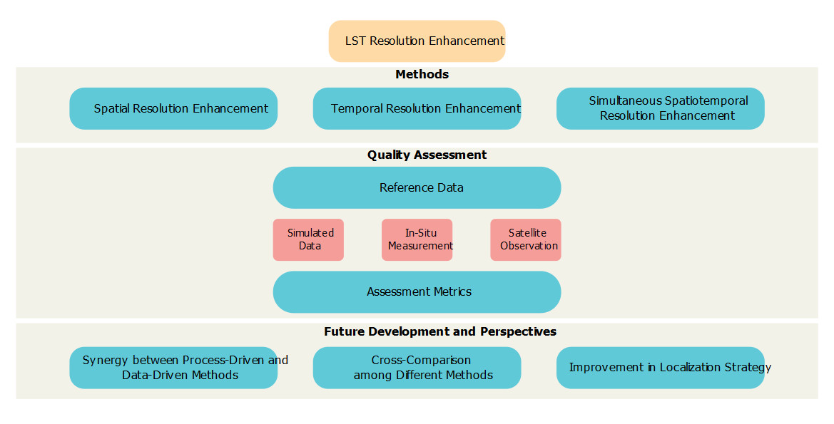
1. Introduction
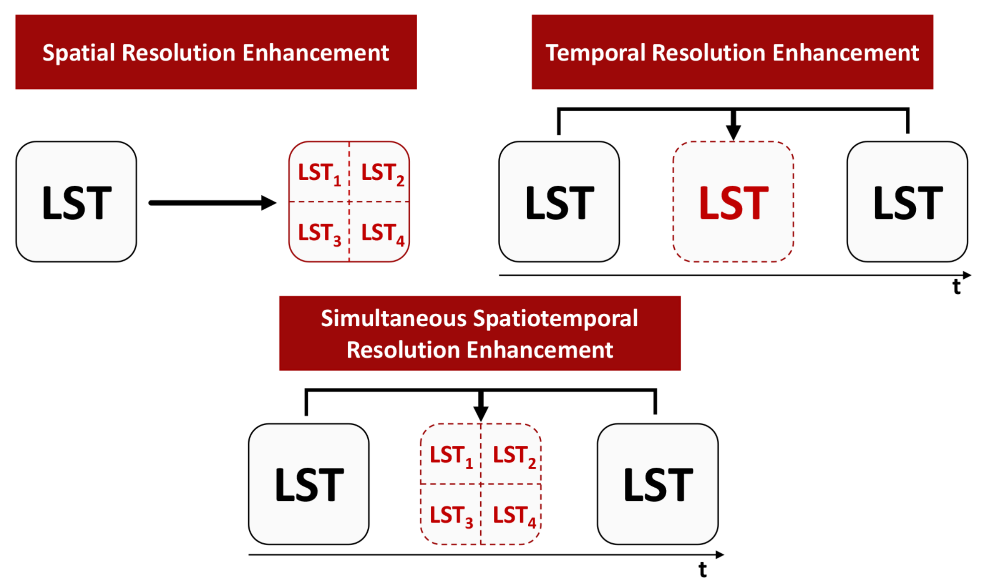
2. Resolution Enhancement Methods
2.1. Spatial Resolution Enhancement
2.1.1. General Process
2.1.2. Regression Kernels and Tools

| Regression Kernel 1 | Category | Literature |
|---|---|---|
| VNIR Reflectance | Image-derived index | [12,33] |
| NDVI | Image-derived index | [8,9,11,13,15,16,18,19,20,25,28,29,32,33,36,38,40,41,42,43,44,45,46,47,48,49,50,51] |
| EVI | Image-derived index | [33,36,52,53,54] |
| NDMI | Image-derived index | [29,36] |
| NMDI | Image-derived index | [55,56] |
| SAVI | Image-derived index | [16,29,33,50,55,56,57,58] |
| NDBI | Image-derived index | [16,19,29,32,33,50,51,55,56,58,59] |
| NDWI | Image-derived index | [33,36,50,55] |
| MNDWI | Image-derived index | [29,33,56] |
| Albedo | Image-derived index | [18,20,43,52,53,60] |
| Emissivity | Image-derived index | [32,33,48,52,53,54,60,61] |
| Fractional vegetation cover | Image-derived index | [9,34,38] |
| DEM | Auxiliary data | [11,12,13,33,51,54,59,60,61] |
| Solar incidence angle | Auxiliary data | [12,33] |
| Land cover classification | Auxiliary data | [12,32,54,61] |
2.1.3. Regression Scale
2.2. Temporal Resolution Enhancement
2.2.1. Interpolation-Based Methods
2.2.2. Fusion-Based Methods
2.3. Simultaneous Spatiotemporal Resolution Enhancement
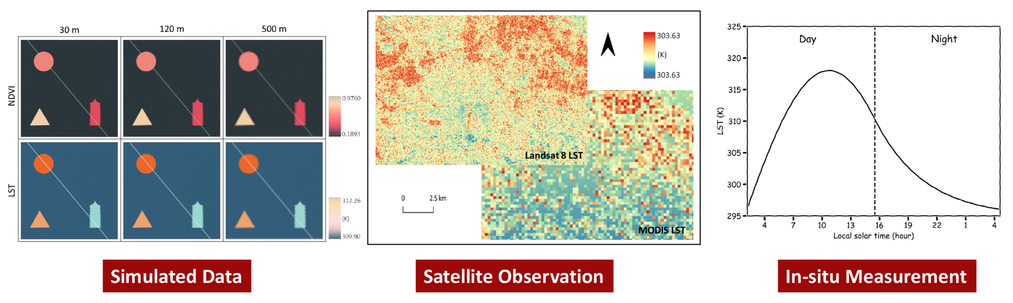
3. Quality Assessment
3.1. Reference Data
3.1.1. Simulated Data
3.1.2. Satellite Observation
3.1.3. In-Situ Measurement
3.2. Assessment Metrics
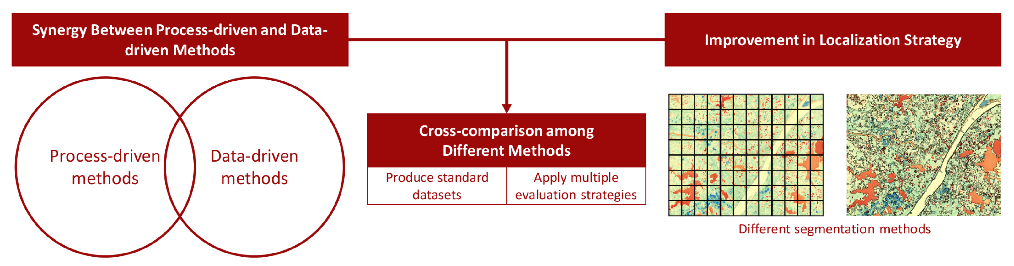
4. Future Development and Perspectives
4.1. Synergy between Process-Driven and Data-Driven Methods
4.2. Cross-Comparison among Different Methods
4.3. Improvement in Localization Strategy
5. Conclusions
Author Contributions
Funding
Data Availability Statement
Conflicts of Interest
References
- Shivers, S.W.; Roberts, D.A.; McFadden, J.P. Using Paired Thermal and Hyperspectral Aerial Imagery to Quantify Land Surface Temperature Variability and Assess Crop Stress within California Orchards. Remote Sens. Environ. 2019, 222, 215–231. [Google Scholar] [CrossRef]
- Chuvieco, E.; Mouillot, F.; van der Werf, G.R.; San Miguel, J.; Tanase, M.; Koutsias, N.; García, M.; Yebra, M.; Padilla, M.; Gitas, I.; et al. Historical Background and Current Developments for Mapping Burned Area from Satellite Earth Observation. Remote Sens. Environ. 2019, 225, 45–64. [Google Scholar] [CrossRef]
- Peng, J.; Qiao, R.; Liu, Y.; Blaschke, T.; Li, S.; Wu, J.; Xu, Z.; Liu, Q. A Wavelet Coherence Approach to Prioritizing Influencing Factors of Land Surface Temperature and Associated Research Scales. Remote Sens. Environ. 2020, 246, 111866. [Google Scholar] [CrossRef]
- Duan, S.B.; Li, Z.L.; Li, H.; Göttsche, F.M.; Wu, H.; Zhao, W.; Leng, P.; Zhang, X.; Coll, C. Validation of Collection 6 MODIS Land Surface Temperature Product Using in Situ Measurements. Remote Sens. Environ. 2019, 225, 16–29. [Google Scholar] [CrossRef]
- Zhu, Z.; Wulder, M.A.; Roy, D.P.; Woodcock, C.E.; Hansen, M.C.; Radeloff, V.C.; Healey, S.P.; Schaaf, C.; Hostert, P.; Strobl, P.; et al. Benefits of the Free and Open Landsat Data Policy. Remote Sens. Environ. 2019, 224, 382–385. [Google Scholar] [CrossRef]
- Campbell, J.B.; Wynne, R.H. Introduction to Remote Sensing, 5th ed.; The Guilford Press: New York, NY, USA, 2011. [Google Scholar]
- Zhu, X.; Cai, F.; Tian, J.; Williams, T. Spatiotemporal Fusion of Multisource Remote Sensing Data: Literature Survey, Taxonomy, Principles, Applications, and Future Directions. Remote Sens. 2018, 10, 527. [Google Scholar] [CrossRef]
- Kustas, W.P.; Norman, J.M.; Anderson, M.C.; French, A.N. Estimating Subpixel Surface Temperatures and Energy Fluxes from the Vegetation Index–Radiometric Temperature Relationship. Remote Sens. Environ. 2003, 85, 429–440. [Google Scholar] [CrossRef]
- Agam, N.; Kustas, W.P.; Anderson, M.C.; Li, F.; Neale, C.M. A Vegetation Index Based Technique for Spatial Sharpening of Thermal Imagery. Remote Sens. Environ. 2007, 107, 545–558. [Google Scholar] [CrossRef]
- Zhan, W.; Chen, Y.; Zhou, J.; Wang, J.; Liu, W.; Voogt, J.; Zhu, X.; Quan, J.; Li, J. Disaggregation of Remotely Sensed Land Surface Temperature: Literature Survey, Taxonomy, Issues, and Caveats. Remote Sens. Environ. 2013, 131, 119–139. [Google Scholar] [CrossRef]
- Duan, S.B.; Li, Z.L. Spatial Downscaling of MODIS Land Surface Temperatures Using Geographically Weighted Regression: Case Study in Northern China. IEEE Trans. Geosci. Remote Sens. 2016, 54, 6458–6469. [Google Scholar] [CrossRef]
- Hutengs, C.; Vohland, M. Downscaling Land Surface Temperatures at Regional Scales with Random Forest Regression. Remote Sens. Environ. 2016, 178, 127–141. [Google Scholar] [CrossRef]
- Bartkowiak, P.; Castelli, M.; Notarnicola, C. Downscaling Land Surface Temperature from MODIS Dataset with Random Forest Approach over Alpine Vegetated Areas. Remote Sens. 2019, 11, 1319. [Google Scholar] [CrossRef]
- Gao, F.; Kustas, W.; Anderson, M. A Data Mining Approach for Sharpening Thermal Satellite Imagery over Land. Remote Sens. 2012, 4, 3287–3319. [Google Scholar] [CrossRef]
- Chen, X.; Li, W.; Chen, J.; Zhan, W.; Rao, Y. A Simple Error Estimation Method for Linear-Regression-Based Thermal Sharpening Techniques with the Consideration of Scale Difference. Geo-Spat. Inf. Sci. 2014, 17, 54–59. [Google Scholar] [CrossRef]
- Xia, H.; Chen, Y.; Quan, J.; Li, J. Object-Based Window Strategy in Thermal Sharpening. Remote Sens. 2019, 11, 634. [Google Scholar] [CrossRef]
- Wu, P.; Shen, H.; Zhang, L.; Göttsche, F.M. Integrated Fusion of Multi-Scale Polar-Orbiting and Geostationary Satellite Observations for the Mapping of High Spatial and Temporal Resolution Land Surface Temperature. Remote Sens. Environ. 2015, 156, 169–181. [Google Scholar] [CrossRef]
- Xia, H.; Chen, Y.; Zhao, Y.; Chen, Z. “Regression-Then-Fusion” or “Fusion-Then-Regression”? A Theoretical Analysis for Generating High Spatiotemporal Resolution Land Surface Temperatures. Remote Sens. 2018, 10, 1382. [Google Scholar] [CrossRef]
- Xia, H.; Chen, Y.; Li, Y.; Quan, J. Combining Kernel-Driven and Fusion-Based Methods to Generate Daily High-Spatial-Resolution Land Surface Temperatures. Remote Sens. Environ. 2019, 224, 259–274. [Google Scholar] [CrossRef]
- Gao, L.; Zhan, W.; Huang, F.; Quan, J.; Lu, X.; Wang, F.; Ju, W.; Zhou, J. Localization or Globalization? Determination of the Optimal Regression Window for Disaggregation of Land Surface Temperature. IEEE Trans. Geosci. Remote Sens. 2017, 55, 477–490. [Google Scholar] [CrossRef]
- Gao, L.; Zhan, W.; Huang, F.; Zhu, X.; Zhou, J.; Quan, J.; Du, P.; Li, M. Disaggregation of Remotely Sensed Land Surface Temperature: A Simple yet Flexible Index (SIFI) to Assess Method Performances. Remote Sens. Environ. 2017, 200, 206–219. [Google Scholar] [CrossRef]
- Quan, J.; Zhan, W.; Ma, T.; Du, Y.; Guo, Z.; Qin, B. An Integrated Model for Generating Hourly Landsat-like Land Surface Temperatures over Heterogeneous Landscapes. Remote Sens. Environ. 2018, 206, 403–423. [Google Scholar] [CrossRef]
- Weng, Q.; Fu, P.; Gao, F. Generating Daily Land Surface Temperature at Landsat Resolution by Fusing Landsat and MODIS Data. Remote Sens. Environ. 2014, 145, 55–67. [Google Scholar] [CrossRef]
- Weng, Q.; Fu, P. Modeling Diurnal Land Temperature Cycles over Los Angeles Using Downscaled GOES Imagery. ISPRS J. Photogramm. Remote Sens. 2014, 97, 78–88. [Google Scholar] [CrossRef]
- Zhan, W.; Chen, Y.; Zhou, J.; Li, J.; Liu, W. Sharpening Thermal Imageries: A Generalized Theoretical Framework From an Assimilation Perspective. IEEE Trans. Geosci. Remote Sens. 2011, 49, 773–789. [Google Scholar] [CrossRef]
- Metz, M.; Andreo, V.; Neteler, M. A New Fully Gap-Free Time Series of Land Surface Temperature from MODIS LST Data. Remote Sens. 2017, 9, 1333. [Google Scholar] [CrossRef]
- Zhu, X.; Helmer, E.H.; Gao, F.; Liu, D.; Chen, J.; Lefsky, M.A. A Flexible Spatiotemporal Method for Fusing Satellite Images with Different Resolutions. Remote Sens. Environ. 2016, 172, 165–177. [Google Scholar] [CrossRef]
- Chen, X.; Li, W.; Chen, J.; Rao, Y.; Yamaguchi, Y. A Combination of TsHARP and Thin Plate Spline Interpolation for Spatial Sharpening of Thermal Imagery. Remote Sens. 2014, 6, 2845–2863. [Google Scholar] [CrossRef]
- Wang, J.W.; Chow, W.T.L.; Wang, Y.C. A Global Regression Method for Thermal Sharpening of Urban Land Surface Temperatures from MODIS and Landsat. Int. J. Remote Sens. 2020, 41, 2986–3009. [Google Scholar] [CrossRef]
- Zhan, W.; Huang, F.; Quan, J.; Zhu, X.; Gao, L.; Zhou, J.; Ju, W. Disaggregation of Remotely Sensed Land Surface Temperature: A New Dynamic Methodology. J. Geophys. Res. Atmos. 2016, 121, 10538–10554. [Google Scholar] [CrossRef]
- Burdun, I.; Bechtold, M.; Sagris, V.; Komisarenko, V.; De Lannoy, G.; Mander, Ü. A Comparison of Three Trapezoid Models Using Optical and Thermal Satellite Imagery for Water Table Depth Monitoring in Estonian Bogs. Remote Sens. 2020, 12, 1980. [Google Scholar] [CrossRef]
- Zawadzka, J.; Corstanje, R.; Harris, J.; Truckell, I. Downscaling Landsat-8 Land Surface Temperature Maps in Diverse Urban Landscapes Using Multivariate Adaptive Regression Splines and Very High Resolution Auxiliary Data. Int. J. Digit. Earth 2020, 13, 899–914. [Google Scholar] [CrossRef]
- Agathangelidis, I.; Cartalis, C. Improving the Disaggregation of MODIS Land Surface Temperatures in an Urban Environment: A Statistical Downscaling Approach Using High-Resolution Emissivity. Int. J. Remote Sens. 2019, 40, 5261–5286. [Google Scholar] [CrossRef]
- Merlin, O.; Duchemin, B.; Hagolle, O.; Jacob, F.; Coudert, B.; Chehbouni, G.; Dedieu, G.; Garatuza, J.; Kerr, Y. Disaggregation of MODIS Surface Temperature over an Agricultural Area Using a Time Series of Formosat-2 Images. Remote Sens. Environ. 2010, 114, 2500–2512. [Google Scholar] [CrossRef]
- Dong, P.; Gao, L.; Zhan, W.; Liu, Z.; Li, J.; Lai, J.; Li, H.; Huang, F.; Tamang, S.K.; Zhao, L. Global Comparison of Diverse Scaling Factors and Regression Models for Downscaling Landsat-8 Thermal Data. ISPRS J. Photogramm. Remote Sens. 2020, 169, 44–56. [Google Scholar] [CrossRef]
- Lillo-Saavedra, M.; García-Pedrero, A.; Merino, G.; Gonzalo-Martín, C. TS2uRF: A New Method for Sharpening Thermal Infrared Satellite Imagery. Remote Sens. 2018, 10, 249. [Google Scholar] [CrossRef]
- Stathopoulou, M.; Cartalis, C. Downscaling AVHRR Land Surface Temperatures for Improved Surface Urban Heat Island Intensity Estimation. Remote Sens. Environ. 2009, 113, 2592–2605. [Google Scholar] [CrossRef]
- Amazirh, A.; Merlin, O.; Er-Raki, S. Including Sentinel-1 Radar Data to Improve the Disaggregation of MODIS Land Surface Temperature Data. ISPRS J. Photogramm. Remote Sens. 2019, 150, 11–26. [Google Scholar] [CrossRef]
- Maeda, E.E. Downscaling MODIS LST in the East African Mountains Using Elevation Gradient and Land-Cover Information. Int. J. Remote Sens. 2014, 35, 3094–3108. [Google Scholar] [CrossRef]
- Zhang, X.; Zhao, H.; Yang, J. Spatial Downscaling of Land Surface Temperature in Combination with TVDI and Elevation. Int. J. Remote Sens. 2019, 40, 1875–1886. [Google Scholar] [CrossRef]
- Liu, K.; Wang, S.; Li, X.; Li, Y.; Zhang, B.; Zhai, R. The Assessment of Different Vegetation Indices for Spatial Disaggregating of Thermal Imagery over the Humid Agricultural Region. Int. J. Remote Sens. 2020, 41, 1907–1926. [Google Scholar] [CrossRef]
- Zhou, J.; Liu, S.; Li, M.; Zhan, W.; Xu, Z.; Xu, T. Quantification of the Scale Effect in Downscaling Remotely Sensed Land Surface Temperature. Remote Sens. 2016, 8, 975. [Google Scholar] [CrossRef]
- Dominguez, A.; Kleissl, J.; Luvall, J.C.; Rickman, D.L. High-Resolution Urban Thermal Sharpener (HUTS). Remote Sens. Environ. 2011, 115, 1772–1780. [Google Scholar] [CrossRef]
- Inamdar, A.K.; French, A.; Hook, S.; Vaughan, G.; Luckett, W. Land Surface Temperature Retrieval at High Spatial and Temporal Resolutions over the Southwestern United States. J. Geophys. Res. Atmos. 2008, 113. [Google Scholar] [CrossRef]
- Bechtel, B.; Zakšek, K.; Hoshyaripour, G. Downscaling Land Surface Temperature in an Urban Area: A Case Study for Hamburg, Germany. Remote Sens. 2012, 4, 3184–3200. [Google Scholar] [CrossRef]
- Chen, X.; Yamaguchi, Y.; Chen, J.; Shi, Y. Scale Effect of Vegetation-Index-Based Spatial Sharpening for Thermal Imagery: A Simulation Study by ASTER Data. IEEE Geosci. Remote Sens. Lett. 2012, 9, 549–553. [Google Scholar] [CrossRef]
- Bindhu, V.; Narasimhan, B.; Sudheer, K. Development and Verification of a Non-Linear Disaggregation Method (NL-DisTrad) to Downscale MODIS Land Surface Temperature to the Spatial Scale of Landsat Thermal Data to Estimate Evapotranspiration. Remote Sens. Environ. 2013, 135, 118–129. [Google Scholar] [CrossRef]
- Ghosh, A.; Joshi, P.K. Hyperspectral Imagery for Disaggregation of Land Surface Temperature with Selected Regression Algorithms over Different Land Use Land Cover Scenes. ISPRS J. Photogramm. Remote Sens. 2014, 96, 76–93. [Google Scholar] [CrossRef]
- Cho, K.; Kim, Y.; Kim, Y. Disaggregation of Landsat-8 Thermal Data Using Guided SWIR Imagery on the Scene of a Wildfire. Remote Sens. 2018, 10, 105. [Google Scholar] [CrossRef]
- Pan, X.; Zhu, X.; Yang, Y.; Cao, C.; Zhang, X.; Shan, L. Applicability of Downscaling Land Surface Temperature by Using Normalized Difference Sand Index. Sci. Rep. 2018, 8, 9530. [Google Scholar] [CrossRef]
- Wang, R.; Gao, W.; Peng, W. Downscale MODIS Land Surface Temperature Based on Three Different Models to Analyze Surface Urban Heat Island: A Case Study of Hangzhou. Remote Sens. 2020, 12, 2134. [Google Scholar] [CrossRef]
- Zakšek, K.; Oštir, K. Downscaling Land Surface Temperature for Urban Heat Island Diurnal Cycle Analysis. Remote Sens. Environ. 2012, 117, 114–124. [Google Scholar] [CrossRef]
- Jiang, Y.; Fu, P.; Weng, Q. Downscaling GOES Land Surface Temperature for Assessing Heat Wave Health Risks. IEEE Geosci. Remote Sens. Lett. 2015, 12, 1605–1609. [Google Scholar] [CrossRef]
- Sismanidis, P.; Keramitsoglou, I.; Kiranoudis, C.T.; Bechtel, B. Assessing the Capability of a Downscaled Urban Land Surface Temperature Time Series to Reproduce the Spatiotemporal Features of the Original Data. Remote Sens. 2016, 8, 274. [Google Scholar] [CrossRef]
- Yang, G.; Pu, R.; Zhao, C.; Huang, W.; Wang, J. Estimation of Subpixel Land Surface Temperature Using an Endmember Index Based Technique: A Case Examination on ASTER and MODIS Temperature Products over a Heterogeneous Area. Remote Sens. Environ. 2011, 115, 1202–1219. [Google Scholar] [CrossRef]
- Yang, Y.; Cao, C.; Pan, X.; Li, X.; Zhu, X. Downscaling Land Surface Temperature in an Arid Area by Using Multiple Remote Sensing Indices with Random Forest Regression. Remote Sens. 2017, 9, 789. [Google Scholar] [CrossRef]
- Yang, G.; Pu, R.; Huang, W.; Wang, J.; Zhao, C. A Novel Method to Estimate Subpixel Temperature by Fusing Solar-Reflective and Thermal-Infrared Remote-Sensing Data With an Artificial Neural Network. IEEE Trans. Geosci. Remote Sens. 2010, 48, 2170–2178. [Google Scholar] [CrossRef]
- Bonafoni, S. Downscaling of Landsat and MODIS Land Surface Temperature Over the Heterogeneous Urban Area of Milan. IEEE J. Sel. Top. Appl. Earth Obs. Remote Sens. 2016, 9, 2019–2027. [Google Scholar] [CrossRef]
- Peng, Y.; Li, W.; Luo, X.; Li, H. A Geographically and Temporally Weighted Regression Model for Spatial Downscaling of MODIS Land Surface Temperatures Over Urban Heterogeneous Regions. IEEE Trans. Geosci. Remote Sens. 2019, 57, 5012–5027. [Google Scholar] [CrossRef]
- Sismanidis, P.; Keramitsoglou, I.; Bechtel, B.; Kiranoudis, C.T. Improving the Downscaling of Diurnal Land Surface Temperatures Using the Annual Cycle Parameters as Disaggregation Kernels. Remote Sens. 2017, 9, 23. [Google Scholar] [CrossRef]
- Keramitsoglou, I.; Kiranoudis, C.T.; Weng, Q. Downscaling Geostationary Land Surface Temperature Imagery for Urban Analysis. IEEE Geosci. Remote Sens. Lett. 2013, 10, 1253–1257. [Google Scholar] [CrossRef]
- Jeganathan, C.; Hamm, N.; Mukherjee, S.; Atkinson, P.; Raju, P.; Dadhwal, V. Evaluating a Thermal Image Sharpening Model over a Mixed Agricultural Landscape in India. Int. J. Appl. Earth Obs. Geoinf. 2011, 13, 178–191. [Google Scholar] [CrossRef]
- Li, W.; Ni, L.; Li, Z.; Duan, S.; Wu, H. Evaluation of Machine Learning Algorithms in Spatial Downscaling of MODIS Land Surface Temperature. IEEE J. Sel. Top. Appl. Earth Obs. Remote Sens. 2019, 12, 2299–2307. [Google Scholar] [CrossRef]
- Kolios, S.; Georgoulas, G.; Stylios, C. Achieving Downscaling of Meteosat Thermal Infrared Imagery Using Artificial Neural Networks. Int. J. Remote Sens. 2013, 34, 7706–7722. [Google Scholar] [CrossRef]
- Ebrahimy, H.; Azadbakht, M. Downscaling MODIS Land Surface Temperature over a Heterogeneous Area: An Investigation of Machine Learning Techniques, Feature Selection, and Impacts of Mixed Pixels. Comput. Geosci. 2019, 124, 93–102. [Google Scholar] [CrossRef]
- Wu, H.; Li, W. Downscaling Land Surface Temperatures Using a Random Forest Regression Model With Multitype Predictor Variables. IEEE Access 2019, 7, 21904–21916. [Google Scholar] [CrossRef]
- Zhu, X.; Tuia, D.; Mou, L.; Xia, G.; Zhang, L.; Xu, F.; Fraundorfer, F. Deep Learning in Remote Sensing: A Comprehensive Review and List of Resources. IEEE Geosci. Remote Sens. Mag. 2017, 5, 8–36. [Google Scholar] [CrossRef]
- Ma, L.; Liu, Y.; Zhang, X.; Ye, Y.; Yin, G.; Johnson, B.A. Deep Learning in Remote Sensing Applications: A Meta-Analysis and Review. ISPRS J. Photogramm. Remote Sens. 2019, 152, 166–177. [Google Scholar] [CrossRef]
- Marceau, D.J.; Hay, G.J. Remote Sensing Contributions to the Scale Issue. Can. J. Remote Sens. 1999, 25, 357–366. [Google Scholar] [CrossRef]
- Mukherjee, S.; Joshi, P.K.; Garg, R.D. A Comparison of Different Regression Models for Downscaling Landsat and MODIS Land Surface Temperature Images over Heterogeneous Landscape. Adv. Space Res. 2014, 54, 655–669. [Google Scholar] [CrossRef]
- Zhukov, B.; Oertel, D.; Lanzl, F.; Reinhackel, G. Unmixing-Based Multisensor Multiresolution Image Fusion. IEEE Trans. Geosci. Remote Sens. 1999, 37, 1212–1226. [Google Scholar] [CrossRef]
- Zhan, W.; Chen, Y.; Wang, J.; Zhou, J.; Quan, J.; Liu, W.; Li, J. Downscaling Land Surface Temperatures with Multi-Spectral and Multi-Resolution Images. Int. J. Appl. Earth Obs. Geoinf. 2012, 18, 23–36. [Google Scholar] [CrossRef]
- Göttsche, F.M.; Olesen, F.S. Modelling the Effect of Optical Thickness on Diurnal Cycles of Land Surface Temperature. Remote Sens. Environ. 2009, 113, 2306–2316. [Google Scholar] [CrossRef]
- Zhu, X.; Chen, J.; Gao, F.; Chen, X.; Masek, J.G. An Enhanced Spatial and Temporal Adaptive Reflectance Fusion Model for Complex Heterogeneous Regions. Remote Sens. Environ. 2010, 114, 2610–2623. [Google Scholar] [CrossRef]
- Göttsche, F.M.; Olesen, F.S. Modelling of Diurnal Cycles of Brightness Temperature Extracted from METEOSAT Data. Remote Sens. Environ. 2001, 76, 337–348. [Google Scholar] [CrossRef]
- Huang, F.; Zhan, W.; Duan, S.B.; Ju, W.; Quan, J. A Generic Framework for Modeling Diurnal Land Surface Temperatures with Remotely Sensed Thermal Observations under Clear Sky. Remote Sens. Environ. 2014, 150, 140–151. [Google Scholar] [CrossRef]
- Liu, X.; Tang, B.H.; Li, Z.L.; Zhou, C.; Wu, W.; Rasmussen, M.O. An Improved Method for Separating Soil and Vegetation Component Temperatures Based on Diurnal Temperature Cycle Model and Spatial Correlation. Remote Sens. Environ. 2020, 248, 111979. [Google Scholar] [CrossRef]
- Duan, S.B.; Li, Z.L.; Wang, N.; Wu, H.; Tang, B.H. Evaluation of Six Land-Surface Diurnal Temperature Cycle Models Using Clear-Sky in Situ and Satellite Data. Remote Sens. Environ. 2012, 124, 15–25. [Google Scholar] [CrossRef]
- Jin, M.; Dickinson, R.E. Interpolation of Surface Radiative Temperature Measured from Polar Orbiting Satellites to a Diurnal Cycle: 1. Without Clouds. J. Geophys. Res. Atmos. 1999, 104, 2105–2116. [Google Scholar] [CrossRef]
- Sun, D.; Pinker, R.T. Implementation of GOES-based Land Surface Temperature Diurnal Cycle to AVHRR. Int. J. Remote Sens. 2005, 26, 3975–3984. [Google Scholar] [CrossRef]
- Duan, S.B.; Li, Z.L.; Wu, H.; Tang, B.H.; Jiang, X.; Zhou, G. Modeling of Day-to-Day Temporal Progression of Clear-Sky Land Surface Temperature. IEEE Geosci. Remote Sens. Lett. 2013, 10, 1050–1054. [Google Scholar] [CrossRef]
- Weng, Q.; Fu, P. Modeling Annual Parameters of Clear-Sky Land Surface Temperature Variations and Evaluating the Impact of Cloud Cover Using Time Series of Landsat TIR Data. Remote Sens. Environ. 2014, 140, 267–278. [Google Scholar] [CrossRef]
- Zhan, W.; Zhou, J.; Ju, W.; Li, M.; Sandholt, I.; Voogt, J.; Yu, C. Remotely Sensed Soil Temperatures beneath Snow-Free Skin-Surface Using Thermal Observations from Tandem Polar-Orbiting Satellites: An Analytical Three-Time-Scale Model. Remote Sens. Environ. 2014, 143, 1–14. [Google Scholar] [CrossRef]
- Stine, A.R.; Huybers, P.; Fung, I.Y. Changes in the Phase of the Annual Cycle of Surface Temperature. Nature 2009, 457, 435–440. [Google Scholar] [CrossRef] [PubMed]
- Quan, J.; Chen, Y.; Zhan, W.; Wang, J.; Voogt, J.; Li, J. A Hybrid Method Combining Neighborhood Information from Satellite Data with Modeled Diurnal Temperature Cycles over Consecutive Days. Remote Sens. Environ. 2014, 155, 257–274. [Google Scholar] [CrossRef]
- Thomas, C.; Ranchin, T.; Wald, L.; Chanussot, J. Synthesis of Multispectral Images to High Spatial Resolution: A Critical Review of Fusion Methods Based on Remote Sensing Physics. IEEE Trans. Geosci. Remote Sens. 2008, 46, 1301–1312. [Google Scholar] [CrossRef]
- Schmitt, M.; Zhu, X.X. Data Fusion and Remote Sensing: An Ever-Growing Relationship. IEEE Geosci. Remote Sens. Mag. 2016, 4, 6–23. [Google Scholar] [CrossRef]
- Pohl, C.; van Genderen, J. Remote Sensing Image Fusion: An Update in the Context of Digital Earth. Int. J. Digit. Earth 2014, 7, 158–172. [Google Scholar] [CrossRef]
- Belgiu, M.; Stein, A. Spatiotemporal Image Fusion in Remote Sensing. Remote Sens. 2019, 11, 818. [Google Scholar] [CrossRef]
- Liu, H.; Weng, Q. Enhancing Temporal Resolution of Satellite Imagery for Public Health Studies: A Case Study of West Nile Virus Outbreak in Los Angeles in 2007. Remote Sens. Environ. 2012, 117, 57–71. [Google Scholar] [CrossRef]
- Gao, F.; Masek, J.; Schwaller, M.; Hall, F. On the Blending of the Landsat and MODIS Surface Reflectance: Predicting Daily Landsat Surface Reflectance. IEEE Trans. Geosci. Remote Sens. 2006, 44, 2207–2218. [Google Scholar] [CrossRef]
- Wu, M.; Niu, Z.; Wang, C.; Wu, C.; Wang, L. Use of MODIS and Landsat Time Series Data to Generate High-Resolution Temporal Synthetic Landsat Data Using a Spatial and Temporal Reflectance Fusion Model. J. Appl. Remote Sens. 2012, 6, 063507. [Google Scholar] [CrossRef]
- Wu, M.; Li, H.; Huang, W.; Niu, Z.; Wang, C. Generating Daily High Spatial Land Surface Temperatures by Combining ASTER and MODIS Land Surface Temperature Products for Environmental Process Monitoring. Environ. Sci. Process. Impacts 2015, 17, 1396–1404. [Google Scholar] [CrossRef] [PubMed]
- Wu, P.; Shen, H.; Ai, T.; Liu, Y. Land-Surface Temperature Retrieval at High Spatial and Temporal Resolutions Based on Multi-Sensor Fusion. Int. J. Digit. Earth 2013, 6, 113–133. [Google Scholar] [CrossRef]
- Moosavi, V.; Talebi, A.; Mokhtari, M.H.; Shamsi, S.R.F.; Niazi, Y. A Wavelet-Artificial Intelligence Fusion Approach (WAIFA) for Blending Landsat and MODIS Surface Temperature. Remote Sens. Environ. 2015, 169, 243–254. [Google Scholar] [CrossRef]
- Shao, Z.; Cai, J.; Fu, P.; Hu, L.; Liu, T. Deep Learning-Based Fusion of Landsat-8 and Sentinel-2 Images for a Harmonized Surface Reflectance Product. Remote Sens. Environ. 2019, 235, 111425. [Google Scholar] [CrossRef]
- Bai, Y.; Wong, M.; Shi, W.Z.; Wu, L.X.; Qin, K. Advancing of Land Surface Temperature Retrieval Using Extreme Learning Machine and Spatio-Temporal Adaptive Data Fusion Algorithm. Remote Sens. 2015, 7, 4424–4441. [Google Scholar] [CrossRef]
- Zhou, J.; Chen, Y.; Zhang, X.; Zhan, W. Modelling the Diurnal Variations of Urban Heat Islands with Multi-Source Satellite Data. Int. J. Remote Sens. 2013, 34, 7568–7588. [Google Scholar] [CrossRef]
- Wang, W.; Liang, S.; Meyers, T. Validating MODIS Land Surface Temperature Products Using Long-Term Nighttime Ground Measurements. Remote Sens. Environ. 2008, 112, 623–635. [Google Scholar] [CrossRef]
- Zurita-Milla, R.; Kaiser, G.; Clevers, J.G.P.W.; Schneider, W.; Schaepman, M.E. Downscaling Time Series of MERIS Full Resolution Data to Monitor Vegetation Seasonal Dynamics. Remote Sens. Environ. 2009, 113, 1874–1885. [Google Scholar] [CrossRef]
- Rodriguez-Galiano, V.; Pardo-Iguzquiza, E.; Sanchez-Castillo, M.; Chica-Olmo, M.; Chica-Rivas, M. Downscaling Landsat 7 ETM+ Thermal Imagery Using Land Surface Temperature and NDVI Images. Int. J. Appl. Earth Obs. Geoinf. 2012, 18, 515–527. [Google Scholar] [CrossRef]
- Wang, Z.; Bovik, A.C.; Sheikh, H.R.; Simoncelli, E.P. Image Quality Assessment: From Error Visibility to Structural Similarity. IEEE Trans. Image Process. 2004, 13, 600–612. [Google Scholar] [CrossRef] [PubMed]
- Wang, Z.; Bovik, A.C. A Universal Image Quality Index. IEEE Signal Process. Lett. 2002, 9, 81–84. [Google Scholar] [CrossRef]
- Reichstein, M.; Camps-Valls, G.; Stevens, B.; Jung, M.; Denzler, J.; Carvalhais, N.; Prabhat. Deep Learning and Process Understanding for Data-Driven Earth System Science. Nature 2019, 566, 195–204. [Google Scholar] [CrossRef]
- Steffen, W.; Richardson, K.; Rockström, J.; Schellnhuber, H.J.; Dube, O.P.; Dutreuil, S.; Lenton, T.M.; Lubchenco, J. The Emergence and Evolution of Earth System Science. Nat. Rev. Earth Environ. 2020, 1, 54–63. [Google Scholar] [CrossRef]
- Belgiu, M.; Drăguţ, L. Random Forest in Remote Sensing: A Review of Applications and Future Directions. ISPRS J. Photogramm. Remote Sens. 2016, 114, 24–31. [Google Scholar] [CrossRef]
- Audebert, N.; Saux, B.L.; Lefevre, S. Deep Learning for Classification of Hyperspectral Data: A Comparative Review. IEEE Geosci. Remote Sens. Mag. 2019, 7, 159–173. [Google Scholar] [CrossRef]
- Vali, A.; Comai, S.; Matteucci, M. Deep Learning for Land Use and Land Cover Classification Based on Hyperspectral and Multispectral Earth Observation Data: A Review. Remote Sens. 2020, 12, 2495. [Google Scholar] [CrossRef]
- Murphy, J.M.; Maggioni, M. Unsupervised Clustering and Active Learning of Hyperspectral Images With Nonlinear Diffusion. IEEE Trans. Geosci. Remote Sens. 2019, 57, 1829–1845. [Google Scholar] [CrossRef]
- Gorelick, N.; Hancher, M.; Dixon, M.; Ilyushchenko, S.; Thau, D.; Moore, R. Google Earth Engine: Planetary-Scale Geospatial Analysis for Everyone. Remote Sens. Environ. 2017, 202, 18–27. [Google Scholar] [CrossRef]


| Sensor | Satellite | Spectral Ranges of TIR Bands (µm) | Spatial Resolution | Observation Frequency | Operational Period | Data Access1 |
|---|---|---|---|---|---|---|
| AVHRR | NOAA | 10.5–11.3; 11.5–12.5 | 1.1 km | Twice daily | Since 1979 | https://earthexplorer.usgs.gov/ |
| TM | Landsat 4 | 10.4–12.5 | 120 m | 16 days | From 1982 to 1993 | https://landsatlook.usgs.gov/ |
| TM | Landsat 5 | 10.4–12.5 | 120 m | 16 days | From 1984 to 2013 | https://landsatlook.usgs.gov/ |
| ETM+ | Landsat 7 | 10.4–12.5 | 60 m | 16 days | Since 1999 | https://landsatlook.usgs.gov/ |
| TIRS | Landsat 8 | 10.60–11.19; 11.50–12.51 | 100 m | 16 days | Since 2013 | https://landsatlook.usgs.gov/ |
| MODIS | Terra/Aqua | 10.78–11.28; 11.77–12.27 | 1 km | Twice daily | Since 1999/2002 | https://modis.gsfc.nasa.gov/ |
| ASTER | Terra | 8.125–8.475; 8.475–8.825; 8.925–9.275; 10.25–10.95; 10.95–11.65 | 90 m | 16 days | Since 1999 | https://earthexplorer.usgs.gov/ |
| AATSR | Envisat | 11; 12 (center) | 1 km | 35 days | Since 2002 | https://earth.esa.int/ |
| SLSTR | Sentinel-3 (A/B) | 10.85; 12.02 (center) | 1 km | 1 day | Since 2016/2018 | https://sentinel.esa.int/ |
| VIRR | Fengyun-3 (B/C) | 10.3–11.3; 11.5–12.5 | 1.1 km | Twice daily | Since 2010/2013 | http://satellite.nsmc.org.cn/ |
| IRMSS | HJ-1B | 10.5–12.5 | 300 m | 31 days | Since 2008 | www.chinageoss.cn |
| GOES Imager | GOES | 10.2–11.2; 11.5–12.5 | 4 km | 3 h (Geostationary) | Since 1975 | https://www.star.nesdis.noaa.gov/GOES/index.php |
| SEVIRI | MSG | 9.8–11.8; 11.0–13.0 | 3 km | 15 min (Geostationary) | Since 2005 | https://landsaf.ipma.pt/ |
| AGRI | Fengyun-4A | 8.0–9.0; 10.3–11.3; 11.5–12.5; 13.2–13.8 | 4 km | 36 min (Geostationary) | Since 2016 | http://satellite.nsmc.org.cn/ |
Publisher’s Note: MDPI stays neutral with regard to jurisdictional claims in published maps and institutional affiliations. |
© 2021 by the authors. Licensee MDPI, Basel, Switzerland. This article is an open access article distributed under the terms and conditions of the Creative Commons Attribution (CC BY) license (http://creativecommons.org/licenses/by/4.0/).
Share and Cite
Mao, Q.; Peng, J.; Wang, Y. Resolution Enhancement of Remotely Sensed Land Surface Temperature: Current Status and Perspectives. Remote Sens. 2021, 13, 1306. https://doi.org/10.3390/rs13071306
Mao Q, Peng J, Wang Y. Resolution Enhancement of Remotely Sensed Land Surface Temperature: Current Status and Perspectives. Remote Sensing. 2021; 13(7):1306. https://doi.org/10.3390/rs13071306
Chicago/Turabian StyleMao, Qi, Jian Peng, and Yanglin Wang. 2021. "Resolution Enhancement of Remotely Sensed Land Surface Temperature: Current Status and Perspectives" Remote Sensing 13, no. 7: 1306. https://doi.org/10.3390/rs13071306
APA StyleMao, Q., Peng, J., & Wang, Y. (2021). Resolution Enhancement of Remotely Sensed Land Surface Temperature: Current Status and Perspectives. Remote Sensing, 13(7), 1306. https://doi.org/10.3390/rs13071306