Article

Automated Mapping of Transportation Embankments in Fine-Resolution LiDAR DEMs

Department of Geography, Environment & Geomatics, The University of Guelph, 50 Stone Rd. E, Guelph, ON N1G 2W1, Canada
*
Author to whom correspondence should be addressed.
Remote Sens. 2021, 13(7), 1308; https://doi.org/10.3390/rs13071308
Submission received: 26 February 2021 / Revised: 24 March 2021 / Accepted: 29 March 2021 / Published: 30 March 2021
(This article belongs to the Special Issue Perspectives on Digital Elevation Model Applications)

Abstract

:
Fine-resolution LiDAR DEMs can represent surface features such as road and railway embankments with high fidelity. However, transportation embankments are problematic for several environmental modelling applications, and particularly hydrological modelling. Currently, there are no automated techniques for the identification and removal of embankments from LiDAR DEMs. This paper presents a novel algorithm for identifying embankments in LiDAR DEMs. The algorithm utilizes repositioned transportation network cells as seed points in a region-growing operation. The embankment region grows based on derived morphometric parameters, including road surface width, embankment width, embankment height, and absolute slope. The technique was tested on eight LiDAR DEMs representing subsections of four watersheds in southwestern Ontario, Canada, ranging in size from 16 million cells to 134 million cells. The algorithm achieved a recall greater than or equal to 90% for seven of the eight DEMs, while achieving a Pearson’s phi correlation coefficient greater than 80% for five of the eight DEMs. Therefore, the method has moderate to high accuracy for identifying embankments. The processing times associated with applying the technique to the eight study site DEMs ranged from 1.4 s to 20.3 s, which demonstrates the practicality of using the embankment mapping tool in applications with data set sizes commonly encountered in practice.

1. Introduction

Fine-resolution digital elevation models (DEMs) such as those derived from light detection and ranging (LiDAR) are valuable for environmental modelling because these DEMs can represent topographic detail with high fidelity [1]. One consequence of this detail is the representation of surface features such as transportation embankments. In agricultural and rural areas, road and railway embankments are constructed to maintain a stable gradient across a landscape and to reduce the impact of flooding on transportation infrastructure by elevating roads and railways above the surrounding terrain [2,3]. These transportation embankments often have parallel ditches and embedded culverts to facilitate drainage off of, and away from, the embankment. This stands in contrast to roads and railways in urban settings, which are typically level with the ground surface and drained by sub-surface sewers.
Although the embankment surface and associated ditches are faithfully captured in fine-resolution DEMs, the culverts that pass beneath embankments are not [1,4,5]. Without culverts, digital embankments become artefact dams that exhibit different hydrological behaviour than real embankments. Digital embankments can create extensive upslope areas of artefact depressions, which impede the modelling of hydrological flow and connectivity, and influence modelled flood potential and contaminant delivery [1,4,6,7,8,9,10]. Typically, it is best to employ hydrological conditioning techniques such as filling and breaching to remove artefact depressions created by embankments [1,4,11,12]. However, these conditioning techniques cannot recreate a pre-embankment surface necessary for applications such as historical flow modelling.
Furthermore, the topographic influence of embankments extends into the areas adjacent to embankments and interferes with the derivation of terrain attributes based on local neighbourhoods, such as slope, which are often required for applications such as predictive soil mapping, vegetation distribution mapping, and wetland mapping [13,14,15,16]. For such applications, hydrological conditioning techniques do not eliminate the local topographic effects of embankments.
Therefore, for some modelling applications, there is a need to identify and remove embankments in their entirety to improve the accuracy of environmental models impacted by embankments. Currently, there are no automated techniques to identify or remove embankments. This paper presents a novel region-growing algorithm for mapping transportation embankments in fine-resolution LiDAR DEMs. This method is raster-based rather than point-cloud based because of the complexities of processing point cloud data and the greater availability of raster DEM data, thus making the algorithm widely applicable to practitioners.
Roads and railways, and thus the embankments they are constructed on, are largely linear features. There are many techniques traditionally used in remote sensing for mapping radiometrically uniform linear features in imagery data, including edge and line detection, the Hough and wavelet transforms, and mathematical morphological approaches [17,18,19,20,21,22]. However, DEMs are surfaces, not images, and features such as embankments in DEMs are not uniform in elevation or first or second order derivatives. Thus, the aforementioned techniques were deemed inappropriate for the development of an embankment mapping algorithm. Instead, a region growing approach was chosen because existing transportation network vectors offered high-quality seed points for classifying embankments in DEMs.

2. Materials and Methods

2.1. Embankment Mapping Algorithm

The following sections describe each of the components of the embankment mapping algorithm used by the tool. The algorithm begins by selecting and repositioning seed points. Parameters are then derived to serve as growth conditions for the region growing component of the algorithm (Table 1). Finally, the embankment region is grown from the seed points using the derived parameters.

2.1.1. Seed Selection

Region growing is a segmentation technique that can be used to identify distinct features in rasters, such as DEMs [17,23]. The first step in a region-growing operation is the selection of starting cells, sometimes called seed points. The mapped region then grows outwards from each of the initialization seeds, classifying neighbouring cells as part of the region if those cells are within a pre-defined similarity threshold, or set of thresholds, based on a set of conditional criteria [17,23].
The road embankment mapping algorithm described in this paper utilizes the cells of a rasterized transportation network (derived from mapped road and railway line vectors) as seed points. Transportation network cells should be found atop transportation embankments, usually in a medial position, and thus these cells serve as ideal starting points for embankment mapping. However, depending on data quality, some transportation vectors can be misaligned with embankments, positioned either to the side of the embankment or off the embankment entirely. This situation can result in poor classification of embankments and unwanted classification of non-embankment cells. To solve the vector alignment problem, the embankment mapping algorithm begins by repositioning seed cells to the highest, non-seed location within their local neighbourhoods, the size of which is provided by the seed repositioning search distance parameter. Under most circumstances, the center of the nearest embankment should represent the highest elevation within the search distance.

2.1.2. Parameter Derivation

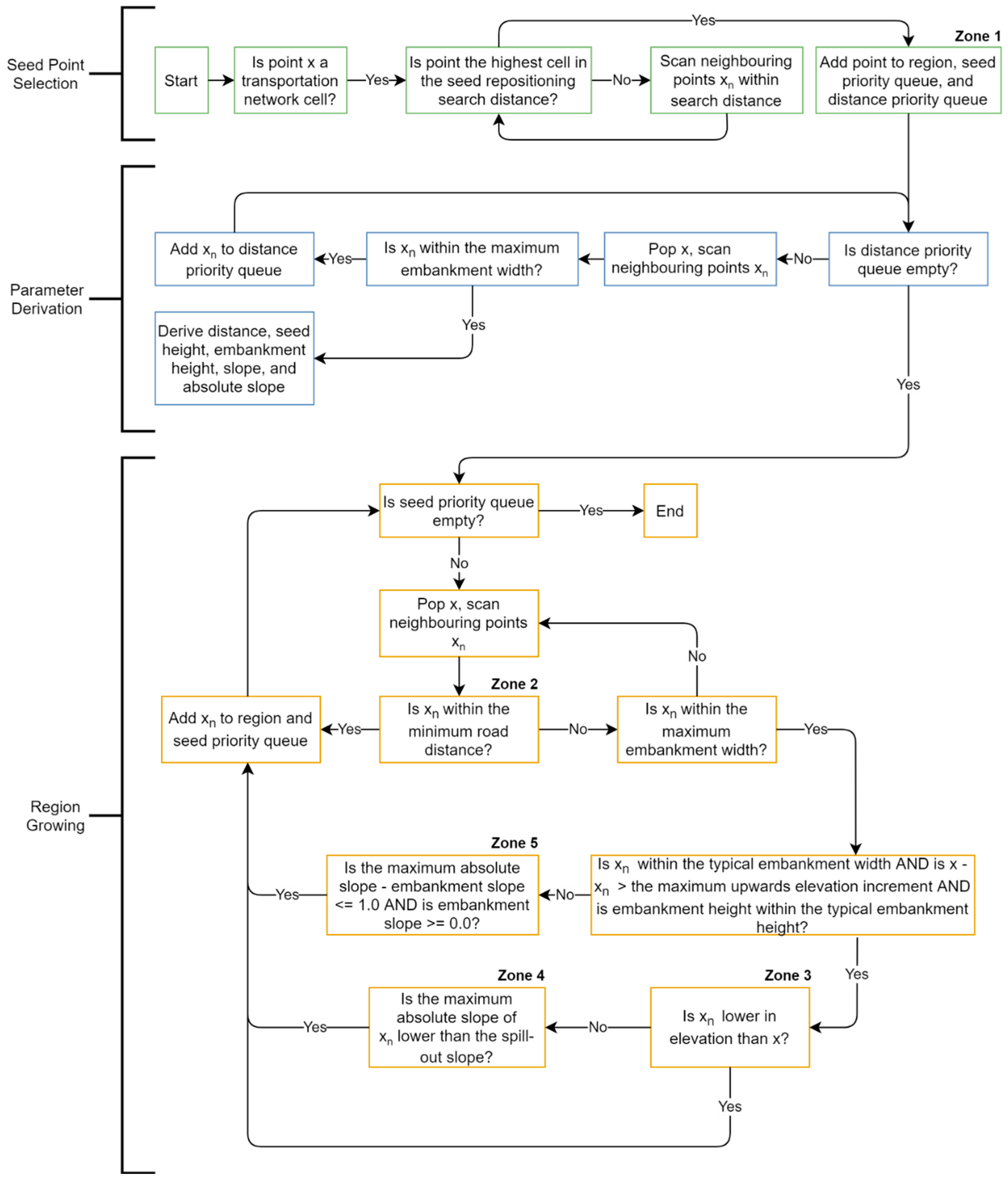
Once a seed cell has been repositioned, it is added to the classified embankment region, a seed priority queue (SPQ), and a distance priority queue (DPQ). A priority queue is a list of values that follows a first-in-first-out (FIFO) principle where values are dequeued (i.e., popped) based on a priority value [24]. For both the SPQ and the DPQ, grid cells are dequeued based on their distance to the nearest seed cell, such that cells closer to seed cells are dealt with before those further from seeds. The seed priority queue is used to store seed points for the region growing algorithm. The distance priority queue is used to store each cell within the maximum embankment width so that morphometric parameters can be derived for those cells.
Before the embankment region is grown, the morphometric parameters used to map embankments must be derived using the DPQ. Each cell, x, is popped from the DPQ and each of the eight neighbours, xn, is scanned. If xn is within the maximum embankment width relative to the repositioned seed cells, xn is added to the DPQ and parameters for xn are derived. These parameters include (1) the distance of xn to the nearest seed cell, (2) the elevation difference between a cell and its nearest seed cell (i.e., the height of the embankment at xn), (3) the slope of the embankment at xn, and (4) the maximum absolute slope at xn, defined as the largest slope encountered between xn and its nearest seed cell. This process continues until every cell in the DPQ has been scanned and the morphometric parameters for embankments have been derived.

2.1.3. Region Growing

Figure 1 presents a model of a ditch-lined embankment (Figure 1A) and a model of an embankment at a valley crossing (Figure 1B), which are used to illustrate several embankment zones identified in the region-growing algorithm for embankment mapping.
Zone 1 corresponds to the transportation network seed cells, which because of the typical construction of road surfaces, should be situated along the embankment medial line. Zone 2 represents the surface of the embankment, which corresponds to the width of the level road/rail embankment top. Zones 3 and 4 correspond to the sides and ditches of a ditch-lined embankment, and the distinction between these two zones is explained further below. Zone 5 corresponds to the relatively steep sides of an embankment in places where the embankment traverses a valley or other low point in the landscape.
Each grid cell x is popped from the SPQ and each neighbour xn is scanned. If the distance between x and xn is less than half of the minimum road width, xn falls within Zone 2 and is added to the SPQ and classified as part of the embankment region. Within Zone 2, the growth of the region is constrained only by the distance to the nearest seed; changes in elevation or slope are inconsequential on the road or railway surface. This condition ensures satisfactory classification of the road or railway surface.
Beyond Zone 2 cells, region growth along the sides and ditches of a ditch-lined embankment is governed by the embankment width, embankment height, and slope. Criteria for Zone 3 and 4 cells are based on embankment height and width. Cells that fall within either Zone 3 or 4 must be less than the maximum embankment width and typical embankment width, and less than the maximum typical embankment height. If these conditions are met, xn is added to the SPQ and classified as part of the embankment region. Zone 3 cells are part of monotonically downward profiles along the path that the region-growing operation traced in joining a Zone 3 cell to its nearest seed cell. This monotonic downward condition allows the region to grow into the bottoms of embankment-side ditches and no further.
Zone 4 cells relax the monotonic downward condition, allowing for small elevation increases to account for surface variation in fine-resolution DEMs. However, the upward growth of Zone 4 cells is restricted by the maximum upward elevation increment. Zone 4 cells are further restricted by the maximum absolute slope encountered along the path connecting xn to its nearest seed cell. The maximum absolute slope of Zone 4 cells must be within the spill-out slope threshold, since the slope gradient along a road or railway is typically very gradual compared with the steeper cross-sectional slope.
Finally, if xn does not meet the conditions for a Zone 3 or 4 cell but is still less than the maximum embankment width threshold, it falls within embankment Zone 5, corresponding to the sides of embankments at valley crossings. Embankments at valley crossings are usually wide and steep and lack ditches, and so Zone 5 cells must have a downward-oriented slope and the slope must be unbroken between xn and the nearest seed cell. A break in slope indicates that the valley bottom has been reached and region growing should be ceased.
The major steps in the region-growing algorithm for the identification of embankments are outlined in Figure 2.
The process of region growing continues until every cell in the SPQ has been scanned, at which point the process terminates and an embankment region has been identified. Notice that due to the maximum width parameters, the number of grid cells that pass through the SPQ is very likely to be far less than the total number of cells in the input DEM. At the maximum, it would be equal to the number of cells in the raster that are less than or equal to the maximum width parameter distance from a seed cell, although in most cases the actual number of cells will be substantially less.

2.1.4. Algorithm Implementation

The embankment mapping tool was developed as an open-source plugin to the WhiteboxTools geospatial analysis platform [25]. The user must specify the names of the input DEM raster and transportation vector, in Shapefile format. Additionally, users must specify the seven parameters described in Table 1. The tool’s Rust source code is available for inspection on the WhiteboxTools GitHub repository [26].

2.2. Study Sites

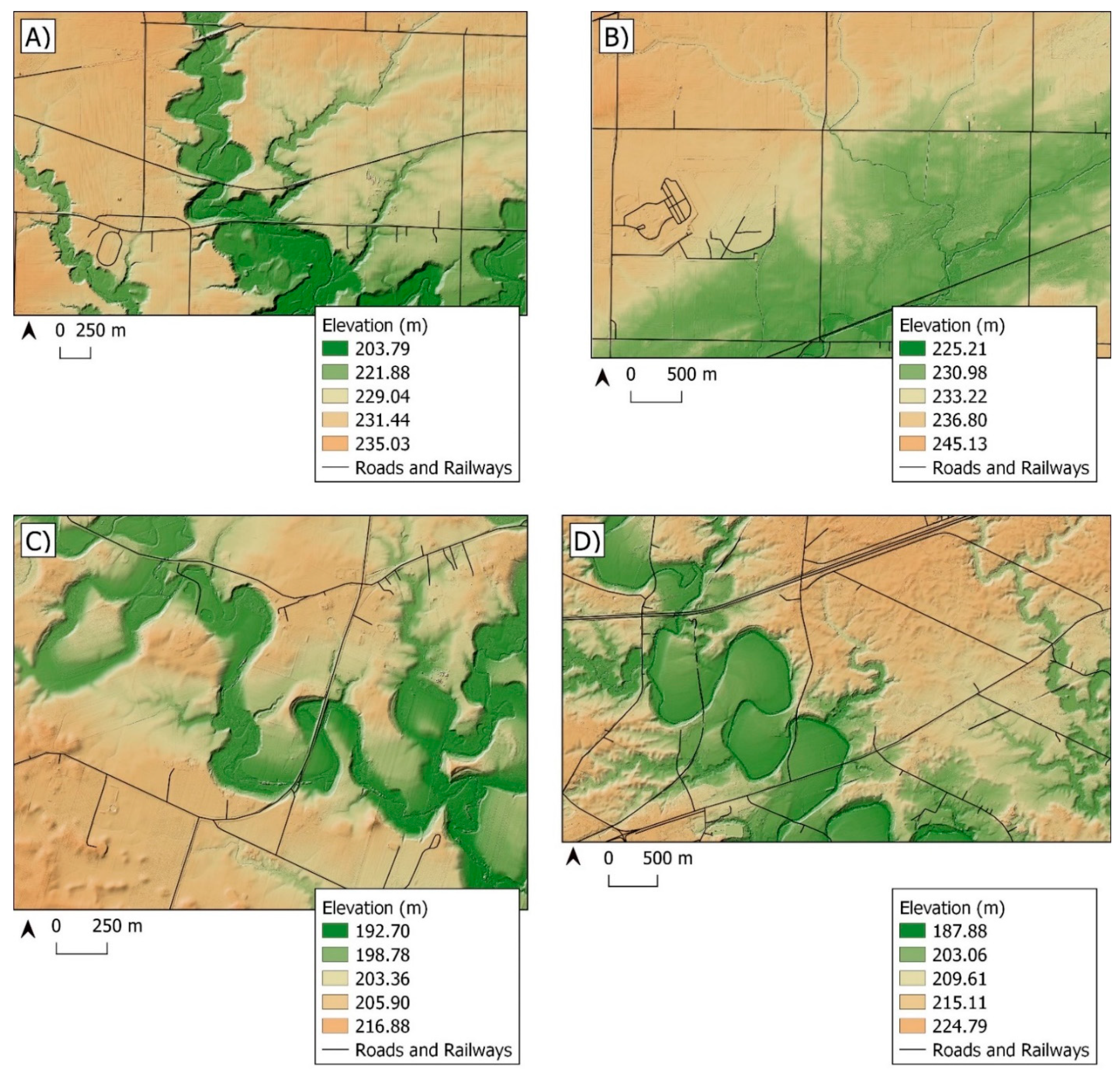
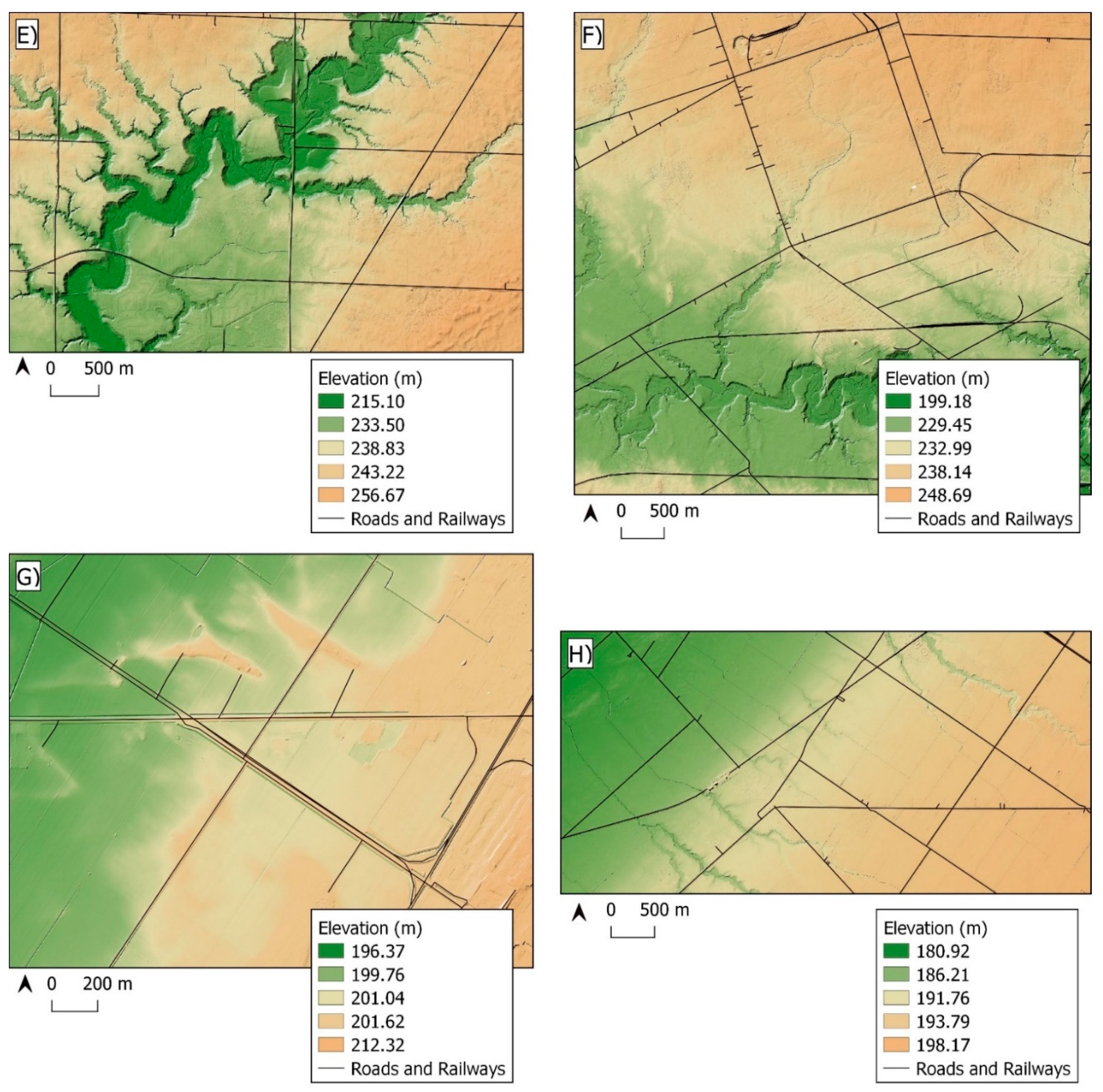
The method was tested on eight low-relief LiDAR DEMs representative of agricultural landscapes within southwestern Ontario, Canada (Figure 3, Table 2). The LiDAR point-cloud data were originally acquired by a 3rd party LiDAR provider on behalf of the Ontario Ministry of Agriculture, Food, and Rural Affairs (OMAFRA) and the Ontario Ministry of Natural Resources and Forestry (OMNRF). The point clouds were collected by the data provider using a Leica ALS70-HP sensor at an average density of 8 points/m2 starting in the fall of 2016 and ending in the spring of 2018 [27].
The LiDAR point clouds were interpolated to 0.5 m resolution bare-earth DEMs using the LidarTinGridding tool found in the WhiteboxTools geospatial analysis software [25]. The study sites range in relief from a minimum of 16.16 m at the McGregor Creek Test Site 1 to a maximum relief of 49.97 m at the Kettle Creek Test Site 2. Each study site was selected for exhibiting a variety of embankment morphologies. Transportation network vector data sets were obtained from the OMNRF and edited to include smaller embankments un-mapped in the original transportation network.

2.3. Algorithm Validation

Eight validation datasets were created by manually digitizing the mapped and un-mapped embankments in each study site, using hillshade images derived from the LiDAR DEMs, orthoimagery, and the transportation network vectors as guides. The digitized reference embankments were then rasterized.
To measure the algorithm accuracy, the derived embankment maps were compared to the reference embankment rasters using the recall, precision, and Pearson’s phi coefficient (PPC) metrics. These metrics are useful for evaluating the accuracy of a binary classification technique [28,29]. Recall (1) refers to the percentage of reference data that is correctly classified by the algorithm, and is calculated as:
R e c a l l = T P T P + F N
where TP is the number of cells classified as true positives (correctly classified embankment cells) and FN is the number of cells classified as false negatives. Precision (2) refers to the percentage of cells classified by the algorithm that are correct, and is calculated as:
P r e c i s i o n = T P T P + F P
where FP is the number of cells classified as false positives. Finally, the PPC (3) is a coefficient of correlation between observed and predicted binary classes and is functionally equivalent to the Matthews correlation coefficient widely used in bioinformatics and machine learning [30,31]. The PPC yields values between negative one and positive one, indicating perfect disagreement and perfect agreement, respectively, between observed and predicted classes. The PPC takes true negatives and class size into account, making this metric more robust than similar classification metrics such as the F1 score [28], and is calculated as:
P P C = T P T N F P F N ( T P + F P ) ( T P + F N ) ( T N + F P ) ( T N + F N )
where TN is the number of cells classified as true negatives.
In addition to accuracy, the tool’s computational efficiency was assessed. Once optimal parameter settings were found through experimentation, the tool was applied 10 times to each of the eight test data sets using constant parameter settings and the minimum processing times of each test set was recorded. Processing times excluded data input and output. All tests were performed on an i9-9980 computer system with eight processor cores and 64.0 GB of DDR4 memory.

3. Results

3.1. Algorithm Performance

The tool was applied to each of the eight study sites with varying parameter settings to determine the optimal settings for efficient algorithm performance (Table 3). Table 4 presents a summary of the performance metrics of the algorithm at each study site. The technique performed best on Catfish Creek Test Site 2, achieving a recall of 94.0%, a precision of 81.8%, and an PPC of 0.873. The algorithm showed the poorest performance on Kettle Creek Test Site 1, achieving a recall of 87.3%, a precision of 67.3%, and an PPC of 0.760. The algorithm achieved a recall greater than or equal to 90.0% for seven of the eight study sites, and an PPC greater than or equal to 80% for five of the eight study sites. The fastest processing time achieved by the algorithm was 1.4 s on the East Brantford Test Site 1, a 0.075 GB DEM. The slowest processing time measured during the tests was for the Kettle Creek Test Site 2, a 0.51 GB DEM, where the tool took 20.3 s to complete the embankment mapping.

3.2. Classification

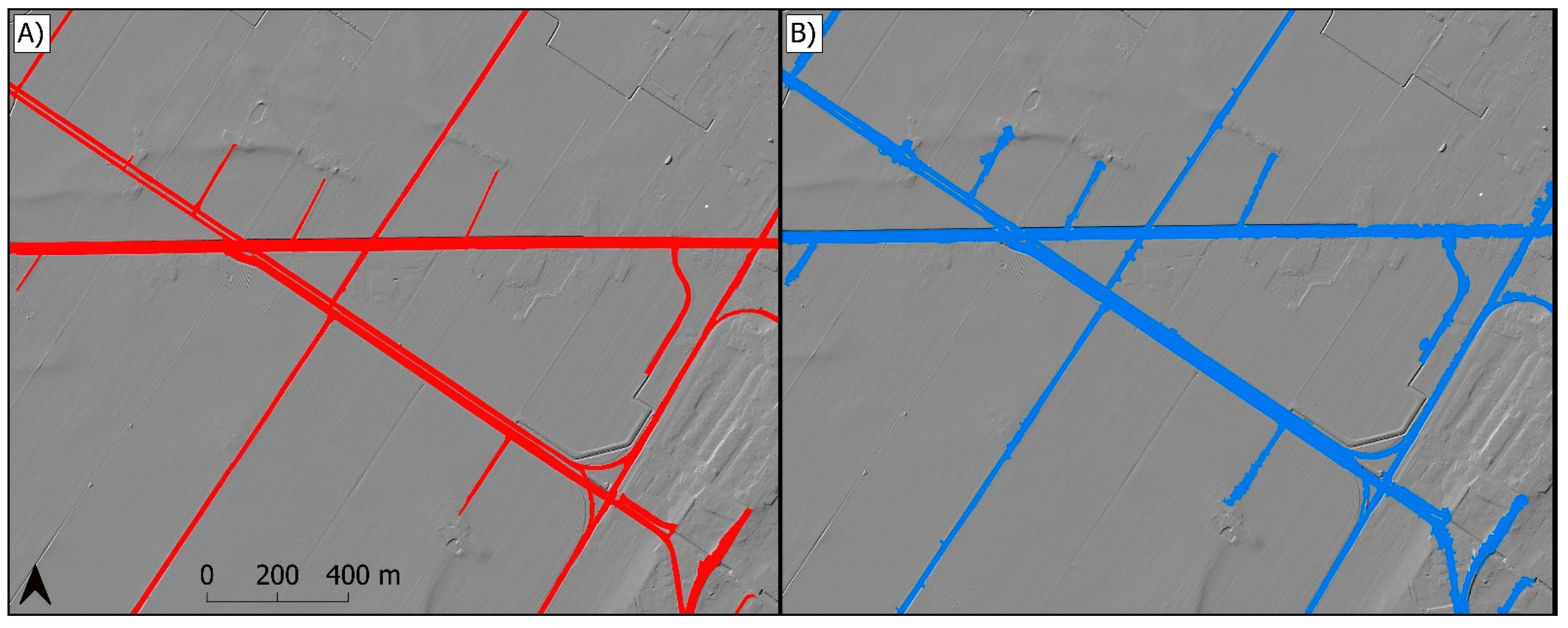
Figure 4 shows an example of all the transportation embankments identified by the embankment mapping tool for the McGregor Creek Test Site 1. The recall achieved for this site indicates that 96.5% of all reference embankment cells (Figure 4A) were correctly classified as embankment cells by the algorithm.
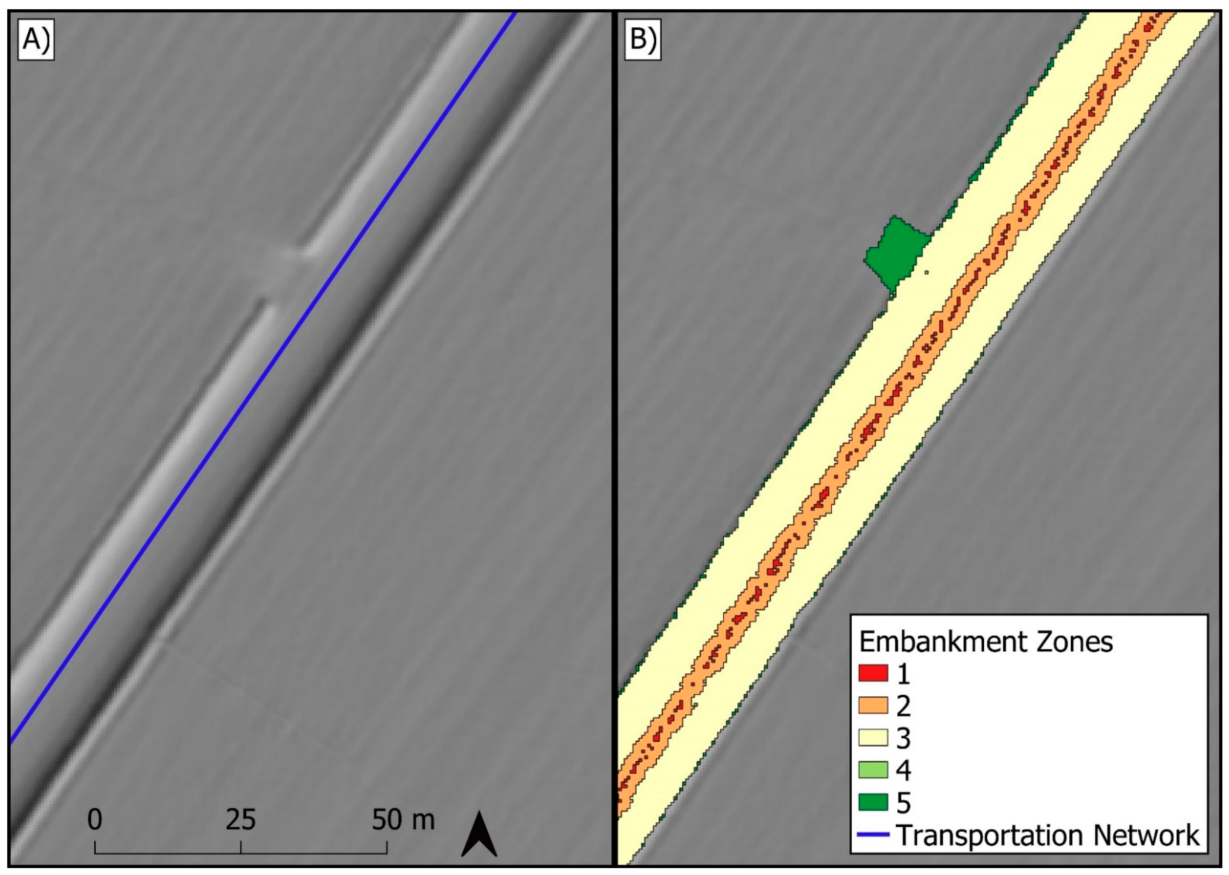
Figure 5 demonstrates the tool’s ability to identify ditch-lined embankments. Beyond Zones 1 and 2, corresponding to seed points and the level embankment surface width, respectively, most of the identified embankment region maps to Zone 3 cells.
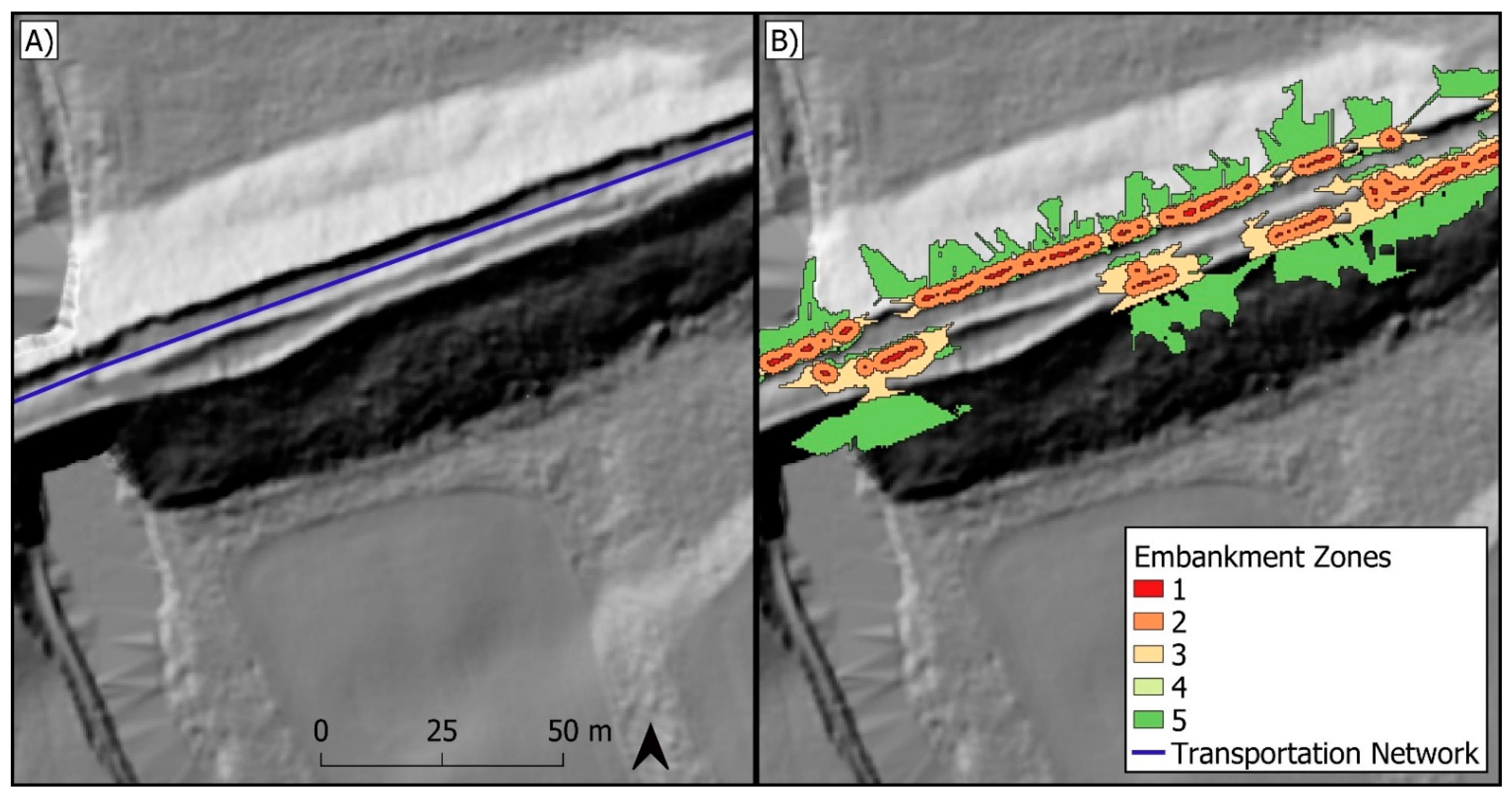
Figure 6 demonstrates the algorithm’s ability to identify embankments at valley crossings. These embankments have wide, steep sides without ditches that correspond to Zone 5 of the zonal embankment model (Figure 1). As expected, the sides of embankments at valley crossings are mapped as Zone 5 cells.
The algorithm’s inability to correctly classify embankments with an atypical morphology is demonstrated in Figure 7. This embankment at a valley crossing is an abandoned railway line that has been converted into a recreational trail. There are ridges to either side of the embankment surface that likely represent fencing or guard rails. The embankment mapping tool’s region-growing method struggled to grow beyond these lateral ridges and was unable to provide satisfactory coverage of the full embankment width. Furthermore, the seed-point placement algorithm frequently relocated seed points to the tops of the lateral ridges. Such atypical embankments were, however, rare within the study data sets.
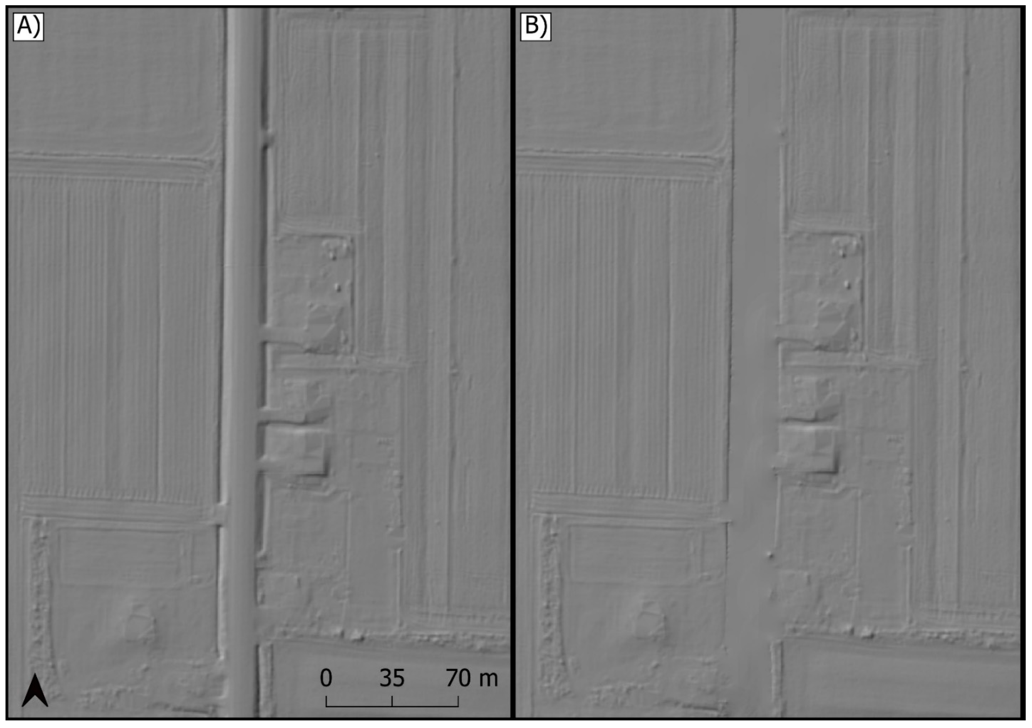
Figure 8 demonstrates the effect of removing mapped embankments and interpolating a surface in the data gaps left by the excised features. Data voids were filled using an inverse-distance weighted (IDW) interpolation technique.

4. Discussion

4.1. Embankment Classification

The tests produced high PPC and recall values, and moderate to high precision values. These results indicate that the embankment mapping algorithm identifies transportation embankments in LiDAR DEMs with moderate to high levels of accuracy. For most embankments in each study site, the algorithm correctly classifies reference embankment cells as embankment cells according to the zonal model of ditch-lined embankments and embankments at valley crossings developed in Figure 1.
Although Zone 5 of the zonal model of embankments corresponds to the sides of embankments at valley crossings, Zone 5 can be co-opted to map features such as driveways. The driveway in Figure 5B is mapped to Zone 5 because this feature extends beyond the typical embankment width while still sharing morphometric characteristics of the embankment surface. Since driveways could act as region spill-out points, being sites where the embankment is directly connected to the surrounding terrain beyond the drainage ditches, it is important to notice that the embankment region experienced minimal spill-out from the driveway. Thus, by finding optimal parameter settings, both satisfactory embankment classification and limited region spill out can be achieved.
While mapping precision was moderate to high in all tests, it was more than 10% lower on average than recall. It is hypothesized that the reduced precision is a result of the use of a less restrictive maximum embankment width parameter setting in testing. That is, a wider maximum embankment width setting allows the classified region to grow beyond the actual width of some ditch-lined embankments and spill into the surrounding landscape, increasing the number of false positives. However, a narrower maximum embankment width setting results in unsatisfactory classification of embankments at valley crossings, which are often much wider than ditch-lined embankments, reducing the number of true positives. Therefore, the algorithm’s performance is quite sensitive to the maximum embankment width parameter. It is suggested that a relatively large maximum embankment width setting be used, because satisfactory embankment classification with modest region spill-out should be preferred so that as few embankment cells as possible are left in the DEM once embankments have been removed.
The algorithm performs poorly when there is a mismatch between the morphology of a digital embankment and the embankment model morphologies of either a ditch-lined embankment or an embankment at a valley crossing (Figure 1). In Figure 7B, the lateral ridges representing fencing or guard rails confound the seed repositioning component of the algorithm regardless of the search distance used. This embankment also exhibits a rougher surface than most embankments because it is an unpaved recreational trail, which likely limits the effectiveness of the maximum upward elevation increment growth parameter. That is, if the variance in elevation is greater than the maximum upward elevation increment, the region will only grow into Zone 2 or Zone 5, as these zones do not depend on this parameter. However, such atypical embankment morphology was rare across all eight datasets (only one such location was found in all eight study sites). Other embankment morphologies, such as multi-lane highways with raised medians, do not present a problem for the algorithm because these features are represented with a vector line for each direction of travel rather than a single vector line for the entire feature.

4.2. Embankment Removal

The embankment map created by the tool can be used to remove embankments from a DEM for applications where the presence of embankments is undesirable. This can be accomplished by setting the mapped embankment cells to NoData in the output DEM, producing an embankment-less DEM. Once embankments have been removed, a surface approximating the terrain beneath embankments can be interpolated from the areas adjacent to the excised embankments.
The embankment mapping tool offers users the option to automatically perform the embankment removal and IDW surface interpolation. However, no single interpolation technique is suitable for all applications and all landscapes [32,33,34,35,36,37], and so the IDW interpolator used by the tool may not be optimal in all applications. In such cases, users should manually interpolate across mapped embankments using the interpolator most suited to the user’s data and application.

4.3. Algorithm Limitations

Although the embankment mapping method introduced in this paper demonstrates moderate to high accuracy for identifying embankments in fine-resolution DEMs, there are several limitations that can impact the use of the tool in a DEM pre-processing workflow.
1. Transportation network vectors often exclude small, un-mapped roads or long driveways represented in fine-resolution DEMs. Users must edit their transportation vectors to include these features if mapping and removal of the embankments of such features is required. Furthermore, some transportation vectors can be misaligned with embankments. While the seed repositioning component of the algorithm can mitigate this problem in many cases, if vectors are misaligned beyond a reasonable seed repositioning search distance, it is recommended that the user edit their vector data for better alignment. Thus, the algorithm is sensitive to the quality of the transportation network vector.
2. Typically, the robustness of region-growing methods is limited by the quality of seed points [38,39]. Although the seed repositioning component of the algorithm is generally robust, it can identify non-embankment cells as potential seed points even when a relatively small search distance is used, depending on the local topography. This is generally the case where the road vector is misaligned to the edge of the embankment and where the embankment is part of a larger roadcut. In the Kettle Creek 1 study site (the site with the poorest performance), a large number of road cuts caused many seed points to be assigned to non-embankment terrain and region growth into the surrounding terrain, reducing the recall and precision metrics for this site. This problem can often be solved by ensuring that the repositioning search distance is less than half of the typical embankment width, and by manual realignment of transportation vectors. The algorithm’s performance is therefore sensitive to the seed repositioning search distance parameter.
3. Embankments are better classified when parameter settings are less restrictive. Using relatively restrictive parameter settings to minimize region spill-out is problematic because embankment cells remaining in the DEM will result in localized elevation peaks once the data gaps left by the excised embankments are interpolated.
4. There may be a mismatch between the morphology of a digital embankment and the morphology of a ditch-lined embankment or an embankment at a valley crossing (Figure 1). Atypical embankment morphology, such as the recreational trail with fencing or guard rails in Figure 7, may be a result of DEM pre-processing errors or may represent real morphology. In such cases, inadequate embankment classification can occur.

5. Conclusions

Road and railway embankments are well represented in fine-resolution LiDAR DEMs. Modelled hydrological flow paths are impacted by the presence of embankments because remote sensing technologies are unable to capture the drainage culverts beneath embankments, and the embankments themselves interfere with the reconstruction of pre-embankment surfaces. Furthermore, the local topographic effects of embankments, particularly on the derivation of terrain attributes such as slope, reduce the accuracy of modelling applications such as predictive soil mapping, vegetation distribution mapping, and wetland mapping.
This paper presented a method for identifying embankments in LiDAR DEMs that relies on a region-growing operation. The algorithm begins by repositioning potential seed cells used for the region-growing operation to ensure satisfactory embankment classification when the input vector data is misaligned. The embankment region then grows using derived morphometric parameters including embankment slope, height, and width, classifying cells based on a zonal model of ditch-lined embankments and embankments at valley crossings.
The embankment mapping technique was applied to eight fine-resolution LiDAR DEMs representing largely agricultural areas of southwestern Ontario, Canada, and validated using manually digitized reference embankments. The results indicate that the technique demonstrated good computational efficiency and a moderate to high accuracy when applied to embankments that match the profiles of ditch-lined embankments and embankments at valley crossings. The tests showed that the method could correctly classify 87.3–96.5% of transportation embankment grid cells across study sites. The embankments mapped by the algorithm can be removed and a new surface interpolated as part of a DEM pre-processing workflow to improve the accuracy of modelling applications impacted by the presence of embankments in DEMs.

Author Contributions

Conceptualization, N.V.N. and J.B.L.; methodology, N.V.N. and J.B.L.; software, J.B.L. and N.V.N.; validation, N.V.N.; formal analysis, N.V.N. and J.B.L.; investigation, N.V.N. and J.B.L.; resources, J.B.L.; data curation, N.V.N.; writing—original draft preparation, N.V.N. and J.B.L.; writing—review and editing, N.V.N., J.B.L. and B.D.; visualization, N.V.N.; supervision, J.B.L. and B.D.; project administration, J.B.L.; funding acquisition, J.B.L. All authors have read and agreed to the published version of the manuscript.

Funding

This research was funded by a grant provided by the Natural Sciences and Engineering Research Council of Canada (NSERC; grant number 400317) and by a grant provided by the Ontario Ministry of Agriculture, Food, and Rural Affairs (OMAFRA; grant number 030500).

Institutional Review Board Statement

Not applicable.

Informed Consent Statement

Not applicable.

Data Availability Statement

The source data used in this research is available in a public repository and can be found at https://geohub.lio.gov.on.ca/datasets/776819a7a0de42f3b75e40527cc36a0a (accessed on 13 January 2021).

Acknowledgments

The authors would like to thank the contributions of the four anonymous reviewers. The authors would also like to thank Carys Owen for their efforts in the creation of the reference data sets used in the analysis of this work.

Conflicts of Interest

The authors declare no conflict of interest. The funders had no role in the design of the study; in the collection, analyses, or interpretation of data; in the writing of the manuscript, or in the decision to publish the results.

References

  1. Lindsay, J.B.; Dhun, K. Modelling surface drainage patterns in altered landscapes using LiDAR. Int. J. Geogr. Inf. Sci. 2015, 29, 397–411. [Google Scholar] [CrossRef]
  2. Lunardi, P. Embankment Formed by Preformed Collaborating Assemblable Elements, in Particular for Road or Railway Constructions, and Process. U.S. Patent No. 5,482,408, 9 January 1996. [Google Scholar]
  3. Wu, W.; Berhe, T.G.; Ashour, T. Embankments and dams. In Modern Earth Buildings; Woodhead Publishing: Cambridge, UK, 2012; pp. 538–558. [Google Scholar]
  4. Lidberg, W.; Nilsson, M.; Lundmark, T.; Ågren, A.M. Evaluating preprocessing methods of digital elevation models for hydrological modelling. Hydrol. Process. 2017, 31, 4660–4668. [Google Scholar] [CrossRef] [Green Version]
  5. Mäkinen, V.; Oksanen, J.; Sarjakoski, T. Automatic determination of stream networks from DEMs by using road network data to locate culverts. Int. J. Geogr. Inf. Sci. 2018, 33, 291–313. [Google Scholar] [CrossRef] [Green Version]
  6. Duke, G.D.; Kienzle, S.W.; Johnson, D.L.; Byrne, J.M. Improving overland flow routing by incorporating ancillary road data into Digital Elevation Models. J. Spat. Hydrol. 2003, 3. [Google Scholar] [CrossRef]
  7. Duke, G.D.; Kienzle, S.W.; Johnson, D.L.; Byrne, J.M. Incorporating ancillary data to refine anthropogenically modified overland flow paths. Hydrol. Process. 2006, 20, 1827–1843. [Google Scholar] [CrossRef]
  8. Thomas, I.A.; Jordan, P.; Shine, O.; Fenton, O.; Mellander, P.E.; Dunlop, P.; Murphy, P.N.C. Defining optimal DEM resolutions and point densities for modelling hydrologically sensitive areas in agricultural catchments dominated by microtopography. Int. J. Appl. Earth Obs. Geoinf. 2017, 54, 38–52. [Google Scholar] [CrossRef] [Green Version]
  9. Yu, F.; Harbor, J.M. The effects of topographic depressions on multiscale overland flow connectivity: A high-resolution spatiotemporal pattern analysis approach based on connectivity statistics. Hydrol. Process. 2019, 33, 1403–1419. [Google Scholar] [CrossRef]
  10. Zandbergen, P. Accuracy considerations in the analysis of depressions in medium-resolution lidar DEMs. Gisci. Remote Sens. 2010, 47, 187–207. [Google Scholar] [CrossRef]
  11. Lindsay, J.B. Efficient hybrid breaching-filling sink removal methods for flow path enforcement in digital elevation models. Hydrol. Process. 2016, 30, 846–857. [Google Scholar] [CrossRef]
  12. Stanislawski, L.; Brockmeyer, T.; Shavers, E. Automated road breaching to enhance extraction of natural drainage networks from elevation models through deep learning. Int. Arch. Photogramm. Remote Sens. Spat. Inf. Sci. Isprs Arch. 2018, 42, 671–678. [Google Scholar] [CrossRef] [Green Version]
  13. Florinsky, I.V.; Kuryakova, G.A. Influence of topography on some vegetation cover properties. Catena 1996, 27, 123–141. [Google Scholar] [CrossRef]
  14. Köthe, R.; Bock, M. Preprocessing of Digital Elevation Models–derived from Laser Scanning and Radar Interferometry–for Terrain Analysis in Geosciences. Proc. Geomorphometry 2009, 2, 155–161. [Google Scholar]
  15. McBratney, A.B.; Mendonça Santos, M.L.; Minasny, B. On digital soil mapping. Geoderma 2003, 117, 3–52. [Google Scholar] [CrossRef]
  16. Scull, P.; Franklin, J.; Chadwick, O.A.; McArthur, D. Predictive soil mapping: A review. Prog. Phys. Geogr. Earth Environ. 2003, 27, 171–197. [Google Scholar] [CrossRef] [Green Version]
  17. Hormese, J.; Saravanan, C. Automated Road Extraction from High Resolution Satellite Images. Procedia Technol. 2016, 24, 1460–1467. [Google Scholar] [CrossRef] [Green Version]
  18. Hu, X.; Tao, C.V.; Hu, Y. Automatic road extraction from dense urban area by integrated processing of high-resolution imagery and lidar data. Int. Arch. Photogramm. Remote Sens. Spat. Inf. Sci. 2004, 35 Pt B3, 288–292. [Google Scholar]
  19. Karnieli, A.; Meisels, A.; Fisher, L.; Arkin, Y. Automated Extraction and Evaluation of Geological Linear Features from Digital Remote Sensing Data Using a Hough Transform. Photogramm. Eng. Remote Sens. 1996, 62, 525–531. [Google Scholar]
  20. Lu, P.; Du, K.; Yu, W.; Wang, R.; Deng, Y.; Balz, T. A new region growing-based method for road network extraction and its application on different resolution SAR images. IEEE J. Sel. Top. Appl. Earth Obs. Remote Sens. 2014, 7, 4772–4783. [Google Scholar] [CrossRef]
  21. Quackenbush, L.J. A review of techniques for extracting linear features from imagery. Photogramm. Eng. Remote Sens. 2004, 70, 1383–1392. [Google Scholar] [CrossRef] [Green Version]
  22. Tupin, F.; Maitre, H.; Mangin, J.F.; Nicolas, J.M.; Pechersky, E. Detection of linear features in SAR images: Application to road network extraction. IEEE Trans. Geosci. Remote Sens. 1998, 36, 434–453. [Google Scholar] [CrossRef] [Green Version]
  23. Huang, X.; Cao, R.; Cao, Y. A Density-Based Clustering Method for the Segmentation of Individual Buildings from Filtered Airborne LiDAR Point Clouds. J. Indian Soc. Remote Sens. 2019, 47, 907–921. [Google Scholar] [CrossRef]
  24. Cormen, T.H.; Leiserson, C.E.; Rivest, R.L.; Stein, C. Introduction to Algorithms; MIT Press: Cambridge, MA, USA, 2009. [Google Scholar]
  25. Lindsay, J.B. WhiteboxTools User Manual. Available online: https://jblindsay.github.io/wbt_book/preface.html (accessed on 3 September 2020).
  26. Embankment Mapping.rs. Available online: https://github.com/jblindsay/whitebox-tools/blob/master/src/tools/terrain_analysis/embankment_mapping.rs (accessed on 29 April 2020).
  27. Ontario Ministry of Natural Resources and Forestry. User Guide Lidar Point Cloud (2016-18) LIO Dataset; Queen’s Printer for Ontario. 2019. Available online: https://geohub.lio.gov.on.ca/datasets/776819a7a0de42f3b75e40527cc36a0a (accessed on 3 September 2020).
  28. Chicco, D.; Jurman, G. The advantages of the Matthews correlation coefficient (MCC) over F1 score and accuracy in binary classification evaluation. BMC Genom. 2020, 21, 6. [Google Scholar] [CrossRef] [Green Version]
  29. Manning, C.; Raghavan, P.; Schütze, H. Introduction to Information Retrieval; Cambridge University Press: Cambridge, UK, 2008. [Google Scholar]
  30. Matthews, B.W. Comparison of the predicted and observed secondary structure of T4 phage lysozyme. Biochim. Biophys. Acta (BBA) Protein Struct. 1975, 405, 442–451. [Google Scholar] [CrossRef]
  31. Cramer, H. Mathematical Methods of Statistics; Princeton University Press: Princeton, NJ, USA, 1946. [Google Scholar]
  32. Arun, P.V. A comparative analysis of different DEM interpolation methods. Egypt. J. Remote Sens. Space Sci. 2013, 16, 133–139. [Google Scholar] [CrossRef] [Green Version]
  33. Bater, C.W.; Coops, N.C. Evaluating error associated with lidar-derived DEM interpolation. Comput. Geosci. 2009, 35, 289–300. [Google Scholar] [CrossRef]
  34. Doucette, P.; Beard, K. Exploring the capability of some GIS surface interpolators for DEM gap fill. Photogramm. Eng. Remote Sens. 2000, 66, 881–888. [Google Scholar]
  35. Guo, Q.; Li, W.; Yu, H.; Alvarez, O. Effects of topographic variability and lidar sampling density on several DEM interpolation methods. Photogramm. Eng. Remote Sens. 2010, 76, 701–712. [Google Scholar] [CrossRef] [Green Version]
  36. Liu, X.; Zhang, Z.; Peterson, J. Evaluation of the performance of DEM interpolation algorithms for LiDAR data. In Proceedings of the 2009 Surveying and Spatial Sciences Institute Biennial International Conference: Spatial Diversity (SSC 2009), Adelaide, Australia, 28 September–2 October 2009; pp. 771–780. [Google Scholar]
  37. Setianto, A.; Triandini, T. Comparison of Kriging and Inverse Distance Weighted (Idw) Interpolation Methods in Lineament Extraction and Analysis. J. Appl. Geol. 2015, 5, 21–29. [Google Scholar] [CrossRef]
  38. Khaloo, A.; Lattanzi, D. Robust normal estimation and region growing segmentation of infrastructure 3D point cloud models. Adv. Eng. Inform. 2017, 34, 1–16. [Google Scholar] [CrossRef]
  39. Vo, A.V.; Truong-Hong, L.; Laefer, D.F.; Bertolotto, M. Octree-based region growing for point cloud segmentation. ISPRS J. Photogramm. Remote Sens. 2015, 104, 88–100. [Google Scholar] [CrossRef]
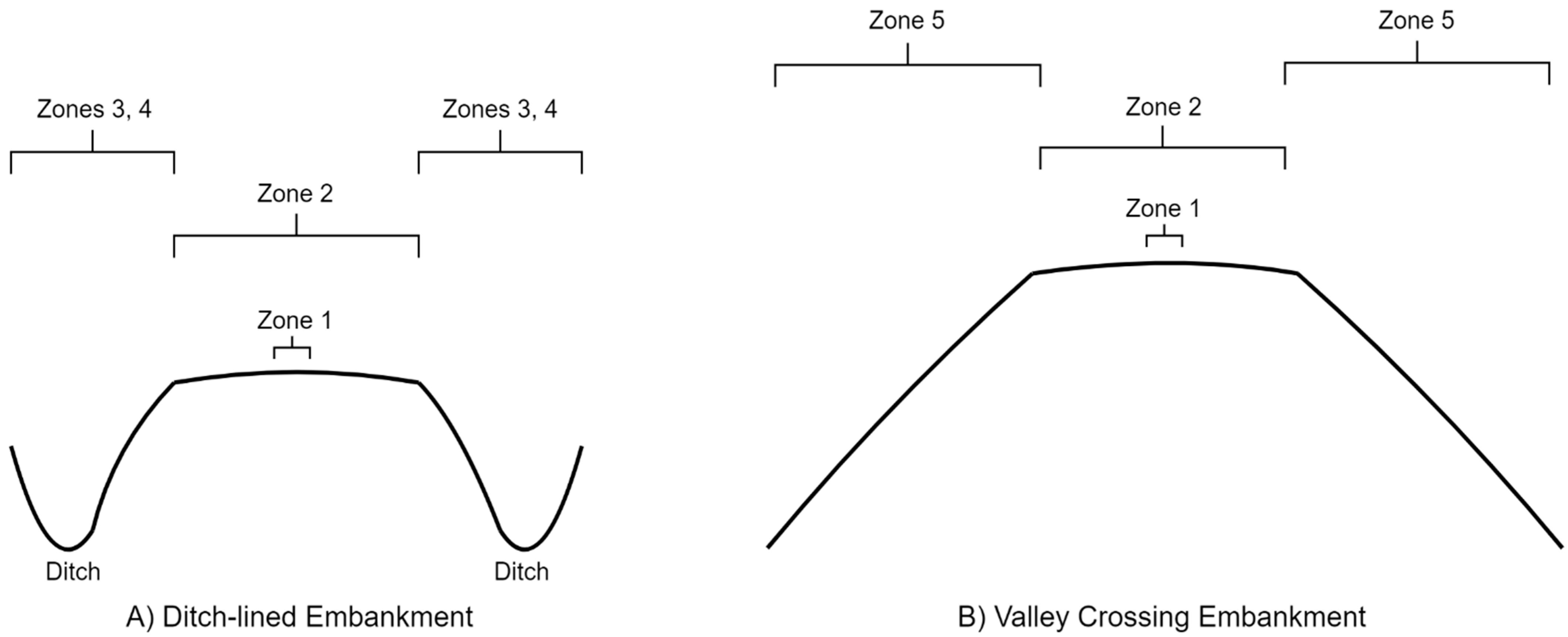
Figure 1. (A) Cross-sections of a ditch-lined embankment and corresponding embankment zones; (B) An embankment at a valley crossing and the corresponding embankment zones. These cross-sections are idealized conceptual profiles and not derived from real embankments.
Remotesensing 13 01308 g001
Figure 2. Seed point selection, parameter derivation, and region growing algorithm for the identification of embankments.
Remotesensing 13 01308 g002
Figure 3. Four of the eight study sites across southwestern Ontario, Canada. (A) The Catfish Creek 1 site; (B) The Catfish Creek 2 site; (C) the Brantford 1 site; (D) The Brantford 2 site. (E) The Kettle Creek 1 site; (F) The Kettle Creek 2 site; (G) the McGregor Creek 1 site; (H) The McGregor Creek 2 site. Only roads or railways on embankments have been included.
Remotesensing 13 01308 g003aRemotesensing 13 01308 g003b
Figure 4. (A) The digitized reference embankments of McGregor Creek Test Site 1; (B) The embankments classified by the algorithm.
Remotesensing 13 01308 g004
Figure 5. (A) A ditch-lined embankment; (B) The ditch-lined embankment identified by the algorithm. Notice the driveway that could potentially act as region spill-out point is mapped to Zone 5.
Remotesensing 13 01308 g005
Figure 6. (A) An embankment at a valley crossing; (B) The embankment at a valley crossing identified by the mapping. Zone 5 cells (dark green) correspond to the sides of embankment at a valley crossing as predicted by the zonal model of embankments.
Remotesensing 13 01308 g006
Figure 7. (A) Atypical morphology of an embankment at a valley crossing; (B) The embankment region classified by the algorithm.
Remotesensing 13 01308 g007
Figure 8. (A) A ditch-lined embankment; (B) The interpolated surface after the embankment was removed.
Remotesensing 13 01308 g008
Table 1. User-defined parameters required by the embankment mapping tool. All parameters are specified in map units, except for spill-out slope which is specified in degrees.
ParameterDescription
Seed repositioning search distanceSize of the neighbourhood to search around each transportation network cell
Minimum road widthWidth of the top of the level road or railway surface
Typical embankment widthMaximum width of a ditch-lined embankment
Maximum embankment widthMaximum width of an embankment at a valley crossing
Maximum typical embankment heightMaximum height of a ditch-lined embankment
Maximum upward elevation incrementMaximum elevation the embankment region is allowed to grow upwards
Spill-out slopeThreshold for the maximum absolute slope between a cell and its nearest seed
Table 2. Characteristics of the study site DEMs. Relief is the difference between the highest and lowest elevation in a dataset. Road/rail length refers to the total length of the edited transportation network vector, including all roads and railways on embankments.
Study SiteSize (Grid Cells)Relief (m)Road/Rail Length (km)
Catfish 142,636,00032.3521.57
Catfish 269,435,00020.4333.53
Brantford 119,791,00024.3310.52
Brantford 278,334,00038.1546.47
Kettle 176,184,00045.1126.23
Kettle 2134,723,00049.9769.22
McGregor 116,880,00016.1616.01
McGregor 242,636,00021.1632.89
Table 3. User-defined parameter settings for each of the eight study sites. SrchDist refers to the seed repositioning search distance. MinWidth refers to the minimum road width. TypWidth refers to the typical embankment width. MaxWidth refers to the maximum embankment width. MaxHght refers to the maximum embankment height. ElevInc refers to the maximum upward elevation increment. SpillSlope refers to the spill-out slope. All parameters are specified in map units, except for SpillSlope, which is specified in degrees.
Study SiteSrchDistMinWidthTypWidthMaxWidthMaxHghtElevIncSpillSlope
Catfish 110.04.015.035.01.00.0052.0
Catfish 210.05.015.025.01.00.0054.0
Brantford 15.05.015.030.01.00.0054.0
Brantford 25.06.025.035.01.00.056.0
Kettle 15.06.025.040.01.00.054.0
Kettle 23.06.025.040.02.00.054.0
McGregor 115.02.020.040.02.00.054.0
McGregor 28.04.020.035.02.00.054.0
Table 4. Performance metrics of the embankment identification algorithm at each study site. Processing time was measured as the minimum processing time of 10 test runs and excludes data input and output.
Study SiteProcessing Time (s)Recall (%)Precision (%)PPC
Catfish 14.690.470.70.792
Catfish 26.394.081.80.873
Brantford 11.490.375.50.820
Brantford 212.590.070.30.786
Kettle 16.687.367.30.760
Kettle 220.391.878.80.841
McGregor 12.696.578.10.859
McGregor 27.893.680.30.862
Publisher’s Note: MDPI stays neutral with regard to jurisdictional claims in published maps and institutional affiliations.