Quality Assessment of TanDEM-X DEMs, SRTM and ASTER GDEM on Selected Chinese Sites

Abstract

Digital elevation models (DEMs) are the basic data of science and engineering technology research. SRTM and ASTER GDEM are currently widely used global DEMs, and TanDEM-X DEM, released in 2016, has attracted users’ attention due to its unprecedented accuracy. These global datasets are often used for local applications and the quality of DEMs affects the results of applications. Many researchers have assessed and compared the quality of global DEMs on a local scale. To provide some additional insights on quality assessment of 12- and 30-m resolution TanDEM-X DEMs, 30-m resolution ASTER GDEM and 30-m resolution SRTM, this study assessed differences’ performance in relation to not only geographical features but also the ways in which DEMs have been created on selected Chinese sites, taking ICESat/GLAS points with 14-cm absolute vertical accuracy but size of 70-m diameter and 12-m resolution TanDEM-X DEM with less than 10-m absolute vertical accuracy as the reference data for comprehensive quality evaluation. When comparing the three 30-m DEMs with the reference DEM, an improved Least Z-Difference (LZD) method was applied for co-registration between models, and Quantile–Quantile (Q-Q) plot was used to identify if the DEM errors follow a normal distribution to help choose proper statistical indicators accordingly. The results show that: (1) TanDEM-X DEMs have the best overall quality, followed by SRTM. ASTER GDEM has the worst quality. The 12-m TanDEM-X DEM has significant advantages in describing terrain details. (2) The quality of DEM has a strong relationship with slope, aspect and land cover. However, the relationship between aspect and vertical quality weakens after data co-registration. The quality of DEMs gets higher with the increasing number of images used in the fusion process. The quality in where slopes opposite to the radar beam is the worst for SRTM, which could provide a new perspective for quality assessment of SRTM and other DEMs whose incidence angle files are available. (3) Systematic deviations can reduce the vertical quality of DEM. The differences have non-normal distribution even after co-registration. For researchers who want to know the quality of a DEM in order to use it in further applications, they should pay more attention to the terrain factors and land cover in their study areas and the ways in which the DEM has been created.

1. Introduction

Digital elevation models (DEMs) and terrain variables derived from DEMs (e.g., slope and aspect) are the basic data of science and engineering technology research. They play a necessary role in geomorphology [1], volcanology [2], glacier mass balance [3], flooding modeling [4], climatic modeling [5], etc. DEMs are now primarily generated using remote sensing techniques because of the benefits that fewer people can map a large spatial area at a lower cost [6]. Remote sensing techniques include photogrammetry, Interferometric Synthetic Aperture Radar (InSAR) and Light Detection And Ranging (LiDAR) [7].

Errors of DEM can propagate throughout the data processing in subsequent investigations they are used in and may adversely affect the accuracy of the results [8]. Therefore, it is very important to understand the quality of DEM to be used for certain applications [9]. At present, many agencies have released global DEM products, which can provide topographic information for researchers. These distributing organizations give the global accuracy of DEM products, which cannot represent the quality in the local area because the quality of DEM varies on a regional scale. Hence, the quality of DEMs should be quantitatively evaluated and used with caution in the local area [10]. Shuttle Radar Topography Mission (SRTM) DEM [11] and Advanced Space Borne Thermal Emission and Reflection Radiometer Global Digital Elevation Model (ASTER GDEM) [12] are the most commonly used global DEMs. Many scientific studies have reported the quality of these two DEMs in local regions [13,14,15,16,17]. TerraSAR-X add-on for Digital Elevation Measurement (TanDEM-X) DEM, released in September 2016, has attracted users’ attention due to its unprecedented geometric resolution, precision and accuracy as a global DEM product [18,19]. It resulted in three types of data with resolutions of 12, 30 and 90 m, respectively. Before the final TanDEM-X DEM was released, the German Aerospace Agency (DLR) released TanDEM-X intermediate DEM (IDEM). The biggest difference between IDEM and the final DEM is that IDEM was generated only based on the data obtained in the first year, which means that most areas are only covered once. There has been some research on the quality assessment of TanDEM-X IDEM and the final TanDEM-X DEM product. The research used RTK-GNSS ground measurement points [20], ICESat data [21], globally distributed GPS points [22], local DEMs [23], LiDAR DEM [24] or high-quality DSM derived from small footprint airborne LiDAR [25] as the reference data to assess the vertical accuracy of TanDEM-X IDEM [20,23] or TanDEM-X DEM [21,22,24,25] globally [21,22] or in local study area [20,23,24,25] with different altitudes, topography and vegetation [26,27,28,29,30,31,32]. The researchers also compared the obtained accuracy with other DEMs such as SRTM and ASTER GDEM. To assess a DEM’s accuracy, the accuracy of the reference should be at least three times better than that of the DEM to be assessed [14]. The references the above studies used could satisfy the accuracy requirements. When there was no very high accuracy reference data, Grohmann et al. [33] used the 12-m resolution TanDEM-X DEM with higher accuracy among the DEMs as the reference to assess the differences’ performance of 30-m resolution TanDEM-X DEM, ASTER GDEM, SRTM and ALOS AW3D DEM on selected Brazilian sites. Although they could not get the exact accuracy of the assessed DEMs, they could still provide insights into these DEMs’ quality, through the comparison of differences’ performance between elevation models.

These existing studies on the quality assessment of the 12- and 30-m TanDEM-X DEM product are rare in local areas of China. Keys et al. [28] used the result of catchment delineations obtained using 12-m TanDEM-X DEM as the reference to compare the results obtained using SRTM, ACE2 and ASTER GDEM in Nam Co, China. These existing studies also paid attention to the relationship between DEM’s quality and geographical features. In the analysis of the factors that affect the quality of DEM, researchers have carried out a large number of studies on the relationship between the quality and slope, aspect and land cover [13,14,24,34]. However, most of the studies analyze each factor independently, omitting the combined influence of the factors on the quality. Satge et al. [14] assessed the quality of DEM under different land cover where the slope was within 0–2° and 10–15°. Zhang et al. [34] found that the main factor affecting the quality of DEM was slope among slope, aspect and land cover. Besides, the ways in which DEMs have been created are also important to DEMs’ quality. TanDEM-X DEM, ASTER GDEM and SRTM were created from the fusion of many observations. Hu et al. [35] evaluated the influence of stack numbers on the quality of ASTER GDEM. Gdulová et al. [25] conducted a similar exploration of TanDEM-X DEM. TanDEM-X DEM and SRTM were generated from the InSAR technology, so the local incidence angle may impact the quality of the final DEMs as the geometry of the incidence angle strongly influences the quality of the reflected radar beam. Kolecka et al. [15] assessed the accuracy of SRTM X-band DEM in relation to radar beam geometry.

There are two main methods for evaluating the accuracy of DEMs currently [14]: comparing the assessed DEM (i.e., the DEM to be assessed) with higher accuracy points and DEMs, respectively. When taking a DEM as the reference, the assessed DEMs need to be registered with the reference DEM because there exist systematic offsets between the models in both horizontal and vertical directions due to the effect of sensor errors, the orientation bias of reference ellipsoids and topographic relief [35]. Some disadvantages of the related studies on co-registration were that the registration accuracy depended on the search step distance because of indirect computation [13,23], only the existence of translations was considered [13,15,23,30,35,36] or the co-registration procedure relied on manual recognition [16].

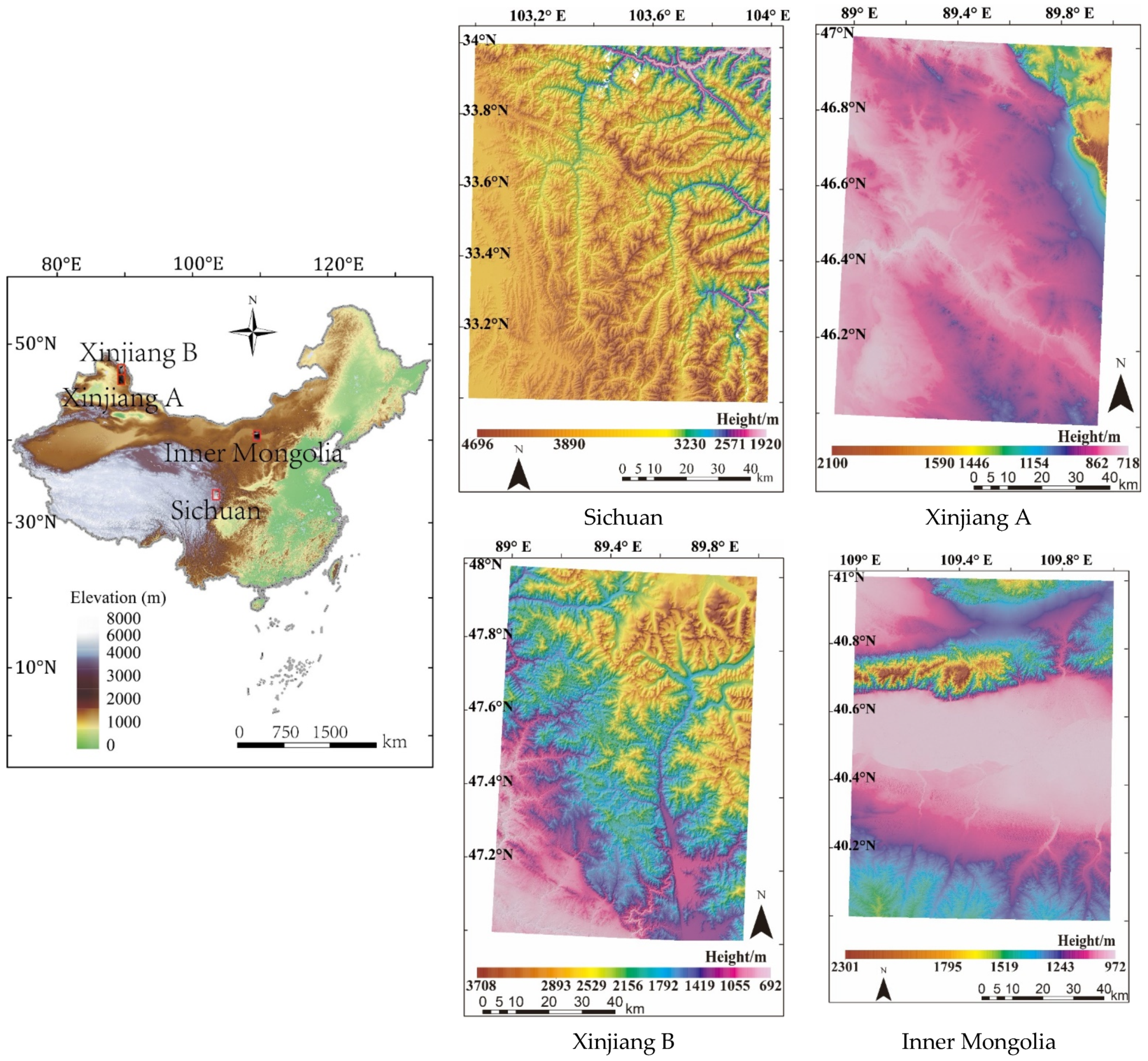
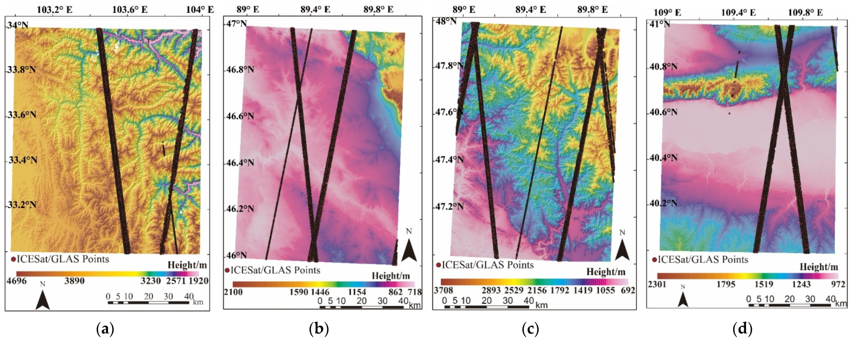
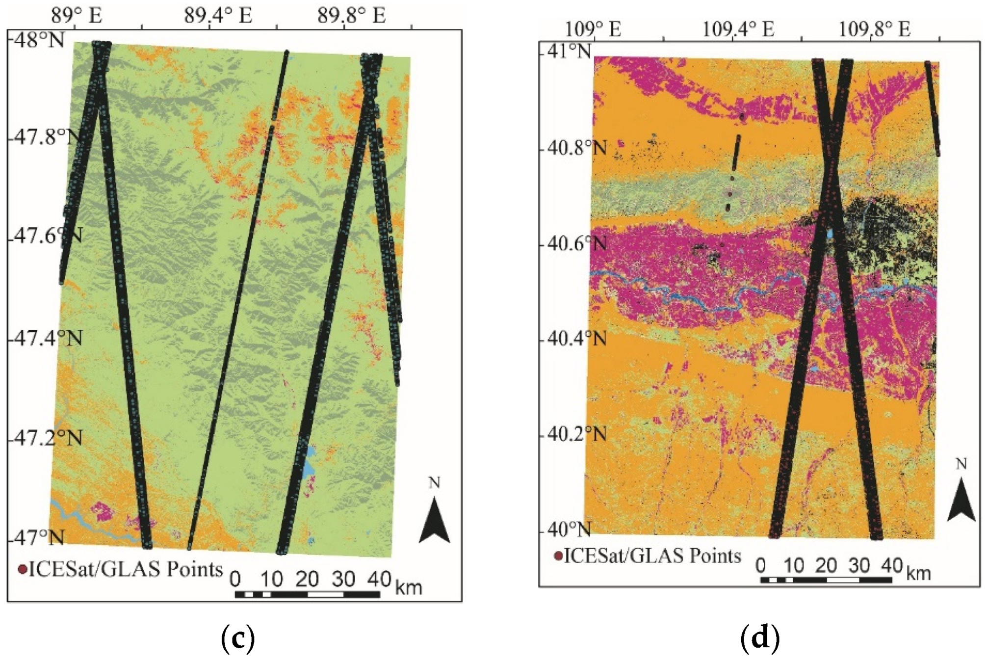
Aiming to the limitations of the existing studies on quality assessment of the DEMs, the objective of this article is to provide some additional insights on the quality assessment of TanDEM-X DEMs, ASTER GDEM and SRTM. We selected study areas in China because there is a necessity to test whether the assessed results are special in China. Due to the limit of the conditions, we could not obtain the ground truth data. High-resolution and high-accuracy data are almost classified in every country. It is very hard to obtain, especially in China. Thus, this study is not the traditional accuracy assessment of the DEMs, but the quality assessment. DEMs’ quality includes many aspects, not only the absolute accuracy but also differences’ performance in relation to various influencing factors, which is exactly what this article studies. The consistency between these DEMs and the reference data can indicate the quality. The higher is the accuracy of the reference data, the better, so that our results could provide more convincing guidance on DEMs’ quality for related application researchers. As a result, ICESat/GLAS points with 14-cm absolute vertical accuracy [37] were selected as the reference points. It should be noted that one ICESat/GLAS point has a diameter of 70 m on the ground, which is larger than the resolution of most DEMs, and the center spacing of adjacent points on the same track is about 172 m [37]. Moreover, the accuracy of ICESat/GLAS points in mountainous regions is not high [25]. Due to the small number, non-uniform distribution and lack of describing the terrain details of ICESat/GLAS points in the wide range of the area [22], taking a high-resolution and high-accuracy DEM with continuous and complete coverage as the reference to assess the quality of DEMs is also suitable. The 12-m resolution TanDEM-X DEM with less than 10 m absolute vertical accuracy [21] is the best we could utilize at this time. More specific goals of this article are as follows: (1) We assess and compare the vertical quality of 12- and 30-m resolution TanDEM-X DEM, 30-m resolution ASTER GDEM and 30-m resolution SRTM DEM on four selected Chinese sites; analyze the quality in terms of slope, aspect and landcover; control the variable of the slope when analyzing the relationship between land cover and quality; analyze the quality in terms of the number of images used in the fusion process for generating the final DEMs; and analyze the quality in terms of local incidence angle of SRTM C-band DEM for the first time, trying to provide a new perspective for quality assessment of SRTM and other DEMs whose incidence angle files are available. (2) We use an improved Least Z-Difference (LZD) method [38] which considers nine transformation parameters that may exist between two DEMs to accomplish the co-registration procedure. (3) We use a Quantile–Quantile (Q-Q) plot to identify if the DEM errors follow a normal distribution and choose proper statistical indicators accordingly.

2. Materials

2.1. Study Area

Four areas, each of which is a 1° × 1° tile, were chosen as study areas (Figure 1) in China based on two main criteria [32]: (1) the availability of the 12- and 30-m TanDEM-X DEM, as they are not openly available; and (2) the diversity of the terrain slope and the land cover, as they are the main factors known to influence DEMs’ quality. Thus, we chose these four study areas because the TanDEM-X DEMs were available and there were different topographic conditions (flat, hilly and mountainous areas) coexisting with various land cover types, making these areas suitable for a comprehensive DEM quality evaluation (

Table 1. Study area information.

Study Area	Geolocation	Height	Mean Slope	Major Land Cover	Climate
Sichuan	33° N–34° N, 103° E–104° E	1920 m–4696 m	28°	Forest	Plateau cold zone humid monsoon climate
Xinjiang A	46° N–47° N, 89° E–90° E	718 m–2100 m	4°	Bareland	Temperate continental climate
Xinjiang B	47° N–48° N, 89° E–90° E	692 m–3708 m	21°	Grassland	Temperate continental climate
Inner Mongolia	40° N–41° N, 109° E–110° E	972 m–2301 m	7°	Bareland	Temperate continental climate

). We named the study areas after the province where they are located. The study areas of Xinjiang A and Xinjiang B are adjacent. Each study area contains a small or most mountainous region. Most areas of Sichuan are high mountains. About 56% of Sichuan is covered by forest and about 40% is covered by cropland/grassland/bareland. There are large mountainous areas in the northeast of Xinjiang B. About 16% of Xinjiang B is covered by forest and about 74% is covered by cropland/grassland/bareland. There are small mountainous areas in the northeast of Xinjiang A. About 91% of Xinjiang A is covered by cropland/grassland/bareland. There are small and long mountainous areas in the north of Inner Mongolia. About 86% of Inner Mongolia is covered by cropland/grassland/bareland, about 3% is covered by forest and about 2% is covered by shrubland.

2.2. Elevation Data

Table 2. Characteristics of the elevation data used in this study.

Dataset	Imaging System	Pixel Spacing	Horizontal Datum/Vertical Datum	Absolute Vertical Accuracy	Relative Vertical Accuracy
TanDEM-X DEM	InSAR X band	0.4 arcsec (~12 m)	WGS84/WGS84	<10 m (LE90)	2 m (Slope ≤ 20%) 4 m (Slope > 20%)
		1 arcsec (~30 m)			\
SRTM	InSAR C band	1 arcsec (~30 m)	WGS84/EGM96	<16 m (LE90)	<10 m (LE90)
ASTER GDEM	Optical	1 arcsec (~30 m)	WGS84/EGM96	<20 m (LE95)	12.1 m
ICESat/GLAS	LiDAR	172 m	TOPEX/POSEIDON	14 cm	\

shows the characteristics of the elevation data used in this study.

TerraSAR-X add-on for Digital Elevation Measurements (TanDEM-X) mission is a constellation of two satellites with almost identical design parameters, flying in a close orbit formation with a baseline of 250–500 m and acquiring radar images of the Earth surface at high spatial resolution [21,39,40,41,42]. The 12-m resolution TanDEM-X DEM, the main product of the mission, is expected to go beyond the quality of global DEMs available so far with an unprecedented geometric resolution, precision and accuracy [18,19]. The configuration of the sensors and orbit allowed across-track and along-track interferometry. The mission accomplished complete imaging of Earth at least twice, with additional coverage in areas of complex topography, including the repositioning of the orbits to avoid radar shadowing in mountainous terrains [19,33,43,44]. Thus far, the data acquired during the mission between December 2010 and January 2015 resulted in three global datasets [25]: (1) TanDEM-X DEM produced by the DLR at a 0.4 (~12 m) and 1 arcsec (~30 m) resolution released in September 2016, which are available for scientific use (the 30-m resolution DEM was resampled from 12-m resolution DEM using the moving-window smoothing process); (2) WorldDEM from Airbus Defense and Space for commercial use at a 12-m resolution; and (3) freely available TanDEM-X DEM at 90-m resolution. We used the 12- and 30-m resolution TanDEM-X DEM provided by the DLR.

The Shuttle Radar Topography Mission (SRTM) was a cooperation among NASA, the U.S. National Geospatial-Intelligence Agency (NGA), U.S. Department of Defense (DoD), DLR and the Agenzia Spaziale Italiana (ASI, Italy) [33]. The shuttle carrying two SAR antennas with a baseline of 60 m can acquire radar images of the Earth surface simultaneously. Farr et al. [11] gave a detailed review of the SRTM mission. The data were acquired during 11 days in February 2000. The C band system (5.6 cm, SIR-C) and X band system (3.1 cm, X-SAR) operated during the mission, with the C radar generating a continuous mapping coverage and the X radar generating data along discrete swaths 50 km wide [11]. The SRTM data used in this study are from the C band system. In 2015, the 1 arcsec resolution (~30 m) SRTM V3 data in China was publicly released, which was used in this study. It was downloaded from the website (http://earthexplorer.usgs.gov/ (accessed on 2 January 2015)).

The Advanced Spaceborne Thermal Emission and Reflection Radiometer (ASTER) sensor was launched in December 1999 onboard the Terra satellite. It can generate along-track stereoscopic images on the Near Infra-Red wavelength (0.78–0.86 μm) [45]. In 2019, the 1 arcsec resolution (~30 m) ASTER GDEM V3 data were publicly released by the NASA Jet Propulsion Lab (JPL) and Japan’s Ministry of Economy, Trade, and Industry (METI), which was used in this study. It was downloaded from the website (https://search.earthdata.nasa.gov/ (accessed on 5 August 2019)).

It should be noted that the DEMs used in this study refer to Digital Surface Models (DSM). This is due to the weak penetration of TanDEM-X DEM and SRTM radar signals in dense vegetation and the sensitivity to the canopy of optical images used for generating ASTER GDEM.

In January 2003, Ice, Cloud, and land Elevation Satellite (ICESat) was launched by NASA. The Geo-science Laser Altimetry System (GLAS) carried on the satellite is mainly used to measure the height of the ice cover and its changes over time, the shape of clouds and aerosols, the height of land and the thickness of vegetation and the thickness of sea ice [46]. GLAS adopts the nadir direction observation mode. The laser pulse can form a spot with a diameter of 70 m on the ground, and the center spacing of adjacent laser spots on the same track is about 172 m [37]. At present, the standard ICESat/GLAS data products released by the National Snow and Ice Data Center (NSIDC) have 15 categories. GLAH14 is the altimetry data of the land surface reproduced from GLAH05 and GLAH06. Compared with the current DEMs, GLAH14 has higher accuracy. Thus, it is often used as the reference data for quality assessment of DEMs. This ICESat/GLAS GLAH14 was used in this study. It was downloaded from the website (https://nsidc.org/data/GLAH14/versions/34 (accessed on 1 August 2017).

2.3. Land Cover

Gong et al. applied the training sample set collected in 2015 to Sentinel-2 images acquired in 2017 to produce a 10-m resolution global land cover map, FROM-GLC10, with random forest classifier [47]. The dataset has 10 classes, namely cropland, forest, grassland, shrubland, wetland, water, tundra, impervious surface, bareland and snow/ice, with an overall accuracy of 72.76%. This dataset was used as ancillary data to assist our assessment. It was downloaded from the website (http://data.ess.tsinghua.edu.cn/fromglc10_2017v01.html (accessed on 8 March 2019).

3. Methods

There are two main methods for evaluating the accuracy of DEMs currently [14]. One is comparing the DEM with higher accuracy points, such as the GPS data and elevation control points collected from a large-scale topographic map. The accuracy of the reference points should be at least three times better than that of the DEM to be assessed. Another is comparing the DEM with higher accuracy DEMs, such as the DEM data generated by large-scale topographic maps, LiDAR DEMs and other higher-accuracy DEMs. Due to the lack of ground truth data, we cannot assess the absolute vertical accuracy of the DEMs in this study. We aim to assess differences’ performance to explore the consistency between the assessed DEMs and the reference data. The consistency can also reflect the quality of DEMs under the circumstance that the reference data is better than the assesses DEMs. Moreover, we can still borrow the above ideas for evaluating the accuracy of DEMs to assess DEMs’ quality in this study.

ICESat/GLAS GLAH14 points with 14-cm absolute vertical accuracy but size of 70-m diameter were chosen as the reference points to assess and compare the vertical quality of TanDEM-X DEM with a pixel size of 12 and 30 m and ASTER GDEM, SRTM with a pixel size of 30 m. It is also should be noted that the vertical accuracy of ICESat/GLAS points in mountainous regions is not high. Due to the small number, non-uniform distribution and lack of describing the terrain details of ICESat/GLAS points in the wide range of the study area, taking a high-resolution and high-accuracy DEM with continuous and complete coverage as the reference to assess the quality of DEMs is also suitable. Thus, 12-m resolution TanDEM-X DEM with less than 10 m absolute vertical accuracy, which is the best we could utilize at this time, was chosen as the reference DEM of the other three DEMs with a pixel size of 30 m to perform a model-to-model comparison. Previous studies [28,33,48] have also used the 12-m TanDEM-X DEM as the reference to test the height quality and the performance in applications of many independent datasets. Through the analysis of the height differences’ performance between the assessed DEMs and the reference, we could evaluate the quality of the DEMs. Figure 2 describes the general workflow of this study.

3.1. Data Preprocessing

Since the horizontal and vertical datums of these elevation data are different (Table 2), they need to be unified [15]. The plane position difference of the WGS84 ellipsoid and the Topex/Poseidon ellipsoid is very small [49,50], so the difference in the vertical direction is mainly considered [51]. The WGS84 ellipsoid, the native vertical datum of TanDEM-X DEM, was selected as the vertical reference datum in this study.

The vertical datum of ASTER GDEM and SRTM is the EGM96 geoid. The deviations of the EGM96 from the WGS84 ellipsoid provided by GAMMA software were used to convert the vertical datums of these two DEMs. The vertical datum of ICESat/GLAS points is the Topex/Poseidon ellipsoid. The MATLAB tool provided by NSIDC was used to read the ICESat/GLAS data, and the parameter d_deltaEllip was used to convert the vertical datum from the T/P ellipsoid to the vertical reference datum. Two quality control parameters provided by NSIDC were selected to remove low-quality ICESat/GLAS points. The first parameter elev_use_flg indicates whether the elevation value should be used or not, and only the data with a value of 0 were selected. The second parameter sat_corr_flg indicates whether saturation phenomenon occurred during the acquisition and if it was corrected, and only the non-saturated points were selected. Moreover, the ICESat/GLAS points whose absolute difference with other DEMs is greater than 50 m were removed. We kept the 50-m threshold to eliminate the gross errors of the ICESat/GLAS points so as to ensure a high-quality database [52], especially considering that the accuracy of ICESat/GLAS points in mountainous regions is not high [25]. Finally, all elevation data were projected to the UTM coordinate system using ArcGIS [53].

3.2. Data Co-Registration

When performing the model-to-model comparison, the assessed DEMs need to be registered with the reference DEM. Although the datum unifying is implemented, there still exist systematic offsets between the assessed DEMs and the reference DEM in both horizontal and vertical directions due to the effect of sensor errors, the orientation bias of reference ellipsoids and topographic relief [35]. An improved Least Z-Difference (LZD) method was applied to data co-registration in this study. Generally, the DEM co-registration model can be expressed by Equation (1) [38]:

$$\left[\begin{array}{c}X\\ Y\\ Z\end{array}\right] = \left[\begin{array}{c}{T}_X\\ T_Y\\ T_Z\end{array}\right] + \mathrm{M} \times \mathrm{R}\left[\begin{array}{c}x\\ y\\ z\end{array}\right],$$

(1)

where X, Y and Z are the three-dimensional coordinates of the reference DEM, respectively. x, y and z are the three-dimensional coordinates of the assessed DEM, respectively. $T_X$, $T_Y$ and $T_Z$ are the translations in three-dimensional direction of the assessed DEM, respectively. $\mathrm{M}$ is the three-dimensional scale factor of the assessed DEM. R is the rotation matrix (Equation (2)).

$$\mathrm{R}=\left[\begin{array}{ccc}r11& r12& r13\\ r21& r22& r23\\ r31& r32& r33\end{array}\right],$$

(2)

where r11 = cos${\theta }_y$ × cos${\theta }_z$, r21 = cos${\theta }_x$ × sin${\theta }_z$ + sin${\theta }_x$ × sin${\theta }_y$ × cos${\theta }_z$, r31 = sin${\theta }_x$ × sin${\theta }_z$ − cos${\theta }_x$ × sin${\theta }_y$ × cos${\theta }_z$, r12 = −cos${\theta }_y$ × sin${\theta }_z$, r22 = cos${\theta }_x$ × cos${\theta }_z$ − sin${\theta }_x$ × sin${\theta }_y$ × sin${\theta }_z$, r32 = sin${\theta }_x$ × cos${\theta }_z$ + cos${\theta }_x$ × sin${\theta }_y$ × sin${\theta }_z$, r13 = sin${\theta }_y$, r23 = −sin${\theta }_x$ × cos${\theta }_y$ and r33 = cos${\theta }_x$ × cos${\theta }_y$. ${\theta }_x$, ${\theta }_y$ and ${\theta }_z$ are three rotation angles of the assessed DEM around three axes, respectively.

The co-registration process of two DEMs includes two steps. The first step, which is the key procedure, is solving the conversion parameters $T_X$, $T_Y$, $T_Z$, M, ${\theta }_x$, ${\theta }_y$ and ${\theta }_z$ (Equation (1)). The second step is substituting the solved parameters into Equation (1) and then converting all points of the DEM to be registered to obtain a registered DEM.

The Least Z-Difference (LZD) algorithm proposed by Rosenholm and Torlegard [38] is a surface matching algorithm aiming at DEM co-registration in the field of photogrammetry based on the least square method. The LZD algorithm established an observation equation (Equation (3)) for each grid cell on the DEM to be registered based on the sum of squares of height differences between it and the corresponding point on the reference DEM is minimum.

$$\begin{gathered} \mathsf{\lambda }=T_Z-\mathrm{x} \times {\theta }_y+\mathrm{y} \times {\theta }_x+\mathrm{z} \times \mathrm{m}-\frac{df}{dX} \times (T_X+\mathrm{x} \times \mathrm{m}-\mathrm{y} \times {\theta }_z+\mathrm{z} \times {\theta }_y)- \frac{df}{dY} \times (T_Y+ \mathrm{x} \times {\theta }_z+ \\ \mathrm{y} \times \mathrm{m}-\mathrm{z} \times {\theta }_x), \end{gathered}$$

(3)

where λ is the height difference between the assessed DEM and the reference DEM, $\mathrm{m}$ = M − 1 and $\frac{df}{dX}$ and $\frac{df}{dY}$ are the elevation changes of the reference DEM in its X and Y directions per unit length, respectively.

For each grid cell on the DEM to be registered, there is an observation equation. The seven transformation parameters $T_X$, $T_Y$, $T_Z$, M, ${\theta }_x$, ${\theta }_y$ and ${\theta }_z$ can be solved using the least square method. Finally, we can use these seven parameters to transform the original coordinates of the DEM to be registered to complete the DEM registration.

However, in the co-registration process of two DEMs, the three-dimensional scale factor may be different. Therefore, we considered that the three axes might correspond to different scale factors (Equation (4)). This improved LZD method we proposed increases the number of transformation parameters from seven to nine.

$$\mathrm{m} = \left[\begin{array}{ccc}mx& 0& 0\\ 0& my& 0\\ 0& 0& mz\end{array}\right],$$

(4)

where $mx$, $my$ and $mz$ are the three-dimensional scale factor minus 1, respectively.

The new observation equation is shown as Equation (5):

$$\begin{gathered} \mathsf{\lambda }=T_Z-\mathrm{x} \times {\theta }_y+\mathrm{y} \times {\theta }_x+\mathrm{z} \times m_z-\frac{df}{dX} \times (T_X+\mathrm{x} \times m_x-\mathrm{y} \times {\theta }_z+\mathrm{z} \times {\theta }_y)- \frac{df}{dY} \times \\ (T_Y+ \mathrm{x} \times {\theta }_z+\mathrm{y} \times m_y-\mathrm{z} \times {\theta }_x). \end{gathered}$$

(5)

3.3. Quality Assessment of DEMs

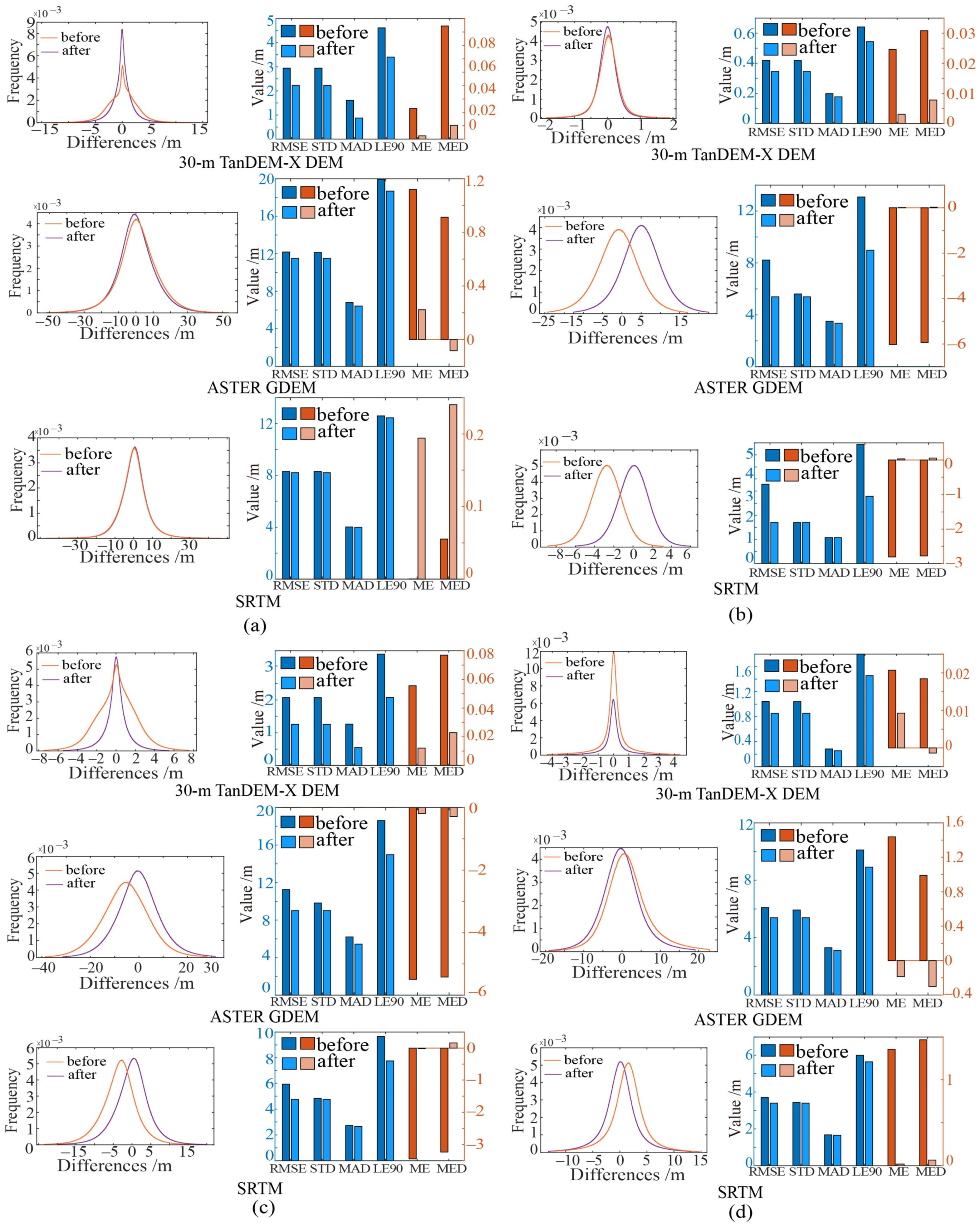
The elevation information of DEM is its important application. Therefore, the quality analysis of DEM mainly focused on its vertical quality in this study. Residuals are the height differences between the assessed DEM and the reference data at the corresponding point, which can be used to measure the vertical quality of the DEM. Mean Error (ME) (Equation (6)), Root Mean Square Error (RMSE) (Equation (7)) and Standard Deviation (STD) (Equation (8)) are the most widely used indicators for describing the characteristics of errors. In the case, where the errors follow a normal distribution, these indicators perform well [22,54,55]. However, the errors follow a non-normal distribution in most cases of DEMs [54,55]. In the case of non-normality, Median Error (MED) (Equation (9)), Median Absolute Deviation (MAD) (Equation (10)) and LE90 are more robust quality indicators [54]. For normally distributed observations, the linear error at 90% confidence level is LE90 = STD × 1.65. As height differences tend to follow a non-normal distribution, here the LE90 is directly equated to the 90th percentile of the sorted absolute differences calculated by the minimum rank method, i.e., the smallest value in the list. In other words, 90% of the data are less than or equal to that value [22,54].

$$\mathrm{ME}=\frac{{{\displaystyle \sum }}_{i=1}^N{H}_{diff}^i}{N},$$

(6)

where $H_{diff}^i$ is the height difference between the assessed DEM and the reference data at the ith point and N is the total number of errors.

$$\mathrm{RMSE}=\sqrt{\frac{{{\displaystyle \sum }}_{i=1}^N{(H_{diff}^i)}^2}{N}},$$

(7)

$$\mathrm{STD}=\sqrt{\frac{{{\displaystyle \sum }}_{i=1}^N{(H_{diff}^i-ME)}^2}{N-1}},$$

(8)

$$\mathrm{MED}=\mathrm{median}(\{H_{diff}^i\}),$$

(9)

$$\mathrm{MAD}=\mathrm{median}(\{\left|H_{diff}^i-MED\right|\}).$$

(10)

Outliers corrupt statistical accuracy measures, so the three-sigma rule was used to remove the errors satisfying Equation (11). All statistical measures presented in Section 4 are outlier-removed.

$$\left|error-ME\right|>3 \times STD.$$

(11)

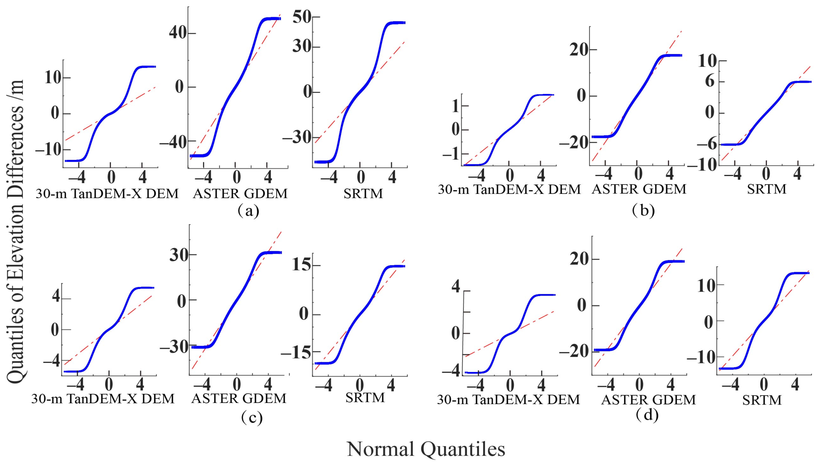
To check whether the DEM errors in this study follow a normal distribution, a normality test should be conducted. The Quantile–Quantile (Q-Q) plot can identify whether a large number of data approximates a normal distribution. It is a scatter plot with the quantiles of the residuals on the vertical axis and the quantiles of the standard normal distribution value on the horizontal axis. If the actual distribution is normal, the Q-Q plot should yield a straight line. Statistical tests can also be used to investigate whether data originate from a normal distribution, but, in the case of large datasets or outliers, these tests are often rather sensitive. Therefore, we prefer the visual method of the Q-Q plot [54].

Then, we analyzed the quality in terms of slope, aspect and land cover. We also focused on the ways in which these DEMs have been created. Since TanDEM-X DEM, ASTER GDEM and SRTM were created from the fusion of many observations, we evaluated the effect of the number of images used in the fusion process on their quality. For TanDEM-X DEM and SRTM, which were created from SAR images, the local incidence angle may impact the quality of the DEM as the geometry of the incidence angle strongly influences the quality of the reflected radar beam [15]. Because we can easily get all the original local incidence angle files used to produce the final combined SRTM in each study area, we further evaluated the effect of the local incidence angle on SRTM’s quality.

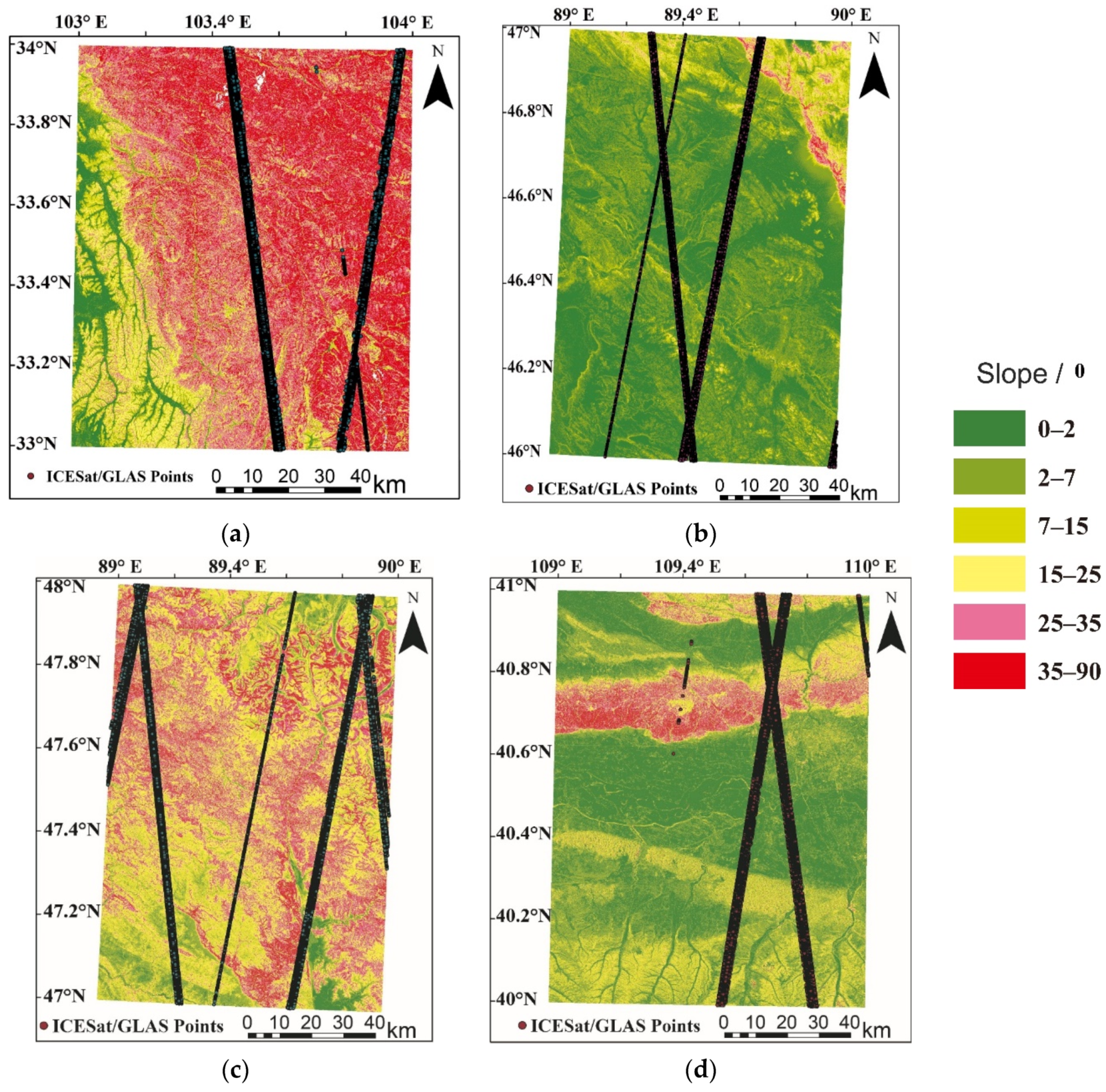
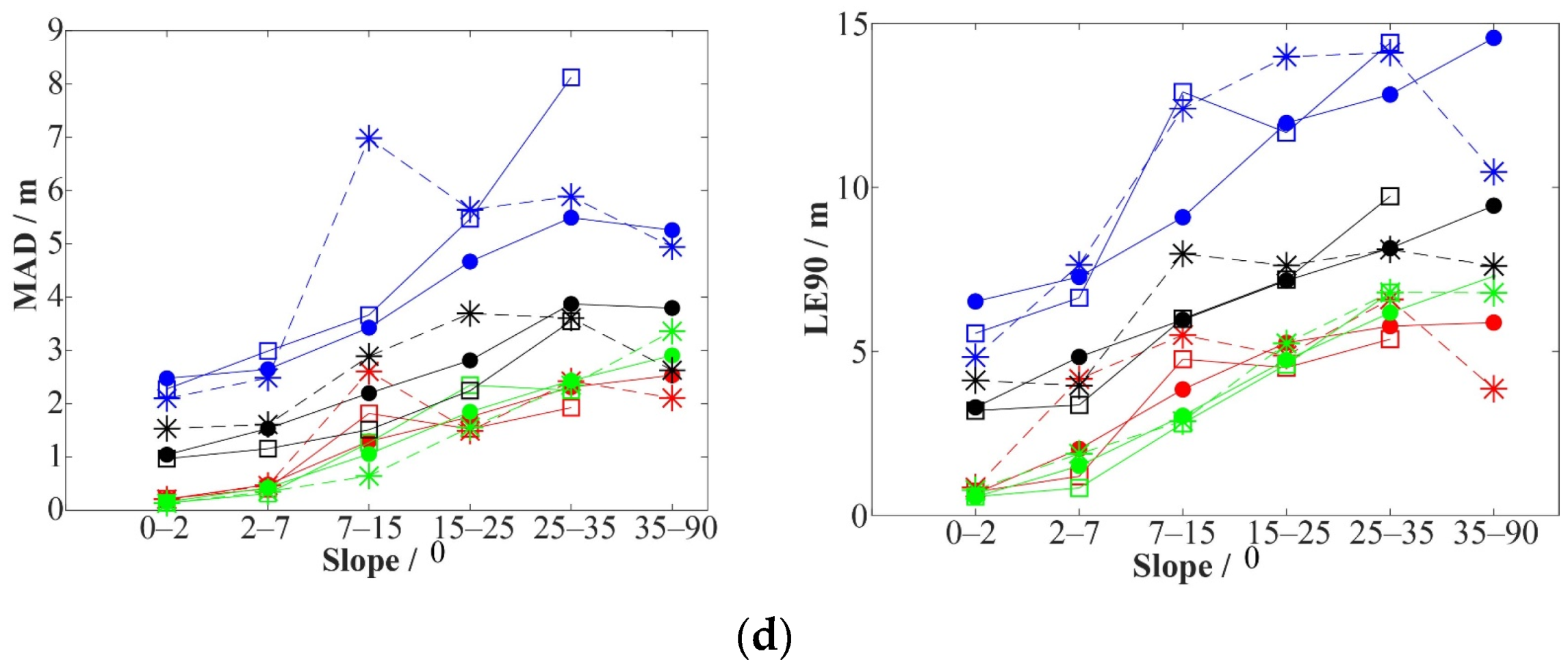
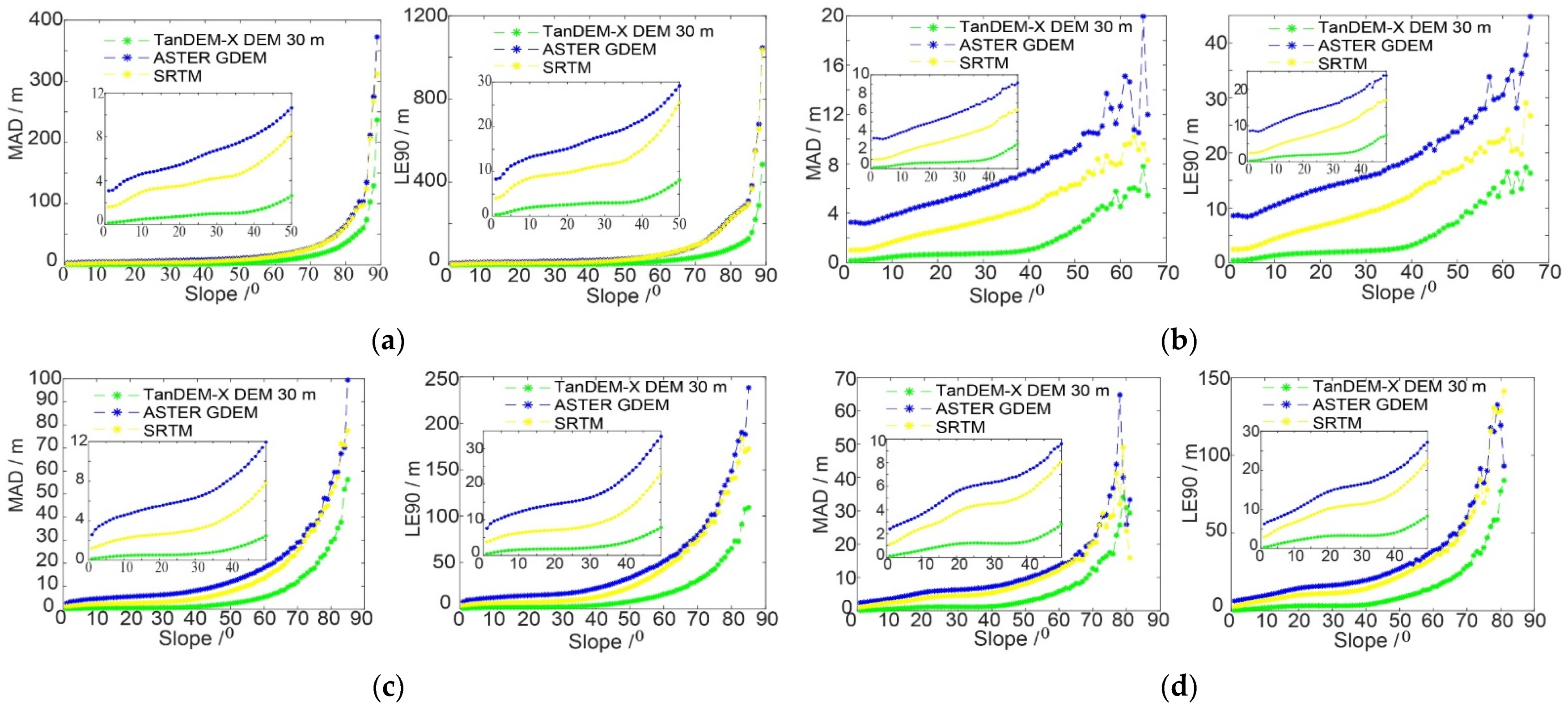
To assess the vertical quality in terms of slope, we calculated the slope of every pixel in the study areas based on the TanDEM-X DEM with a pixel size of 12 m using ArcGIS:

$${\mathrm{Slope}}_{\mathrm{radians}}= \arctan \sqrt{{\frac{dz}{dx}}^2+{\frac{dz}{dy}}^2},$$

(12)

$${\mathrm{Slope}}_{\mathrm{degrees}}={\mathrm{Slope}}_{\mathrm{radians}}\times 57.29578,$$

(13)

where $\frac{dz}{dx}$ and $\frac{dz}{dy}$ are the elevation changes in X and Y directions per unit length, respectively. When using ICESat/GLAS as the reference data, we divided the slope into six levels referring to Wang et al. [56]: 0–2° (flat), 2–7° (undulating), 7–15° (soft), 15–25° (gentle), 25–35° (steep) and more than 35° (very steep). The elevation differences were then summarized according to the binned slopes. MAD and LE90 were calculated within each slope level for assessing DEM’s quality. When using TanDEM-X DEM as the reference data, the slope bin was chosen as one degree because of the large number of differences in each bin. MAD and LE90 were also calculated.

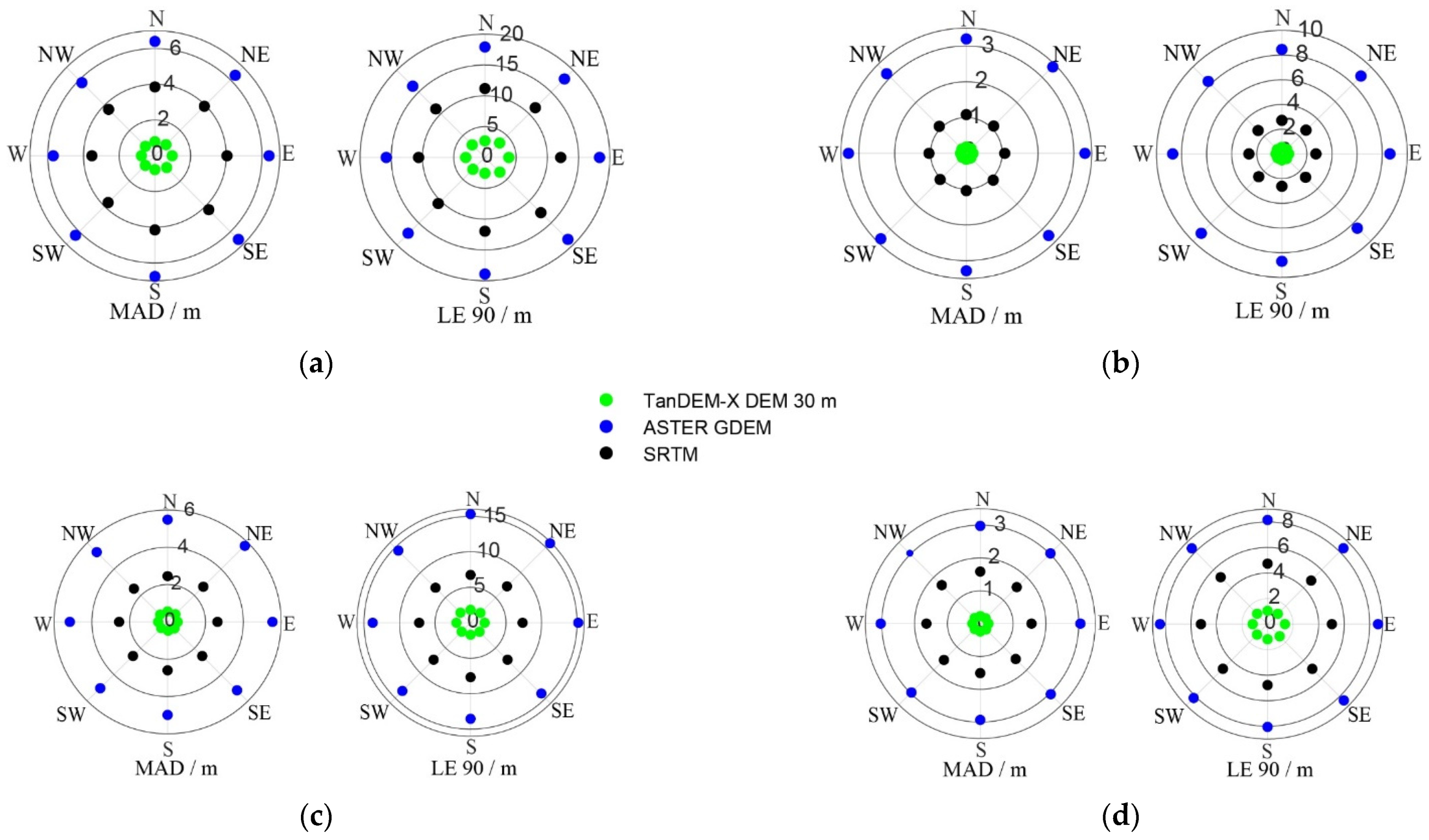
To assess the vertical quality in terms of aspect, we also calculated the aspect of every pixel in the study areas based on the TanDEM-X DEM with a pixel size of 12 m using ArcGIS, and then the aspect was divided into eight directions: N (337.5–360° and 0–22.5°), NE (22.5–67.5°), E (67.5–112.5°), SE (112.5–157.5°), S (157.5–202.5°), SW (202.5–247.5°), W (247.5–292.5°) and NW (292.5–337.5°). MAD and LE90 were calculated within each direction for assessing DEM’s quality.

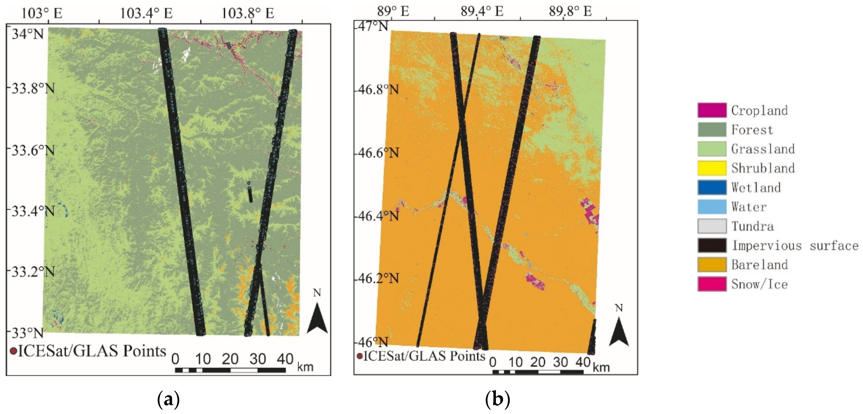
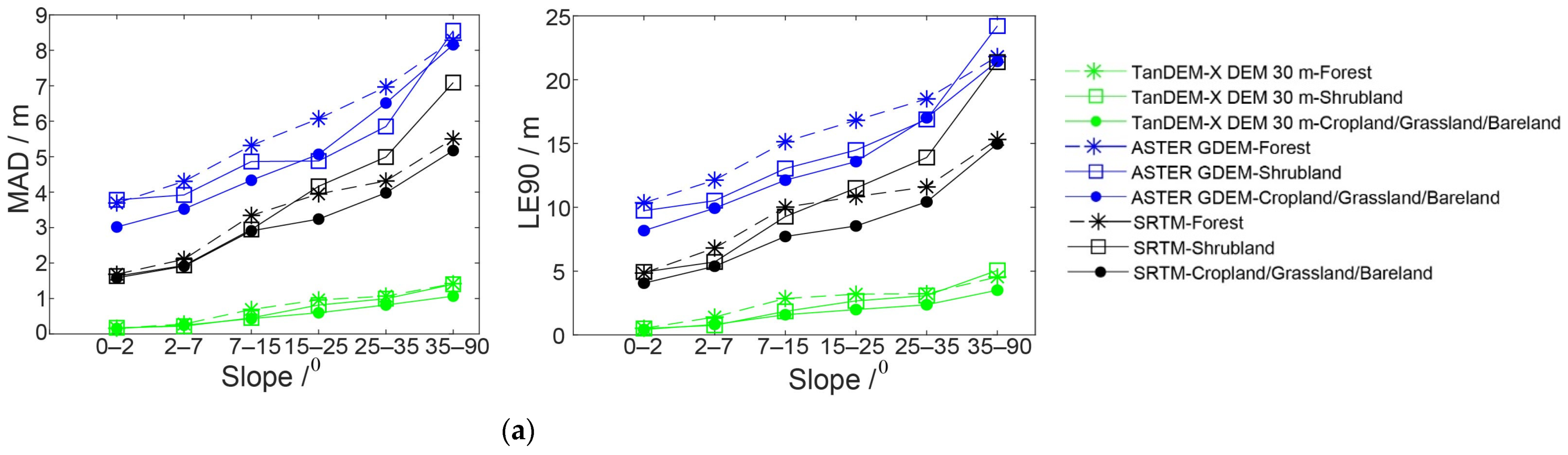
Vertical quality is also correlated to land cover. Some land cover types, such as forests, vegetation, waters, etc., will affect the elevation quality obtained by ranging and image matching. We used FROM-GLC10 land cover map with a 10-m finer resolution distributed by Gong et al. [47]. It was then bilinearly interpolated to the position of reference data after UTM projection. Ten land-cover classes were defined in the original model, but, for simplicity of analysis, three broad classes were defined referring to Varga and Bašić [13]: (1) cropland, grassland and bareland; (2) shrubland; and (3) forest. No permanent snow or ice was found in study areas. Due to their characteristics, snow, ice, water bodies and other land cover types were not considered [14]. Because of the complex topography and land cover in China, the elevation error may be affected by a combination of many factors [57]. To avoid the influence of slope, the quality of DEM under different land cover was assessed in each slope range.

When assessing the vertical quality in terms of the number of images used in the fusion process, we only took ICESat/GLAS as the reference data, avoiding the number of TanDEM-X DEM images from affecting the results of other DEMs. The number of images of each DEM was extracted at every reference point. MAD and LE90 were calculated within each quantity level.

When assessing SRTM’s quality in terms of the local incidence angle, we still only used ICESat/GLAS as the reference data. The local incidence angle was classified into three zones: (1) areas where the local incidence angle was less than the look angle, indicating a surface facing towards the radar; (2) areas where the local incidence angle was greater than the look angle, indicating a surface opposite to the radar; and (3) areas where the local incidence angle was equal to the look angle, indicating a flat surface (Figure 3). There were several local incidence angle images at each point. The zones of the point on different images maybe not the same. To avoid the joint influence and get pure results, we only analyzed the points which were in the same zone on all local incidence angle images. MAD and LE90 were calculated for each zone.

4. Results

4.1. Quality Assessment Taking ICESat/GLAS as the Reference

4.1.1. Overall Quality

Figure 4 shows the spatial distribution of elevation and ICESat/GLAS points in four study areas. Figure 5 shows the quality indicators of the four assessed DEMs using box plots. Statistics of the indicators are in Table S1.

In each study area, the changing trend of different quality indicators’ values was the same (Figure 5). That is, if the LE90 of a certain DEM is larger than that of other DEMs, then the RMSE, STD, MAD and MED of the DEM are also larger than that of other DEMs. The number of ICESat/GLAS points in Sichuan was significantly lower than that in the other three areas (Table S1). For all study areas and DEMs, except for a few cases, ME were positive. The RMSE and STD were very close. The 12- and 30-m TanDEM-X DEM showed the best quality, with MAD varying from 0.27 to 4.25 m and LE90 varying from 0.99 to 13.79 m. ASTER GDEM had the worst quality, with MAD varying from 2.81 to 8.51 m and LE90 varying from 8.68 to 23.74 m. The order of the quality of TanDEM-X DEM, ASTER GDEM and SRTM is consistent with their nominal accuracy (Table 2). We compared the quality of X-band TanDEM-X DEM and C-band SRTM with a pixel size of 30 m obtained by InSAR technology, finding that the TanDEM-X DEM had higher quality. In Sichuan and Xinjiang B, the LE90 of the 30-m TanDEM-X DEM was about 0.6 m higher than that of the 12-m TanDEM-X DEM, indicating that the quality of the 30-m TanDEM-X DEM was worse. Xinjiang A and Inner Mongolia have lower elevation, and the reference points are mainly distributed in flat areas. In these two areas, the LE90 of 12-m TanDEM-X DEM and 30-m TanDEM-X DEM were very close. Among the four areas, the quality indicators of Sichuan were the highest, which meant that the vertical quality of DEMs in Sichuan was the worst. DEMs in Xinjiang B had the second-worst quality. DEMs in Xinjiang A and Inner Mongolia had better quality.

4.1.2. Quality versus Slope

Figure 6 shows the spatial distribution of slopes in four study areas. In Sichuan, there were more than 5000 reference points distributed in areas where the slopes are >25°, accounting for about 78% of the total reference points. Only seven points were distributed in areas with slopes <2°. In Xinjiang A, there were more than 10,000 reference points distributed in areas with slopes <7°, accounting for about 92% of the total points. Fewer than 40 points were distributed in areas with slopes >25°. In Xinjiang B, there were about 75% of the points distributed in areas with slopes >15°. In Inner Mongolia, about 68% of the points were distributed in areas with slopes <7°. The slope interval where the number of pixels was less than ten was considered invalid. We used two quality indicators, MAD and LE90, to visually display the change of quality of DEMs with slopes (Figure 7). Statistics of the indicators are in Table S2.

The peaks of indicators appeared where slopes are greater than 25° (Figure 7). As the slope increased, MAD and LE90 tended to increase. The 30-m pixel size DEMs increased more drastically with increasing slopes than the 12-m pixel size TanDEM-X DEM. The MAD and LE90 of ASTER GDEM had the most dramatic increase in areas with steep slopes among the four DEMs. SRTM was the second most sensitive to slopes. When slopes were <25°, the indicators’ values of TanDEM-X DEM with a pixel size of 12 and 30 m were very close. When slopes were >25°, the values were significantly different. The MAD and LE90 of 12-m pixel size DEM were lower than those of 30-m pixel size DEM. The same DEM had different quality in four study areas within the same slope range. The values of indicators in Sichuan and Xinjiang B were larger than those in Xinjiang A and Inner Mongolia under the same slopes.

4.1.3. Quality versus Aspect

Figure S1 shows the spatial distribution of aspects in four study areas. MAD and LE90 were used to visually display the change of quality of DEMs with aspects (Figure 8). TanDEM-X DEM had a larger value in NW and a smaller value in SW in four study areas. In Xinjiang A and Inner Mongolia, where slopes are generally small, the changes of ASTER GDEM and SRTM with aspects were not obvious. In Sichuan and Xinjiang B, where have large fluctuations, MAD and LE90 were the largest near N and the smallest near S.

4.1.4. Quality versus Land Cover

Figure 9 shows the spatial distribution of land cover in four study areas. MAD and LE90 were used to visually display the change of quality of DEMs with land cover under different slopes (Figure 10). When there were less than 10 points in the conditional interval, we did not count the interval’s information. The quality of DEMs decreased with the increasing slope under the same land cover.

There was no shrubland in Sichuan, so only forest and cropland/grassland/bareland were compared. Sixty-two percent of the reference points were in the forest and 38% of the points were in the cropland/grassland/bareland. In each slope range of Sichuan, the LE90 of the other three DEMs in the forest were higher than those in the cropland/grassland/bareland, except for ASTER GDEM.

The shapes of the polylines in the forest (Figure 10a) were very close to the shapes in Figure 7a. The values in Figure 7a were basically between the values of the two land cover types in Figure 10a. However, at very steep slopes, the values in Figure 7a were higher than the maximum value of the land cover types in Figure 10a.

There were no shrubland and forest in Xinjiang A. The polylines in Figure 10b are the same as those in Figure 7b. The overall law in Xinjiang B was similar to that in Sichuan. Only 20% of the points were in the forest and 80% of the points were in the cropland/grassland/bareland, leading to the shapes of the polylines in the cropland/grassland/bareland (Figure 10c) consistent with the shapes in Figure 7c. Inner Mongolia had all three land cover types, with 3% of the points (about 300 points) in the forest, 3% of the points in the shrubland and 94% of the points in the cropland/grassland/bareland. Therefore, the shapes of the polylines in the cropland/grassland/bareland (Figure 10d) were consistent with the shapes in Figure 7d. Unlike other areas, the effect of different land covers on the quality of DEMs was not obvious in Inner Mongolia.

4.1.5. Quality versus Number of Images

Figure 11 shows the MAD and LE90 of the DEM errors in terms of the number of images used in the fusion process for TanDEM-X DEM, ASTER GDEM and SRTM in four study areas. The number of the assessed points contained under each image number is also shown in the red line. Generally, the indicators’ values decreases with an increasing number of images. For ASTER GDEM, the maximum number of images varied from 14 to 26 in four areas. For TanDEM-X DEM, the maximum number of images varied from 7 to 14. For SRTM, the maximum number of images varied from four to seven.

4.1.6. Quality versus Local Incidence Angle

Table 3. Statistical summary of SRTM error in relation to local incidence angle. Sub-swath 1: approximately 30–40° look angle. Sub-swath 2: approximately 41–48° look angle. Sub-swath 3: approximately 47–53° look angle. Sub-swath 4: approximately 52–59° look angle.

	Sichuan			Xinjiang A			Xinjiang B			Inner Mongolia
Local Incidence Angle	MAD/m	LE90/m	Points	MAD/m	LE90/m	Points	MAD/m	LE90/m	Points	MAD/m	LE90/m	Points
<look angle —facing towards the radar	4.68	13.51	368	0.21	6.68	3	3.94	11.84	975	2.36	6.61	16
>look angle —opposite to the radar	6.75	20.99	3338	1.69	5.98	77	4.15	10.25	3663	3.41	8.08	316
=look angle —flat	6.31	18.38	163	0.99	5.08	2998	1.87	7.13	438	1.42	4.68	1712

shows the statistics of SRTM in the classified three zones. The zone where the number of points was less than 20 was considered invalid, so the statistics for slopes facing towards the radar beam in Xinjiang A and Inner Mongolia were not analyzed. The indicators’ values for slopes opposite to the radar beam were the largest among the three zones. The value for slopes facing towards the radar was lower than that for the flat area in Sichuan, while the value for slopes facing towards the radar was higher than that for the flat area in Xinjiang B.

4.2. Quality Assessment Taking 12-m TanDEM-X DEM as the Reference

4.2.1. Overall Quality

Figure S2 shows a spatial distribution of original differences between the three assessed DEMs with 30-m pixel size and the reference 12-m TanDEM-X DEM before co-registration without eliminating outliers. Negative values indicate that the assessed DEM is lower than the reference DEM, while positive values indicate that the assessed DEM is higher than the reference DEM.

Table 4. Statistics of nine transformation parameters used in co-registration between the assessed DEMs and the reference DEM.

Study Area	Assessed DEM	${\mathit{T}}_{\mathit{X}}$/m	${\mathit{T}}_{\mathit{Y}}$/m	${\mathit{T}}_{\mathit{Z}}$/m	${\mathit{m}}_{\mathit{x}}$	${\mathit{m}}_{\mathit{y}}$	${\mathit{m}}_{\mathit{z}}$	${\mathit{\theta }}_{\mathit{x}}$/°	${\mathit{\theta }}_{\mathit{y}}$/°	${\mathit{\theta }}_{\mathit{z}}$/°
Sichuan	30-m TanDEM-X DEM	4.56	−1.18	−1.22	−1.86 × 10−5	−6.78 × 10−6	2.74 × 10−4	1.80 × 10−6	−1.60 × 10−6	1.07 × 10−8
	ASTER GDEM	3.76	3.59	15.85	−3.71 × 10−5	−1.01 × 10−5	−3.93 × 10−3	−3.12 × 10−5	−4.80 × 10−7	−4.94 × 10−5
	SRTM	2.10	−0.73	4.91	−1.12 × 10−5	−1.49 × 10−5	−9.63 × 10−4	−1.34 × 10−5	−6.23 × 10−7	3.22 × 10−6
Xinjiang A	30-m TanDEM-X DEM	3.50	−1.40	−0.03	9.69 × 10−6	−3.70 × 10−6	4.76 × 10−5	−7.35 × 10−8	2.79 × 10−7	−5.99 × 10−6
	ASTER GDEM	0.23	7.75	6.67	−3.66 × 10−5	2.85 × 10−5	−4.76 × 10−3	3.58 × 10−5	−5.47 × 10−5	−3.65 × 10−6
	SRTM	1.25	1.40	2.23	−2.36 × 10−5	−7.74 × 10−6	6.35 × 10−4	2.31 × 10−6	2.52 × 10−6	−1.04 × 10−5
Xinjiang B	30-m TanDEM-X DEM	4.76	−2.15	−0.09	−3.71 × 10−7	1.04 × 10−8	2.11 × 10−4	−3.02 × 10−6	3.15 × 10−6	4.55 × 10−7
	ASTER GDEM	−2.79	13.89	12.26	−1.36 × 10−5	−8.72 × 10−5	−3.58 × 10−3	3.90 × 10−5	7.29 × 10−5	−4.05 × 10−5
	SRTM	2.20	0.58	4.22	−8.31 × 10−6	−6.75 × 10−6	−5.85 × 10−4	1.26 × 10−5	1.35 × 10−5	−3.71 × 10−6
Inner Mongolia	30-m TanDEM-X DEM	3.43	−1.30	−0.15	4.73 × 10−7	−4.26 × 10−6	1.14 × 10−4	3.44 × 10−8	−1.24 × 10−7	−4.56 × 10−6
	ASTER GDEM	6.73	5.20	6.61	−1.03 × 10−5	−2.04 × 10−5	−9.28 × 10−3	−2.29 × 10−5	−6.34 × 10−5	4.42 × 10−5
	SRTM	4.56	−2.35	−4.78	−7.83 × 10−6	1.44 × 10−6	1.60 × 10−3	4.85 × 10−6	−1.59 × 10−5	1.91 × 10−5

shows the values of nine transformation parameters used in the co-registration process between the assessed DEMs and the reference DEM. Each parameter was nearly in the same order of magnitudes in different study areas for different assessed DEMs. In the vertical direction, the absolute values of $T_Z$, $m_z$ and ${\theta }_z$ of ASTER GDEM were the largest, implying the biggest vertical differences between ASTER GDEM and the reference DEM before co-registration, which was consistent with the results mentioned above.

Figure 12 shows the Q-Q plot. The vertical axis is the quantiles of elevation differences between the assessed DEMs and the reference DEM after co-registration. The horizontal axis is the normal quantiles. The red lines represent a normal distribution. All observations showed a strong deviation from the red line, indicating that the residuals had non-normal distribution even after removing the outliers.

The histograms of the differences before and after co-registration are presented in Figure 13. For each histogram, there is a corresponding bar chart showing statistical indicators of the differences. The histograms visually showed systematic errors between the assessed DEM and the reference DEM before co-registration. The x-coordinate at the peak of the histogram after co-registration was closer to zero than that before co-registration. The frequency near the peak increased after co-registration. Table S3 shows more detailed statistical results of the model-to-model comparison. The bar charts and the statistics showed decreases in the indicators’ values after co-registration.

We summarized the MAD and LE90 of the three assessed DEMs after co-registration in four study areas (Figure S3). The co-registered TanDEM-X DEM with a pixel size of 30 m had the best quality, with MAD varying from 0.18 to 0.88 m and LE90 varying from 0.54 to 3.4 m. The MAD of SRTM varied from 1.08 to 4.00 m and the LE90 varied from 2.78 to 12.45 m. ASTER GDEM had the largest values, with MAD varying from 3.10 to 6.42 m and LE90 varying from 8.92 to 18.68 m, indicating the worst quality, which was consistent with the results in Section 4.1.1. The vertical quality of the three 30-m DEMs in Sichuan was the worst. DEMs in Xinjiang A and Inner Mongolia had better quality.

4.2.2. Quality versus Slope

In Figure 6, red represents areas with higher slopes and green represents areas with lower slopes. The overall slopes of Sichuan are relatively high, followed by Xinjiang B. Inner Mongolia has a few high-slope areas. Most areas of Xinjiang A have small slopes. The spatial distribution of slopes is similar to that of the height differences (Figure S2). We set the slope bin to one degree, and the slope interval where the number of pixels was less than ten was considered invalid. MAD and LE90 were adopted to display the change of DEMs’ quality with slopes (Figure 14). In every subgraph, the indicators when the slopes were below 50° were drawn to more clearly see the changing trend in the range of 0–50° degrees.

The whole valid slope interval of Xinjiang A was 0–70°, and the maximum valid slope of the other three areas could reach to 80–90°. The relationship between the quality of DEMs and slopes was apparent. As the slope increased, the MAD and LE90 of all DEMs increased, indicating a decrease in the elevation quality. This relationship was the same for all DEMs, but the rise rates for different DEMs were different. In Xinjiang A and Inner Mongolia, where the slopes were greater than 50°, the indicators’ values had apparent fluctuations. In Sichuan and Xinjiang B, there were no such fluctuations.

In four study areas, the growth rates of MAD and LE90 suddenly increased at around 35°, but the values were still around tens of meters. The growth rates further increased at around 70°, where the values increased sharply. In the interval of 88–89° in Sichuan, the values of LE90 even reached about 1000 m. In each area, the indicators’ values of ASTER GDEM were the largest and the values of 30-m TanDEM-X DEM were the smallest, which was consistent with the results mentioned above.

4.2.3. Quality versus Aspect

Figure 15 shows the relationship between quality indicators and aspects. In each area, the assessed DEMs with 30-m pixel size had close values in eight aspects, especially in Xinjiang A and Inner Mongolia.

4.2.4. Quality versus Land Cover

Figure 16 displays the change of quality of DEMs with land cover under different slopes. The rules were similar to the results mentioned in Section 4.1.4. In addition, we found that, in each study area, the relationship between each DEM’s quality and different land cover types had the rule that the indicators’ values in very low or very high slopes were close, and the values in middle slopes were significantly different for different land cover types. In middle-slope places, the indicators’ values in forest were the largest, followed by shrubland. The values in cropland/grassland/bareland were the smallest.

5. Discussion

5.1. Overall Quality

We first discuss the results obtained with ICESat/GLAS points as the reference data. Since the accuracy of ICESat/GLAS points in mountainous regions is not high [25], many points do not meet the data preprocessing requirements in Sichuan, causing a large number of points with low quality eliminated. Positive values of ME mean that the elevation of these DEMs is generally higher than that of the reference. Part of the reason is the influence of the vegetation canopy, where short-wavelength SAR or optical satellite sensors cannot penetrate [58]. This overestimation was noted in previous studies [32,35,59,60].

TanDEM-X DEMs showed the best quality. The next-best DEM was SRTM. ASTER GDEM had the worst quality. This reflects the superiority of InSAR technology in obtaining elevation in vegetation coverage areas compared with optical technology. MAD can be used to estimate the standard deviation more resistant to outliers in the dataset. TanDEM-X DEM had the smallest MAD, meaning that it had fewer gross errors and was more robust [36]. C-band penetrates vegetation better than X-band. Therefore, the elevation obtained by C-band SAR should be closer to the surface elevation than that obtained by X-band SAR. However, the results of this study are the opposite of the theory. Part of the reason is that the fusion of multi-baseline and multi-aspect TanDEM-X DEMs improves the quality of the final TanDEM-X DEM product, which was also discussed by Liu et al. [58]. Because the acquisition time of the images used to generate the DEMs is different, we should also consider the effects of changes in vegetation and terrain over a period of time on experimental results.

In study areas with more undulating terrain, the overall quality of the 12-m TanDEM-X DEM was better than that of the 30-m TanDEM-X DEM. It means that downsampling will reduce the quality of DEM, especially in mountainous areas [35]. It also demonstrates the advantages of high-resolution DEM in describing terrain details [58]. In the other two study areas with the reference points mainly distributed in flat areas, the overall quality of the 12- and 30-m were very close. Hu et al. [35] presented similar findings.

Next, we discuss the results obtained with 12-m TanDEM-X DEM as the reference data. The fact that the residuals between DEM models had non-normal distribution was also observed in many previous studies [13,20,22]. The changes of the x-coordinate at the peak of the histogram and the frequency near the peak after co-registration reflect the reduction of systematic errors in the vertical direction [22] and the increase in the quality of the geographic location, respectively. The decreases in the indicators’ values after co-registration confirmed the conclusions of previous studies [13,23] that systematic deviations could reduce the vertical quality of DEM. These also show that the co-registration method used in this study can be used to correct the systematic errors of these DEMs. That the co-registered 30-m TanDEM-X DEM had the best quality is not unexpected because 30 m data was produced from the 12 m data using the moving-window method.

5.2. Quality versus Slope

The slope is the main factor affecting the elevation measurements [34]. The slope can cause geometric distortion in the processing of optical and SAR images, which will affect the extraction of true elevation. We first discuss the results obtained with ICESat/GLAS points as the reference data. The position where the peaks of indicators appeared indicates that the slope impacts image acquisition. As the slope increased, the quality of DEMs tended to decline, meaning the slope strongly influenced the quality of DEMs produced by InSAR or optical photogrammetry technology. The reasons for this phenomenon may be: (1) As the slope increases, the surface becomes rougher. It is challenging to measure ground elevation with optical photogrammetry and InSAR technology. (2) High-slope areas are mainly vegetation, hindering optical photogrammetry and short-wavelength SAR from measuring the ground beneath the tree canopy. (3) When the slope varies greatly, the elevation has obvious fluctuations. The value of a pixel with a size of 12 or 30 m cannot accurately represent the elevation of the land within the pixel, which can cause a large vertical error. In the flat regions, the elevation has small fluctuations, so the pixel value can basically represent the elevation of the land within the pixel. The quality of DEMs decreased with the increasing slope, which had been proven by many previous studies [61,62]. The 30-m DEMs increased more drastically with increasing slopes than the 12-m DEM, which meant that DEMs with higher resolution had a better tolerance for slope changes. When slopes were >25°, the indicators’ values of TanDEM-X DEM with a pixel size of 12 and 30 m were significantly different, which confirmed that higher-resolution DEM could better describe terrain slopes. Previous studies also made similar findings [35]. The quality of ASTER GDEM had the most dramatic decline in areas with steep slopes among the four DEMs, meaning ASTER GDEM’s vertical quality was most affected by the slope.

The same DEM had different quality in four study areas within the same slope range. The reasons may be: (1) The main land cover types in Sichuan and Xinjiang B are vegetation, while Xinjiang A and Inner Mongolia are mainly bareland. Therefore, the effects of land cover may cause this situation. (2) The slope value of the pixel is not very accurate in Sichuan and Xinjiang B with large slope changes. The pixel value may underestimate the true slope, making the classification of the errors inaccurate.

Next, we discuss the results obtained with 12-m TanDEM-X DEM as the reference data. The phenomenon that the indicators’ values had apparent fluctuations in Xinjiang A and Inner Mongolia could be related to the too few (although > 10) pixels in certain high slope bins, causing the laws in these slope bins not representative enough. In Sichuan and Xinjiang B, where had adequate pixels at high slope bins, there were no such fluctuations. In the interval of 88–89° in Sichuan, the extremely high values indicated that the quality of DEMs was seriously affected at extremely steep places. Since the 30-m TanDEM-X DEM was generated by resampling the 12-m TanDEM-X DEM, these results also show that the quality of resampling results is affected by the slope.

5.3. Quality versus Aspect

The results that the quality of DEM varies with the aspect when taking ICESat/GLAS points as the reference are similar to the previous findings [24]. The reason for the differentiation of the elevation quality with the aspect may be related to the heading of the satellite sensors in the ascending and the descending orbit [63] and the incidence angle of the radar sensor to the surface [51,57].

The strong relationship between aspects and DEM’s quality is an indicator of data misregistration [33,64]. As a result, this rule reflected that the co-registration results between DEMs were good, but high slopes and dense vegetation could influence the co-registration effects.

5.4. Quality versus Land Cover

We first discuss the results obtained with ICESat/GLAS points as the reference data. The indicators’ values of the other three DEMs in the forest were higher than those in the cropland/grassland/bareland, except for ASTER GDEM. It shows that in places with denser vegetation coverage, it is more difficult for the InSAR band to penetrate vegetation, which makes it challenging to obtain the true surface elevation. As a result, the quality of the DEMs in the forest is lower than that in the cropland/grassland/bareland. The quality of ASTER GDEM in the forest was higher than that in the cropland/grassland/bareland on a flat surface. This may be caused by ASTER GDEM’s low sensitivity to land cover, which was also mentioned by previous studies [14]. There is an interval of the acquisition time between the DEMs and the land cover map, leading to a slight change of the actual local land cover, which may also affect the results.

In Sichuan, the shapes of the polylines in the forest (Figure 10a) were very close to the shapes in Figure 7a. The reason should be that there are more reference points in the forest, which dominates the trend of all points changing with slopes in Sichuan. The reason the values in Figure 7a were higher than the maximum value of the land cover types in Figure 10a at very steep slopes is that, before calculating the indicators, we used the three-sigma rule to eliminate the outliers. For Figure 7a, we removed the outliers in each slope range. For Figure 10a, we removed the outliers in each slope range under every land cover, thus removing more outliers. Therefore, the quality at very steep slopes was improved. That the effect of different land covers on the quality of DEMs was not obvious in Inner Mongolia may be related to the few points in forest and shrubland. Only 10 s to 100 points were distributed in those two land covers under every slope range, which made the law not obvious.

Next, we discuss the results obtained with 12-m TanDEM-X DEM as the reference data. For different land cover types, the indicators’ values in very low or very high slopes were close, and the values in middle slopes were significantly different. This showed that, in flat and extremely steep places, the land cover had a small impact on vertical differences, while, in the middle slope places, the land cover had a great impact on DEM’s quality. It should be noted that the reference DEM, such as the three assessed DEMs, is also DSM, not DTM. In very steep places, the reason the quality of DEMs under different land cover was close should be that the slopes dominated the quality [34], where the impacts of land cover on DEMs’ differences became little.

5.5. Quality versus Number of Images

A larger number of images could contribute to the increasing quality of the final DEM products. For TanDEM-X DEM and SRTM, the number of images indicates the number of valid height values from different InSAR DEM acquisitions available for being fused to generate the final DEM product. In general, TanDEM-X DEM has a larger number of images than SRTM, which may be one of the reasons that TanDEM-X DEM owns a higher quality. For TanDEM-X DEM, the maximum number of images in Sichuan and Xinjiang B is larger than that in the other two study areas. This may be because Sichuan and Xinjiang B have obvious fluctuations. The previous study has similar findings that the most problematic areas are those with only one valid acquisition of TanDEM-X DEM [25]. For ASTER GDEM, the number of images represents the number of images stacked to derive the final elevation values. The previous study [35] also found that the quality of ASTER GDEM got higher with increasing stack numbers.

5.6. Quality versus Local Incidence Angle

In quality versus aspect analysis, the aspects were simply divided into eight directions, starting from true north (Section 4.1.3). By classifying the aspect into three zones according to the relationship between the local incidence angle and the look angle, the results obtained were clearer. The data opposite to the sensors have the lowest quality, which was found by the previous study on SRTM-X [15] and DEMs generated from RADARSAT stereopairs [65]. In Sichuan, the quality for slopes facing towards the radar was higher than that for the flat area, while this relationship was just the opposite in Xinjiang B. This may be partly because that the quality of ICESat/GLAS points in mountainous regions is not high [25]. This method could provide a new perspective for the quality assessment of SRTM and other DEMs whose incidence angle files are available. This also reminds us that researchers who want to generate a high-quality DEM by fusion of InSAR-derived intermediate DEMs could set low weights for places opposite to the sensors.

5.7. The Reference Data

The 30-m data were downsampled from 12-m resolution DEM using the moving-window smoothing process. Thus, when taking 12-m TanDEM-X DEM as the reference, that the 30-m TanDEM-X DEM had the best quality is not unexpected. Although the results are consistent with our expectations, the achieved quality of 30-m TanDEM-X DEM is still useful. Because these results can reflect that the downsampling process of TanDEM-X DEM is influenced by slope and landcover, and the 30-m TanDEM-X DEM agree better with the reference DEM after co-registration. It should be noted that the rather low elevation differences and unrealistic quality of 30-m TanDEM-X DEM when taking 12-m TanDEM-X DEM as the reference is because they originate from the same data source.

It might be a little confusing why we used the reference ICESat/GLAS points to assess the quality of another reference 12-m TanDEM-X DEM. This does not conflict with our objective that we want to provide some additional insights on the differences’ performance in relation to various influencing factors. Through the consistency performance between 12-m TanDEM-X DEM and ICESat points, we can observe the influence of various factors on the differences between these two data, which is exactly what this article studies. It is also helpful for us to better understand the quality obtained with 12-m TanDEM-X DEM as the reference.

5.8. Data Co-Registration

In this study, we used two kinds of reference data for DEMs’ quality assessment and comparison. In model-to-model comparison, we did co-registration between models using an improved LZD method to eliminate systematic errors. However, we did not perform co-registration when taking ICESat/GLAS points as reference data. This is because: (1) The diameter of the ICESat/GLAS spot can reach 70 m, and the distance between adjacent spots is about 172 m. By contrast, the possible systematic offsets (see Table 4) are minimal. As a result, co-registration between ICESat/GLAS points and DEMs with 12- and 30-m pixel size is not necessary. (2) The reference points we used are only ICESat/GLAS points, with no other GNSS points, causing the small number and small distribution area of reference points, which can reduce the effect of co-registration. In contrast, the reference DEM is a continuous surface, which is very suitable for co-registration.

It should be noted that the co-registration solves the systematic errors (not only planimetric systematic errors but also vertical systematic errors), so the quality of the evaluated product is not the one that the user of the product will really have. Although the quality analysis of DEMs mainly focused on their vertical quality in this study, we still need to pay attention to the systematic errors. The statistics of nine transformation parameters used in co-registration between the assessed DEMs and the reference DEM (Table 4) show the systematic errors existed in 3D direction, which the researchers need to notice to make a real evaluation of each DEM.

5.9. Limitations of Our Study

The source data of the DEMs and the land cover map were obtained at different times, so the vegetation growth and topographic changes during this period would also affect the quality assessment [35]. To minimize the potential impact changing with time, we visually inspected each obvious land cover change in Google Earth, referring to Hawker et al. [24], and confirmed that no major changes occurred. However, small changes in local places could affect the experimental results. Future research should pay attention to this situation.

When exploring the relationship between land cover and DEM’s quality, we assessed the quality under different land cover in each slope range to reduce the impact of slope on results. Future studies could also pay attention to the conjoint analysis of slope/aspect.

6. Conclusions

There are many types of global DEMs distributed by different agencies, and the elevations of different DEMs are not the same. DEM’s quality affects the results of subsequent applications. SRTM and ASTER GDEM are the most commonly used global DEMs, and TanDEM-X DEM has attracted users’ attention due to its unprecedented accuracy. TanDEM-X DEM and SRTM are InSAR products, and ASTER GDEM is a photogrammetric product. To provide some additional insights on quality assessment of 12- and 30-m resolution TanDEM-X DEMs, 30-m resolution ASTER GDEM and 30-m resolution SRTM, this study assessed differences’ performance in relation to geographical features and the ways in which DEMs have been created on selected Chinese sites, taking ICESat/GLAS points with 14-cm absolute vertical accuracy but size of 70-m diameter and 12-m resolution TanDEM-X DEM with less than 10-m absolute vertical accuracy as the reference data.

Differences’ performance shows good consistency under the assessment using two reference data. Results show that: (1) TanDEM-X DEMs have the best overall quality, followed by SRTM. ASTER GDEM has the worst quality. InSAR technology has superiority in obtaining elevation in vegetation coverage areas compared with optical technology. The fusion of multi-baseline and multi-aspect TanDEM-X DEMs improves the quality of the final TanDEM-X DEM product. The 12-m TanDEM-X DEM has significant advantages in describing terrain details. Downsampling will reduce the quality of DEM, especially in mountainous areas. (2) The slope can cause geometric distortion in the processing of optical and SAR images, which can affect the extraction of true elevation. The quality of DEMs decreases with increasing slopes. ASTER GDEM’s vertical quality is most affected by the slope. SRTM is the second most sensitive to slopes. The 12-m TanDEM-X DEM has a better tolerance for slope changes. (3) TanDEM-X DEM has a larger value in NW and a smaller value in SW. In places where slopes are generally small, the changes of ASTER GDEM and SRTM with aspects are not obvious. In places of large fluctuations, the quality of ASTER GDEM and SRTM are the lowest near N and the highest near S. After the co-registration, the assessed 30-m resolution DEMs have close quality in eight aspects, especially in areas where slopes are generally small. High slopes and dense vegetation could influence co-registration effects. (4) For TanDEM-X DEM and SRTM, the denser is the vegetation cover, the lower is the quality of DEMs because, in places with denser vegetation coverage, it is more difficult for the InSAR band to penetrate vegetation, which makes it challenging to obtain the true surface elevation. ASTER GDEM has low sensitivity to land cover. If there are more reference points in a certain land cover, the shapes of the polylines describing the change of quality with slope under that land cover are consistent with the shapes of the polylines describing the change of quality with slope under all land cover types. (5) The DEMs were created from the fusion of many observations. The quality of DEMs gets higher with the increasing number of images used in the fusion process. (6) For SRTM, which is created from SAR images, the local incidence angle can impact the quality of the DEM as the geometry of the incidence angle strongly influences the quality of the reflected radar beam. The quality in places where the slopes are opposite to the radar beam is the worst. This method could provide a new perspective for the quality assessment of SRTM and other DEMs whose incidence angle files are available. Researchers who want to generate a high-quality DEM by fusion of InSAR-derived intermediate DEMs could set low weights for places opposite to the sensors. (7) The residuals between DEM models had non-normal distribution even after co-registration. The quality of the assessed DEMs increased after co-registration. Each transformation parameter using for co-registration is nearly in the same order of magnitudes in different study areas for different assessed DEMs.

In this study, our results concluded from study areas in China are similar to the results from other areas according to previous studies. Researchers who want to know the quality of a DEM in order to use it in further applications should pay more attention to the terrain factors and land cover in their study areas and the ways in which the DEM has been created. It should be noted that the statistics in the study are influenced by tree heights, especially in hilly and mountainous places. In model-to-model comparison, the quality results of the assessed three 30-m resolution DEMs are restricted by the quality of the reference 12-m resolution TanDEM-X DEM, which is the best we could utilize at this time. Further evaluation is necessary once finer and better reference DEM becomes available. The improved LZD method applied to co-registration is one of our highlights. However, this paper does not focus on the comparison of the co-registration results between our method and other methods for these global DEMs, which is also lacking in the current research. We only describe the reasons and advantages of using the LZD method from a theoretical level. Finally, with more global DEMs distributed, increasing the types of assessed DEMs is necessary for future studies.

References

1. Hong, S.; Shen, X.; Jing, F.; Du, Z. An analysis of geomorphology characteristics of the ALTAI mountain based on DEM. Remote Sens. Land Resour. 2007, 19, 62–66. [Google Scholar]
2. Karatson, D.; Favalli, M.; Tarquini, S.; Fornaciai, A.; Woerner, G. The regular shape of stratovolcanoes: A DEM-based morphometrical approach. J. Volcanol. Geotherm. Res. 2010, 193, 171–181. [Google Scholar] [CrossRef]
3. Berthier, E.; Arnaud, Y.; Vincent, C.; Rémy, F. Biases of SRTM in high-mountain areas: Implications for the monitoring of glacier volume changes. Geophys. Res. Lett. 2006, 33. [Google Scholar] [CrossRef]
4. Colby, J.D.; Mulcahy, K.A.; Wang, Y. Modeling flooding extent from Hurricane Floyd in the coastal plains of North Carolina. Glob. Environ. Chang. Part B Environ. Hazards 2001, 2, 157–168. [Google Scholar] [CrossRef]
5. Thomas, C.D.; Cameron, A.; Green, R.E.; Bakkenes, M.; Beaumont, L.J.; Collingham, Y.C.; Erasmus, B.F.N.; de Siqueira, M.F.; Grainger, A.; Hannah, L.; et al. Extinction risk from climate change. Nature 2004, 427, 145–148. [Google Scholar] [CrossRef]
6. Smith, M.J.; Clark, C.D. Methods for the visualization of digital elevation models for landform mapping. Earth Surf. Process. Landf. 2005, 30, 885–900. [Google Scholar] [CrossRef]
7. Hawker, L.; Bates, P.; Neal, J.; Rougier, J. Perspectives on Digital Elevation Model (DEM) Simulation for Flood Modeling in the Absence of a High-Accuracy Open Access Global DEM. Front. Earth Sci. 2018, 6, 233. [Google Scholar] [CrossRef] [Green Version]
8. Wechsler, S.P. Uncertainties associated with digital elevation models for hydrologic applications: A review. Hydrol. Earth Syst. Sci. Discuss. 2007, 3, 1481–1500. [Google Scholar] [CrossRef] [Green Version]
9. Rao, Y.; Deo, R.; Nalini, J.; Pillai, A.; Muralikrishnan, S.; Dadhwal, V. Quality assessment of TanDEM-X DEMs using airborne LiDAR, photogrammetry and ICESat elevation data. ISPRS J. Photogramm. Remote Sens. 2014, 2, 187. [Google Scholar] [CrossRef] [Green Version]
10. Li, Z.; Li, P.; Ding, D.; Wang, H. Research Progress of Global High Resolution Digital Elevation Models. Geomat. Inf. Sci. Wuhan Univ. 2018, 043, 1927–1942. [Google Scholar]
11. Farr, T.G.; Rosen, P.A.; Caro, E.; Crippen, R.; Duren, R.; Hensley, S.; Kobrick, M.; Paller, M.; Rodriguez, E.; Roth, L. The Shuttle Radar Topography Mission. Rev. Geophys. 2007, 45, 361. [Google Scholar] [CrossRef] [Green Version]
12. Tachikawa, T.; Hato, M.; Kaku, M.; Iwasaki, A. Characteristics of ASTER GDEM version 2. In Proceedings of the 2011 IEEE International Geoscience and Remote Sensing Symposium, Vancouver, BC, Canada, 24–29 July 2011; pp. 3657–3660. [Google Scholar]
13. Varga, M.; Basic, T. Accuracy validation and comparison of global digital elevation models over Croatia. Int. J. Remote Sens. 2015, 36, 170–189. [Google Scholar] [CrossRef]
14. Satgé, F.; Bonnet, M.P.; Timouk, F.; Calmant, S.; Pillco, R.; Molina, J.; Lavado-Casimiro, W.; Arsen, A.; Crétaux, J.F.; Garnier, J. Accuracy assessment of SRTM v4 and ASTER GDEM v2 over the Altiplano watershed using ICESat/GLAS data. Int. J. Remote Sens. 2015, 36, 465–488. [Google Scholar] [CrossRef]
15. Kolecka, N.; Kozak, J. Assessment of the Accuracy of SRTM C- and X-Band High Mountain Elevation Data: A Case Study of the Polish Tatra Mountains. Pure Appl. Geophys. 2014, 171, 897–912. [Google Scholar] [CrossRef] [Green Version]
16. Misra, P.; Avtar, R.; Takeuchi, W. Comparison of Digital Building Height Models Extracted from AW3D, TanDEM-X, ASTER, and SRTM Digital Surface Models over Yangon City. Remote Sens. 2018, 10, 2008. [Google Scholar] [CrossRef] [Green Version]
17. Wang, L.; Chen, J.; Zhang, H.; Chen, L. Difference Analysis of SRTM C-Band DEM and ASTER GDEM for Global Land Cover Mapping. In Proceedings of the 2011 International Symposium on Image and Data Fusion, Yunnan, China, 9–11 August 2011; pp. 1–4. [Google Scholar]
18. Zink, M.; Krieger, G.; Fiedler, H.; Moreira, A. The TanDEM-X mission: Overview and status. In Proceedings of the 2007 IEEE International Geoscience and Remote Sensing Symposium, Barcelona, Spain, 23–28 July 2007; pp. 3944–3947. [Google Scholar]
19. Zink, M.; Bachmann, M.; Brautigam, B.; Fritz, T.; Hajnsek, I.; Moreira, A.; Wessel, B.; Krieger, G. TanDEM-X: The New Global DEM Takes Shape. IEEE Geosci. Remote Sens. Mag. 2014, 2, 8–23. [Google Scholar] [CrossRef]
20. Baade, J.; Schmullius, C. TanDEM-X IDEM precision and accuracy assessment based on a large assembly of differential GNSS measurements in Kruger National Park, South Africa. ISPRS J. Photogramm. Remote Sens. 2016, 119, 496–508. [Google Scholar] [CrossRef]
21. Rizzoli, P.; Martone, M.; Gonzalez, C.; Wecklich, C.; Borla Tridon, D.; Bräutigam, B.; Bachmann, M.; Schulze, D.; Fritz, T.; Huber, M.; et al. Generation and performance assessment of the global TanDEM-X digital elevation model. ISPRS J. Photogramm. Remote Sens. 2017, 132, 119–139. [Google Scholar] [CrossRef] [Green Version]
22. Wessel, B.; Huber, M.; Wohlfart, C.; Marschalk, U.; Kosmann, D.; Roth, A. Accuracy assessment of the global TanDEM-X Digital Elevation Model with GPS data—ScienceDirect. ISPRS J. Photogramm. Remote Sens. 2018, 139, 171–182. [Google Scholar] [CrossRef]
23. Vassilaki, D.; Stamos, A. The 0.4 arc-sec TanDEM-X intermediate DEM with respect to the SRTM and aster global DEMS. ISPRS Int. Arch. Photogramm. Remote Sens. Spat. Inf. Sci. 2015, XL–3/W2, 253–259. [Google Scholar] [CrossRef] [Green Version]
24. Hawker, L.; Neal, J.; Bates, P. Accuracy assessment of the TanDEM-X 90 Digital Elevation Model for selected floodplain sites. Remote Sens. Environ. 2019, 232, 111319. [Google Scholar] [CrossRef]
25. Gdulová, K.; Mareová, J.; Moudr, V. Accuracy assessment of the global TanDEM-X digital elevation model in a mountain environment. Remote Sens. Environ. 2020, 241, 111724. [Google Scholar] [CrossRef]
26. Pipaud, I.; Loibl, D.; Lehmkuhl, F. Evaluation of TanDEM-X elevation data for geomorphological mapping and interpretation in high mountain environments—A case study from SE Tibet, China. Geomorphology 2015, 246, 232–254. [Google Scholar] [CrossRef]
27. Pandey, P.; Manickam, S.; Bhattacharya, A.; Ramanathan, A.L.; Venkataraman, G. Qualitative and quantitative assessment of TanDEM-X DEM over western Himalayan glaciated terrain. Geocarto Int. 2017, 32, 442–454. [Google Scholar] [CrossRef]
28. Keys, L.; Baade, J. Uncertainty in Catchment Delineations as a Result of Digital Elevation Model Choice. Hydrology 2019, 6, 13. [Google Scholar] [CrossRef] [Green Version]
29. Kramm, T.; Hoffmeister, D. A Relief Dependent Evaluation of Digital Elevation Models on Different Scales for Northern Chile. Int. J. Geo Inf. 2019, 8, 430. [Google Scholar] [CrossRef] [Green Version]
30. Podgórski, J.; Kinnard, C.; Pętlicki, M.; Urrutia, R. Performance Assessment of TanDEM-X DEM for Mountain Glacier Elevation Change Detection. Remote Sens. 2019, 11, 187. [Google Scholar] [CrossRef] [Green Version]
31. Kumar, A.; Negi, H.S.; Kumar, K.; Shekhar, C. Accuracy Validation and Bias Assessment of Various Multi-Sensor Open Source DEMs in Part of the Karakoram Region. Remote Sens. Lett. 2020, 11, 893–902. [Google Scholar] [CrossRef]
32. Uuemaa, E.; Ahi, S.; Montibeller, B.; Muru, M.; Kmoch, A. Vertical Accuracy of Freely Available Global Digital Elevation Models (ASTER, AW3D30, MERIT, TanDEM-X., SRTM, and NASADEM). Remote Sens. 2020, 12, 3482. [Google Scholar] [CrossRef]
33. Grohmann, C.H. Evaluation of TanDEM-X DEMs on selected Brazilian sites: Comparison with SRTM, ASTER GDEM and ALOS AW3D30. Remote Sens. Environ. 2018, 212, 121–133. [Google Scholar] [CrossRef] [Green Version]
34. Zhang, Q.; Yang, Q.; Wang, C. SRTM Error Distribution and its Associations with Landscapes across China. Photogramm. Eng. Remote Sens. J. Am. Soc. Photogramm. 2016, 82, 135–148. [Google Scholar] [CrossRef]
35. Hu, Z.; Peng, J.; Hou, Y.; Shan, J. Evaluation of Recently Released Open Global Digital Elevation Models of Hubei, China. Remote Sens. 2017, 9, 262. [Google Scholar] [CrossRef] [Green Version]
36. Guan, L.; Pan, H.; Zou, S.; Hu, J.; Zhou, P. The impact of horizontal errors on the accuracy of freely available Digital Elevation Models (DEMs). Int. J. Remote Sens. 2020, 41, 7367–7383. [Google Scholar] [CrossRef]
37. Schutz, B.E.; Zwally, H.J.; Shuman, C.A.; Hancock, D.; Dimarzio, J.P. Overview of the ICESat Mission. Geophys. Res. Lett. 2005, 32, 97–116. [Google Scholar] [CrossRef] [Green Version]
38. Rosenholm, D.; Torlegard, K. 3-dimensional absolute orientation of stereo models using digital elevation models. Photogramm. Eng. Remote Sens. 1988, 54, 1385–1389. [Google Scholar]
39. Gruber, A.; Wessel, B.; Martone, M.; Roth, A. The TanDEM-X DEM Mosaicking: Fusion of Multiple Acquisitions Using InSAR Quality Parameters. IEEE J. Sel. Top. Appl. Earth Obs. Remote Sens. 2016, 9, 1047–1057. [Google Scholar] [CrossRef]
40. Hajnsek, I.; Krieger, G.; Werner, M.; Younis, M.; Zink, M.; Moreira, A.; Fiedler, H. TanDEM-X: A Satellite Formation for High-Resolution SAR Interferometry. IEEE Trans. Geosci. Remote Sens. 2007, 45, 3317–3341. [Google Scholar]
41. Krieger, G.; Zink, M.; Bachmann, M.; Brutigam, B.; Moreira, A. TANDEM-X: A radar interferometer with two formation flying satellites. Acta Astronaut. 2013, 89, 83–98. [Google Scholar] [CrossRef] [Green Version]
42. Martone, M.; Braeutigam, B.; Rizzoli, P.; Gonzalez, C.; Bachmann, M.; Krieger, G. Coherence evaluation of TanDEM-X interferometric data. ISPRS J. Photogramm. Remote Sens. 2012, 73, 21–29. [Google Scholar] [CrossRef] [Green Version]
43. Bräutigam, B.; Zink, M.; Hajnsek, I.; Krieger, G. The TanDEM-X Mission: Earth Observation in 3D. In Proceedings of the Geomorphometry, Nangjing, China, 16–20 October 2013; pp. 1–4. [Google Scholar]
44. Wecklich, C.; Gonzalez, C.; Rizzoli, P. TANDEM-X height performance and data coverage. In Proceedings of the 2017 IEEE International Geoscience and Remote Sensing Symposium (IGARSS), Fort Worth, TX, USA, 23–28 July 2017; pp. 4088–4091. [Google Scholar]
45. Yamaguchi, Y.; Kahle, A.B.; Tsu, H.; Kawakami, T.; Pniel, M. Overview of Advanced Spaceborne Thermal Emission and Reflection Radiometer (ASTER). IEEE Trans. Geosci. Remote Sens. 2002, 36, 1062–1071. [Google Scholar] [CrossRef] [Green Version]
46. Abshire, J.; Sun, X.; Riris, H.; Sirota, J.; McGarry, J.; Palm, S.; Yi, D.; Liiva, P. Geoscience Laser Altimeter System (GLAS) on the ICESat Mission: On-orbit measurement performance. Geophys. Res. Lett. 2005, 32, 21–22. [Google Scholar] [CrossRef] [Green Version]
47. Gong, P.; Liu, H.; Zhang, M.; Li, C.; Wang, J.; Huang, H.; Clinton, N.; Ji, L.; Li, W.; Bai, Y.; et al. Stable classification with limited sample: Transferring a 30-m resolution sample set collected in 2015 to mapping 10-m resolution global land cover in 2017. Sci. Bull. 2019, 64, 370–373. [Google Scholar] [CrossRef] [Green Version]
48. Guan, L.; Chen, S.; Zou, S.; Wu, W. Comparative Analysis of Several Freely Available DEM Datasets. Geomat. Spat. Inf. Technol. 2020, 43, 21–23, (In Chinese with English Abstract). [Google Scholar]
49. Bhang, K.J.; Schwartz, F.W.; Braun, A. Verification of the Vertical Error in C-Band SRTM DEM Using ICESat and Landsat-7, Otter Tail County, MN. IEEE Trans. Geosci. Remote Sens. 2007, 45, 36–44. [Google Scholar] [CrossRef]
50. Wang, X.; Gong, P.; Zhao, Y.; Xu, Y.; Cheng, X.; Niu, Z.; Luo, Z.; Huang, H.; Sun, F.; Li, X. Water-level changes in China’s large lakes determined from ICESat/GLAS data. Remote Sens. Environ. 2013, 132, 131–144. [Google Scholar] [CrossRef]
51. Wan, J.; Liao, J.; Xu, T.; Shen, G. Accuracy evaluation of SRTM data based on ICESat /GLAS altimeter data: A case study in the Tibetan Plateau. Remote Sens. Land Resour. 2015, 27, 100–105. [Google Scholar]
52. Wenjiao, W.; Shifang, Z.; Shangmin, Z. Analysis and Comparison of SRTM1 DEM and ASTER GDEM V2 Data. J. Geo Inf. Sci. 2017, 19, 1108–1115. [Google Scholar]
53. Balzter, H.; Baade, J.; Rogers, K. Validation of the TanDEM-X Intermediate Digital Elevation Model With Airborne LiDAR and Differential GNSS in Kruger National Park. IEEE Geosci. Remote Sens. Lett. 2016, 13, 277–281. [Google Scholar] [CrossRef] [Green Version]
54. Hoehle, J.; Hoehle, M. Accuracy assessment of digital elevation models by means of robust statistical methods. ISPRS J. Photogramm. Remote Sens. 2009, 64, 398–406. [Google Scholar] [CrossRef] [Green Version]
55. Müller, J.; Gärtner-Roer, I.; Thee, P.; Ginzler, C. Accuracy assessment of airborne photogrammetrically derived high-resolution digital elevation models in a high mountain environment. ISPRS J. Photogramm. Remote Sens. 2014, 98, 58–69. [Google Scholar] [CrossRef]
56. Hong, W.; Jun, W. Preliminary study on specification of basic terrain-unit dataset. Sci. Surv. Mapp. 2004, 29, 22–25. [Google Scholar]
57. Zhiyuan, G.; Yuanli, X.; Ninglian, W.; Guangxin, J.; Peng, Z. Response of three global DEM Data accuracy to different terrain factors in Qinghai-Tibet Plateau. Bull. Soil Water Conserv. 2019, 39, 190–197. [Google Scholar]
58. Liu, Z.; Zhu, J.; Fu, H.; Zhou, C.; Zuo, T. Evaluation of the Vertical Accuracy of Open Global DEMs over Steep Terrain Regions Using ICESat Data: A Case Study over Hunan Province, China. Sensors 2020, 20, 4865. [Google Scholar] [CrossRef]
59. Athmania, D.; Achour, H. External Validation of the ASTER GDEM2, GMTED2010 and CGIAR-CSI- SRTM v4.1 Free Access Digital Elevation Models (DEMs) in Tunisia and Algeria. Remote Sens. 2014, 6, 4600–4620. [Google Scholar] [CrossRef] [Green Version]
60. Mukherjee, S.; Joshi, P.K.; Mukherjee, S.; Ghosh, A.; Garg, R.D.; Mukhopadhyay, A. Evaluation of vertical accuracy of open source Digital Elevation Model (DEM)—ScienceDirect. Int. J. Appl. Earth Obs. Geoinf. 2013, 21, 205–217. [Google Scholar] [CrossRef]
61. Bolstad, P.V.; Stowe, T. Evaluation of DEM accuracy. Elevation, slope, and aspect. Photogramm. Eng. Remote Sens. 1994, 60, 1327–1332. [Google Scholar]
62. Zhou, Q.; Liu, X. Analysis of errors of derived slope and aspect related to DEM data properties. Comput. Geosci. 2004, 30, 369–378. [Google Scholar] [CrossRef]
63. Shortridge, A.; Messina, J. Spatial structure and landscape associations of SRTM error. Remote Sens. Environ. 2011, 115, 1576–1587. [Google Scholar] [CrossRef]
64. Chen, C.; Yang, S.; Li, Y. Accuracy Assessment and Correction of SRTM DEM Using ICESat/GLAS Data under Data Coregistration. Remote Sens. 2020, 12, 3435. [Google Scholar] [CrossRef]
65. Toutin, T. Impact of terrain slope and aspect on radargrammetric DEM accuracy. ISPRS J. Photogramm. Remote Sens. 2002, 57, 228–240. [Google Scholar] [CrossRef]
Figure 1. The location distribution of four study areas in China and images of their topography (generated from 12-m TanDEM-X DEM).
Remotesensing 13 01304 g001
Figure 2. The general workflow of this study.
Remotesensing 13 01304 g002
Figure 3. The geometry of the incidence angle.
Remotesensing 13 01304 g003
Figure 4. The spatial distribution of elevation in four study areas and the distribution of ICESat/GLAS points: (a) Sichuan; (b) Xinjiang A; (c) Xinjiang B; and (d) Inner Mongolia. There are 8804, 13,657, 18,669 and 13,770 reference points in the four study areas before data preprocessing, respectively.
Remotesensing 13 01304 g004
Figure 5. Quality indicators of the four assessed DEMs in study areas: (a) Sichuan; (b) Xinjiang A; (c) Xinjiang B; and (d) Inner Mongolia.
Remotesensing 13 01304 g005
Figure 6. The spatial distribution of slopes in four study areas and the distribution of ICESat/GLAS points: (a) Sichuan; (b) Xinjiang A; (c) Xinjiang B; and (d) Inner Mongolia.
Remotesensing 13 01304 g006
Figure 7. The relationship between quality indicators ((left) MAD and (right) LE90) and slopes in four study areas: (a) Sichuan; (b) Xinjiang A; (c) Xinjiang B; and (d) Inner Mongolia.
Remotesensing 13 01304 g007
Figure 8. The relationship between quality indicators ((left) MAD and (right) LE90) and aspects in four study areas: (a) Sichuan; (b) Xinjiang A; (c) Xinjiang B; and (d) Inner Mongolia.
Remotesensing 13 01304 g008
Figure 9. The spatial distribution of land cover in four study areas and the distribution of ICESat/GLAS points: (a) Sichuan; (b) Xinjiang A; (c) Xinjiang B; and (d) Inner Mongolia.
Remotesensing 13 01304 g009aRemotesensing 13 01304 g009b
Figure 10. The relationship between quality indicators ((left) MAD and (right) LE90) and land cover in four study areas: (a) Sichuan; (b) Xinjiang A; (c) Xinjiang B; and (d) Inner Mongolia.
Remotesensing 13 01304 g010aRemotesensing 13 01304 g010b
Figure 11. MAD and LE90 of the DEM errors versus the number of images used in the fusion process for TanDEM-X DEM, ASTER GDEM and SRTM in four study areas: (a) Sichuan; (b) Xinjiang A; (c) Xinjiang B; and (d) Inner Mongolia. The number of points contained under each image number is also shown as a separate curve.
Remotesensing 13 01304 g011
Figure 12. Q-Q plot. The vertical axis is the quantiles of elevation differences between the assessed DEMs and the reference DEM after co-registration in: (a) Sichuan; (b) Xinjiang A; (c) Xinjiang B; and (d) Inner Mongolia. The horizontal axis is the normal quantiles. The blue scatters are the observations. The red lines represent a normal distribution.
Remotesensing 13 01304 g012
Figure 13. Histograms of the elevation differences between models before and after co-registration, and corresponding bar charts showing statistical indicators in: (a) Sichuan; (b) Xinjiang A; (c) Xinjiang B; and (d) Inner Mongolia.
Remotesensing 13 01304 g013
Figure 14. The relationship between quality indicators ((left) MAD and (right) LE90) and slopes in: (a) Sichuan; (b) Xinjiang A; (c) Xinjiang B; and (d) Inner Mongolia.
Remotesensing 13 01304 g014
Figure 15. The relationship between quality indicators ((left) MAD and (right) LE90) and aspects in four study areas: (a) Sichuan; (b) Xinjiang A; (c) Xinjiang B; and (d) Inner Mongolia.
Remotesensing 13 01304 g015
Figure 16. The relationship between quality indicators ((left) MAD and (right) LE90) and land cover in four study areas: (a) Sichuan; (b) Xinjiang A; (c) Xinjiang B; and (d) Inner Mongolia.
Remotesensing 13 01304 g016aRemotesensing 13 01304 g016b