Article

Lithology Discrimination Using Sentinel-1 Dual-Pol Data and SRTM Data

College of Geo-exploration Science and Technology, Jilin University, Changchun 130026, China
*
Author to whom correspondence should be addressed.
Remote Sens. 2021, 13(7), 1280; https://doi.org/10.3390/rs13071280
Submission received: 9 March 2021 / Revised: 21 March 2021 / Accepted: 24 March 2021 / Published: 27 March 2021

Abstract

:
Compared to various optical remote sensing data, studies on the performance of dual-pol Synthetic aperture radar (SAR) on lithology discrimination are scarce. This study aimed at using Sentinel-1 data to distinguish dolomite, andesite, limestone, sandstone, and granite rock types. The backscatter coefficients VV and VH, the ratio VV–VH; the decomposition parameters Entropy, Anisotropy, and Alpha were firstly derived and the Kruskal–Wallis rank sum test was then applied to these polarimetric derived matrices to assess the significance of statistical differences among different rocks. Further, the corresponding gray-level co-occurrence matrices (GLCM) features were calculated. To reduce the redundancy and data dimension, the principal component analysis (PCA) was carried out on the GLCM features. Due to the limited rock samples, before the lithology discrimination, the input variables were selected. Several classifiers were then used for lithology discrimination. The discrimination models were evaluated by overall accuracy, confusion matrices, and the area under the curve-receiver operating characteristics (AUC-ROC). Results show that (1) the statistical differences of the polarimetric derived matrices (backscatter coefficients, ratio, and decomposition parameters) among different rocks was insignificant; (2) texture information derived from Sentinel-1 had great potential for lithology discrimination; (3) partial least square discrimination analysis (PLSDA) had the highest overall accuracy (0.444) among the classification models; (4) though the overall accuracy is unsatisfactory, according to the AUC-ROC and confusion matrices, the predictive ability of PLSDA model for limestone is high with an AUC value of 0.8017, followed by dolomite with an AUC value of 0.7204. From the results, we suggest that the dual-pol Sentinel-1 data are able to correctly distinguish specific rocks and has the potential to capture the variation of different rocks.

Graphical Abstract

1. Introduction

Lithology identification is essential for geological investigation and mineral resource exploration. Accurate information on lithology provides a profound basis to trace the process of planetary formation [1]. The traditional way to discriminate lithology is usually based on field investigation and laboratory experiments, which is expensive and time-consuming. Remote sensing technology makes it possible to identify lithology on a large scale efficiently and timely, especially when the terrain is rugged and the topography is complex [2,3].
The performance of remote sensing on lithology classification has been widely explored and most of the studies concentrated on the use of spectral features. The spectra of rocks and minerals usually have special absorption features and these features can be due to various physical and chemical properties like the size of grains in rock, the composition, texture, element content, etc. [4,5]. Lyon [6] found that the depth of the spectra could be affected by the grain size in igneous rock and the spectral features caused by Si-O bond vibration were influenced by the silica content. Kahle [7] utilized the multispectral thermal infrared (TIR) data obtained by airborne NASA’s (National Aeronautics and Space Administration) Bendix scanner to separate silicic igneous rock, Paleozoic quartzite, and carbonate rock. TIR spectra were further utilized for sedimentary rocks discriminant by Bihong and Xiaowei [8]; they used the data from Airborne Thermal Infrared Multispectral Scanner data and corresponding laboratory analysis to distinguish sandstones, siltstones, and carbonate rocks. Several other airborne TIR remote sensing instruments also manifest the usefulness of TIR in lithological and mineralogical mapping [9,10]. These airborne measurements, compared to satellite instruments, are only available at a few places and have a higher operational cost. As an alternative and comparable way, satellite remote sensing is more widely used due to the low cost and large-scale observations.
Various optical satellite data were applied and deployed fruitful results in lithology mapping. The spectral ratio of selected bands [11] and diagnostic mineralogical indices [12,13] extracted from ASTER was proposed for lithology mapping, according to the TIR spectral properties of typical rocks. The spectral region from visible and near-infrared (VNIR) to shortwave infrared (SWIR) also contributed a lot to lithology mapping and mineral exploration [14,15,16,17]. The efficiency of different band combinations and false-color composite for lithology differentiation using Landsat series data were studied by [18,19,20]. Ge [21] assessed the potential of Sentinel-2A imagery for lithology mapping and concluded that Sentinel-2A can yield higher accuracy than ASTER and Landsat 8 imagery because of the high spectral resolution in VNIR and SWIR range. In addition to the broadband spectral imagery, hyperspectral data like Earth Observing-1 Hyperion data can offer detailed spectral information which enables the subtle difference in spectrum among rocks that can be detected, though satellite-based hyperspectral data often contain poor spatial resolution [22,23]. In addition to spectral information, several researchers also attempted to integrate texture (spatial) features and Digital Elevation Model (DEM) [21,24,25] to enhance the accuracy of lithology mapping.
Normally, lithology mapping using satellite-based imagery requires a cloud-free environment, high outcrop density, and less vegetation cover. Moreover, unlike spectral imagery which can only provide information about the topmost part of the surface, synthetic aperture radar (SAR) technique can penetrate through the cloud and show high sensitivity to terrain surface physical properties. The amount of the backscatter SAR waves can be affected by the surface roughness and dielectric constant [26]. The dielectric constant is strongly influenced by the moisture content and conductivity. As for different rock types, the corresponding porosity, which can contain water, and the conductible metal content can result in various dielectric constants. Surface roughness can be influenced by the grain size of the rock and the general topography. Meanwhile, SAR images are also rich in textural characteristics [27]. Thus, SAR data show great potential in structural, lithology mapping, and geological investigation [28,29,30].
Recently, full-polarization SAR data have already been employed in lithology mapping. Xie et al. [31] found that the full-polarization Advanced Land Observation Satellite (ALOS) data can result in good lithology classification using Cloude-Pottier decomposition and support vector machine (SVM). Yuan et al. [32] evaluated the supplementary effect of radar on optical data in lithology identification by superimposing RADARSAT-2 on ASTER and found that full-polarization SAR images can effectively boost up the accuracy of lithology classification. Ghafouri et al. [33] used TerraSAR-X SAR data to measure the surface roughness of geological rocks, and then improve the description of geological rock surface. Radford et al. [34] made an accurate classification of geology in an environment with thick vegetation, limited outcrop, rugged terrain using airborne Terrain Observation with Progressive Scans SAR (TopSAR), coupled with geophysical (gravity and magnetics) data. Wang et al. [35] proposed a novel lithology classification method based on dual-frequency Pol-SAR data and a deep learning method. They integrated superpixels produced by stacked sparse autoencoder and contextual information of the neighborhood to increase the class separability of lithology. The above literature indicates that SAR has advantages for lithology mapping. However, most of the studies used high-cost commercial data, and the SAR data are often full-polarization data (HH, HV, VV, VH). Sentinel-1 as a good trade-off between cost and spatial-temporal resolution offers dual polarization (VV and VH) data. The potential of dual-pol Sentinel-1 data for lithology mapping or discrimination still needs further study.
Among the discrimination or classification methods, pixel-based methods are a common technique used for mapping or classifying lithological units [36]. The pixel-based classifiers consist of parametric (maximum likelihood) and non-parametric (SVM, neural networks, and tree-based) classifiers. Contrary to the parametric classifiers, the normally distributed data are not required by the non-parametric classifiers. Due to the fact that remote sensing data cannot provide data with normal distribution in most cases, the non-parametric classifiers are more preferred [22]. Partial least square discriminant analysis (PLSDA), as a non-parametric machine learning tool, combines the PLS regression and classification techniques. Unlike the neural network classifiers, partial least square (PLS)can still show robust and effective results with a small sample size [22,37]. Whereas PLSDA has shown great potential in many fields like bioinformatics, agriculture, and chemometrics, the usage of PLSDA in lithology discrimination is rarely mentioned.

2. Study Area and Materials

2.1. Study Area and Field Samples

The study area is located in Huludao, a southwest coastal city with many hills in Liaoning Province, China. This region is on the West Block of North China Craton, which is one of the oldest Archean cratons in the world, and experienced widespread tectono-thermal activity since the late Mesozoic [38,39]. The various lithological rock outcrops with different characteristics can be found in this area.
Fifty-four rock samples were randomly distributed in Huludao (Figure 1). GPS positions and physical properties like color, grain size, and texture were recorded. In general, the sample was grouped into five kinds of rock as follows: andesite (n = 17), dolomite (n = 7), granite (n = 9), limestone (n = 15), and sandstone (n = 6). To reduce the effect from the dense vegetation cover with plenty of forest and cropland, most of the samples were located in open and unobstructed places.

2.2. Sentinel-1 Products and Elevation Data
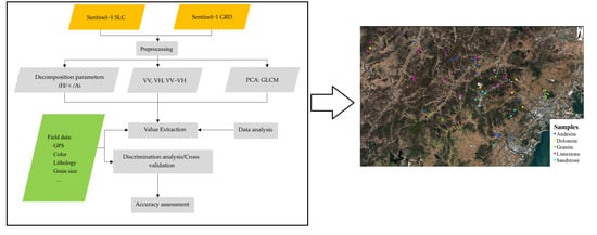
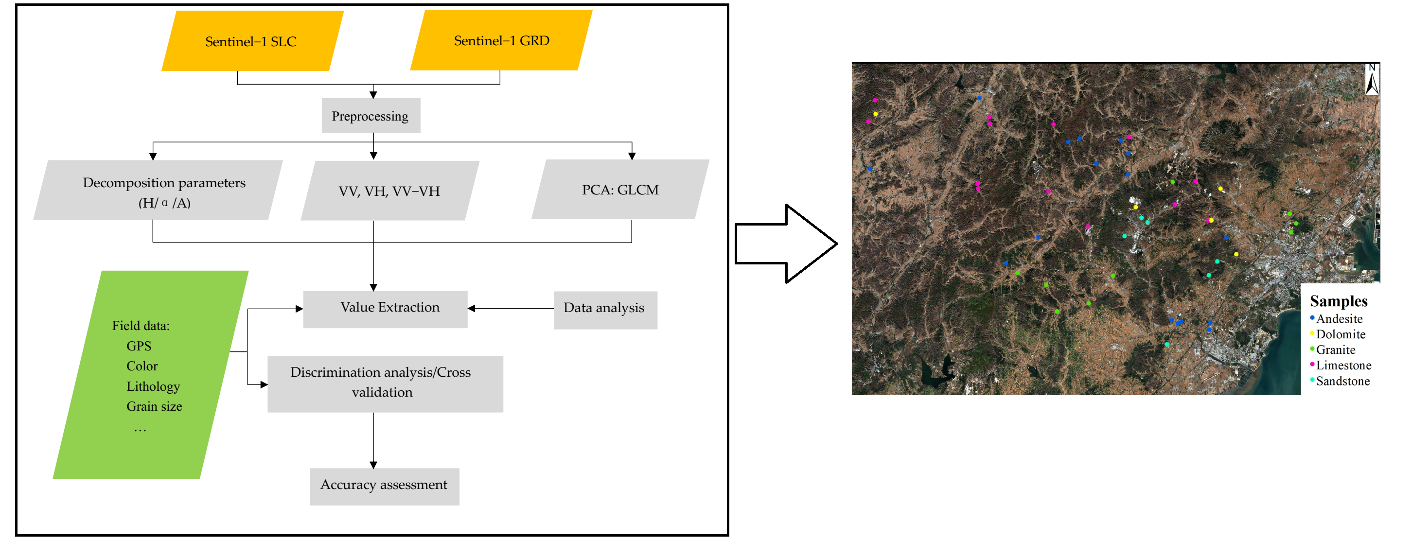
The Sentinel-1 mission is part of the Copernicus Programme developed by the European Agency, containing Sentinel-1A and Sentinel-1B constellations. Level-1 single-look complex (SLC) and Ground range detected (GRD) Sentinel-1 products providing dual-polarization (VV and VH) data, in Interferometric Wide Swath (IW) mode were utilized in this study. SLC products consist of focused SAR data geo-referenced using orbit and attitude data from satellite and provide in zero-Doppler slant-range geometry. GRD products consist of focused SAR data that have been detected, multi-looked, and projected to ground range using the WGS-84 Earth ellipsoid model. To reduce the effect of vegetation and snow cover, data acquired on 8 October 2020 were selected.
Due to the close relationship between topography, tectonic process, and lithology [40], elevation data were also involved in this study. SRTM (The Shuttle Radar Topography Mission) 1 Arc-Second Global elevation data generated from C-band Spaceborne Imaging Radar and the X-band SAR instrument onboard the space shuttle were used here.

3. Methodology

The methodology (Figure 2) mainly consists of 4 parts: (1) preprocessing of Sentinel-1 GRD and SLC data and the extraction of corresponding polarimetric parameters of samples; (2) statistical analysis of polarimetric parameters; (3) discriminant analysis on the sample and cross-validation; (4) accuracy assessment.

3.1. Sentinel-1 Preprocessing

The preprocessing for Sentinel-GRD data was similar as described in [41]. As such, the orbit information was firstly updated to obtain the precise position of the satellite. Radiometric calibration was then done to convert the digital value to radiometrically calibrated SAR backscatter. The images were cropped to reduce image size and processing time. The speckle noise generated from the interference of waves from elementary scatterers was filtered by the refined Lee filter, as it can preserve point target and texture information [42]. Range Doppler terrain correction compensates the geometry distortion caused by side-looking working mode and topographical variations. The pixel values were converted to a log scale in decibels (dB). To obtain more information, the ratio (represented as VV-VH) between the polarization VV and VH was also calculated.
The preprocessing for SLC data was also started from orbit file correction. The three subswaths (IW1, IW2, and IW3) acquired by the TOPSAR technique in IW mode were split. Each subswath can be processed independently and therefore only the slice that contains samples was processed. Then radiometric correction was applied followed by a deburst operation which removes the black-fill demarcations between the nine burst in the azimuth direction to get a seamless image. Speckle filters, terrain correction, and subset come next as the operation is done for the GRD data. H/ /A polarimetric decomposition helps extract scattering mechanisms in this study. Entropy (H), scattering angle (α), and anisotropy (A) were calculated based on the eigenvalues and eigenvectors of the polarimetric coherency matrix. The H plane was linearly separated into nine zones to determine the nine different scattering mechanisms [43]. The H ranges from 0 to 1, indicating the randomness of the scattering. The α represents the scattering-type such as surface scatter, dipole scatter, and multiple scatter. The anisotropy (A), as a complementary parameter to entropy, can provide information about surface roughness [44].
Meanwhile, textural information and textural characteristics obtained from SAR images have also been proved to be useful in the recognition of lithological units [27,34]. The backscatter coefficients VV and VH were chosen for grey level co-occurrence matrix (GLCM) [45] analysis. The contrast features (contrast, dissimilarity, and homogeneity), orderliness features (angular second moment, maximum probability, energy, and entropy), and statistics features (mean, variance, and correlation) were calculated respectively for VV and VH. Thus, there were 20 features in total that can be achieved based on the GRD data. Compared with the number of available samples, a principal component analysis (PCA) was applied to these features to reduce the feature number and redundancy.
All the preprocessing procedures for both GRD and SLC products were conducted by the Sentinel’s Application Platform (SNAP) toolbox from ESA (European Space Agency). After the preprocessing, the pixel values of the backscatter coefficient VV, VH, ratio (VV-VH), entropy, alpha, anisotropy, the corresponding elevation values from SRTM, and GLCM features were extracted using the position of samples. The features used in this study were illustrated in Table 1.

3.2. Statistical Analysis of Polarimetric Parameters and Backscatter Coefficients

Before the discriminant analysis, the statistical analysis of the polarimetric derived matrices of different kinds of rock was performed in Matlab 2020a. A Kruskal–Wallis rank sum test [46] was firstly carried out on the rock samples to see the difference between the polarimetric features and whether the difference can differentiate various rock groups significantly. The Kruskal–Wallis rank sum test is a nonparametric test that does not assume a normal distribution of the data. The test helps a lot when comparing the difference between more than two groups by assessing the statistical differences of the sample means among the rock groups. Moreover, box-plots of different polarimetric parameters derived from Sentinel-1 data were also plotted for further analysis.

3.3. Discriminant Analysis and Cross-Validation

The 12 variables (Table 1) used for lithology discrimination were measured in different scales and units, a centroid centering and scaling step was conducted for each variable. Due to the complexity (dense vegetation cover and structure) of the study area, the sample size is limited. To avoid overfitting of the model, the input variables with useful information and little redundancy were attempted to be selected for further model building. It is worth noting that the discriminative information of different rocks can be subtle and be removed as noise. We carried out the variable selection via the toolbox PLS v8.9 in Matlab from Eigenvector Research, Incorporated [47]. The importance of all the variables was first measured in the XGBoost module. The gain of each variable was summed up on each node when we made an XGBoost analysis and the gain refers to the reduction in the loss function being optimized. Simultaneously, the variable importance in projection (VIP) which was widely used for variable selection in a PLS model was also conducted. Normally, the bigger the VIP score, the more important the variable across all the components further used for the model. The union of the variables selected by these two ways was used as the final input variable set.
PLS aims to find a hyper-plane in multi-dimensional space to divide space into multi-regions [48]. Similarly, like the PCA, PLSDA also attempts to transform the data to a lower-dimensional space with a small error while dealing with colinearity in between the input variables. One difference between PLSDA and PCA is that PLSDA achieves dimensionality-reduction with full awareness of class labels. The response matrix y is recorded as a dummy block matrix that records the membership of each sample. Both the response matrix and the independent block x are involved to find the latent variables (LV) which can best describe y matrix [49]. Given the limited sample size, PLSDA implemented via the toolbox PLS v8.9 was selected to discriminate the rock in this study. In theory, the number of predictor variables for the model is fewer than the number of LV to reduce the chance of overfitting [50]. The predictor variables of the model were optimized using cross-validation iteratively and the LVs were adding to the model one by one until the cross-validation error rate stopped decreasing [51]. In this study, the sample was first sorted according to the rock types and a 10-fold cross-validation was utilized to guarantee the rock type proportion is preserved in both the training and the validation data. Note that 10% of the samples were treated as validation data and the other 90% of the data were treated as training data each time.
To find a suitable discrimination model, in addition to XGBoost analysis and PLSDA, classification learners implemented in Matlab 2020a were also used for the lithology discrimination. Cross-validation was set to be 10-fold and other parameters use default values. The classification learners included discriminant analysis classifiers, Naïve Bayes classifiers, support vector machines, nearest neighbor classifiers, decision trees classifiers, and ensemble classifiers.

3.4. Accuracy Assessment

The accuracy of the model was assessed by the confusion matrix and the AUC-ROC (area under the receiver operating characteristics curve) curve. The confusion matrix is a specific table that contains the performance information of the model [52]. The confusion between different rock classes was demonstrated and the accuracy from different viewpoints was calculated such as the overall accuracy, kappa coefficient, and F1-score.
AUC-ROC curve is another way to score the performance of the binary classification. ROC is the probability curve and AUC shows the separability between the classes. The ROC curve is plotted with the true positive rate (TPR, also called sensitivity) as x-axis and false positive rate (FPR, also represented as 1-specificity) as y-axis. AUC takes values from 0 to 1, where a value of 0 means a totally inaccurate test and a value of 1 reflects a perfectly accurate test [53]. When AUC is 0.5, it means the model has no class separation capacity. The higher the AUC usually means the better the model can be classed from other classes. AUC-ROC offers a more reasonable measurement of the model performance when the class is imbalanced than the overall accuracy [54].

4. Results

After the extraction of corresponding features, the statistical boxplots were demonstrated in Figure 3, which presents the variation in backscatter coefficients (VV, VH, VV-VH) and decomposition parameters (H/α/A) derived from different rock types. In general, the mean value of backscatter coefficient VH for dolomite, andesite, and granite varies around −17 db. Sandstone has a relatively lower mean VH value (−18.3 db) and limestone has a slightly higher mean VH around −16 db. The mean VV of limestone (−9.2 db) shows an obviously higher value than that of andesite (−10.7 db), sandstone (−11.1 db), and granite (−11.2 db), whilst the mean VV of dolomite locates around −10 db. From Figure 3a, we can also notice that granite has a lower mean (VV-VH) value at around 5.6db than that of the other 4 lithological classes. The differences of the mean VV-VH among dolomite, andesite, limestone, and sandstone are unobvious. Whereas for the decomposition parameters, the variations of mean H and A for dolomite, andesite, limestone, granite, and sandstone are small, and H and A values are around 0.65 and 0.6, respectively. As for the Alpha, limestone has a substantial-high mean value at around 21 degrees compared to that of andesite and sandstone (around 19 degrees). Dolomite and granite almost have a same mean Alpha (around 20 degrees). According to Figure 3b and [43], the majority of the rock samples have a medium entropy surface scattering with the mean alpha values clustered around 20 degrees and entropy values clustered around 0.7.
Though differences can be seen from the boxplots, the result of Kruskal–Wallis rank sum test (Table 2) reveals a statistical insignificance difference among the rock samples based on the backscatter coefficients and decomposition parameters, with all the p values larger than 0.05 at 95% confidence level. Thus, a single backscatter coefficient (VV/VH/VV-VH) or decomposition parameter (H/A/Alpha) cannot be treated as a solid discriminator among the 5 lithological classes. Multiple sources of information should be considered together to discriminate lithology.
In total, there were 12 variables (Table 1) considered for lithology discrimination in this study. To avoid redundancy and colinearity, the variable selection was carried out. From Figure 4a, it can be seen that the GLCM component4 (11), GLCM component1 (8), and the elevation data (7) contribute most of the information, followed by GLCM component3 (10), the GLCM component5 (12), and Alpha (3). While from Figure 4b, except for A (2), all the other variables provide more or less information for discrimination when using XGBoost analysis. The elevation data (7), VV-VH (6), and the GLCM component5 (12) therein show great importance, followed by VV (5), H (1). To heed both, 10 variables (1, 3, 4, 5, 6, 7, 8, 10, 11, and 12) were selected. These variables were used as input for later discrimination analysis.
The overall accuracy of different classification learners is shown in Figure 5. In light of the variable selection methods used here are embedded type selection, which works well with a particular learning process, the total variables before selection were also used as a comparison. From Figure 5, except for fine Gaussian SVM, cubic SVM, bagged tree, and subspace discriminant, the other classification learners showed higher or comparable results using selected variables compared to using total variables. Only results related to PLSDA with selected variables, which yields the highest overall accuracy (0.444), were discussed in this section.
Both estimated and cross-validated ROC curves used for assessing the specificity and sensitivity for different rock classes using PLSDA are illustrated in Figure 6. Plots on the left and right describe the same thing in different ways. Each plot on the right shows the 1-specificity versus the sensitivity as a function of the selected threshold, while the plot on the left demonstrates the change of specificity and sensitivity with various thresholds. The corresponding AUC values for each rock class are listed in the ROC graphs. According to [53], AUC with a value of 0.7 to 0.8 indicates the predictive ability of the models is acceptable, AUC with a value of 0.8 to 0.9 indicates the predictive ability is excellent and AUC bigger than 0.9 means the predictive ability is outstanding. As can be seen from Figure 6, the predictive ability of the model for limestone is excellent, with an AUC larger than 0.8. The predictive capability for dolomite is acceptable, with an AUC larger than 0.7. As for the andesite, sandstone, and granite, models are a little overfitting and models are with poor predictive capability (AUC ranges from 0.5 to 0.7).
With respect to the confusion matrix (Table 3), it is clear that the model shows a ‘fair’ agreement (kappa = 0.249) among all the rock classes [55]. F1 scores were calculated as a harmonic mean of user’s accuracy and producer’s accuracy (not listed here). F1 score ranges from 0.125 for granite to 0.629 for limestone. Accordingly, limestone was reliably discriminated, which is consistent with the result from Figure 6. Andesite and granite were severely mixed with other rock classes. While some degree of moderate mixing exists in dolomite and sandstone classes.

5. Discussion

The main aim of this study was to assess the capacity of dual-pol Sentinel-1 SAR data for lithology discrimination in dolomite, andesite, limestone, sandstone, and granite rock classes. The backscatter coefficients, decomposition parameters, and GLCM information of all rock classes were first derived from SAR data. These SAR derived features were then analyzed via Kruskal–Wallis rank sum test to investigate the significance of the difference among rock classes. Furthermore, the derived features together with elevation data were used as input data in different discrimination models for classifying lithology. The important findings are discussed below.
Backscatter coefficients have been widely used in agriculture, environment, and geology, due to the sensitivity to ground surface physical properties such as surface roughness, dielectric constant, soil moisture, and grain size [56,57]. However, publication investigating specific rock class instead of rock assemblage (lithology unit) classification based on SAR data is scant, and the lithology unit classification usually refers to special stratigraphic relations. While the main landcover in our study area is vegetation and city, it is hard to find large continuous outcrops. Only uniform outcrops with relatively large areas are considered here and the collected samples were assigned to the dominant specific rock class. Thus, it is difficult to establish a discussion with our results. According to the field observations, one possible reason for the low accuracy may be the various grain sizes which can directly lead to different surface roughness [58] and texture. After checking the physical properties of the rock samples, it can be found that the grain size of granite varies from medium fine-grained to coarse-grained and the grain size of sandstone varies from silt to medium-grained. Various grain sizes then lead to diverse backscatter behaviors and the given C-band Sentinel-1 data may show different sensitivities to different particle sizes [59]. Different grain sizes also contribute to different surface textures and further affect the dielectric constant [60], which may explain why the GLCM components show great importance in lithology discrimination (Figure 4).
Apart from the grain size, other physical properties (Figure 7) like dielectric constant and magnetic susceptibility were also measured in the lab to help interpret the results. In general, the dielectric constant deviations of all rock classes are at a similar level (Figure 7a), while the deviation of magnetic susceptibility among different rock classes varies a lot. As can be seen from Figure 7b, compared to dolomite, limestone, and sandstone, the magnetic susceptibility of andesite and granite have bigger standard deviations, which may be caused by the various concentration of ferro-oxides. This might be another reason for the low discrimination accuracy for andesite and granite. According to [61], radar signal is strongly dependent on the dielectric constant and magnetic susceptibility, and significant scattering attenuation can be caused by higher dielectric constant and magnetic susceptibility. Our results show that the granite and andesite samples with slightly higher dielectric constant and magnetic susceptibility have smaller backscatter values compared to limestone with lower dielectric constant and magnetic susceptibility (Figure 3a).
From our results (Figure 4), backscatter coefficients and decomposition parameters (variables 1–6) can actually provide useful information for lithology discrimination. However, compared to this information, elevation and texture information shows more importance in lithology discrimination. Contrary to the first three components often used in classification, the other bands obtained from PCA offer much more help. The result from [62] also indicates that the higher-order PCA components contain subtle information about the occurrence of minerals and rocks and enable to enhance lithological unit information. Further, Jakob et al. [25], Amin Beiranvnd Pour, and Hashim [63] also found that lower-level PCA components derived from spectral data can help extract different minerals and rocks. Thus, it is recommended to consider more the components derived from PCA when classifying lithology. The close relationship between lithology and topography is reflected in the fact that on the one hand rock types can influence both ecosystems and erosion rates, and on the other hand ecosystem and erosion rates can also influence how the rock is expressed in the topography. Moreover, the bedding, jointing, and tectonic deformation in the crust varies with different lithologies [64,65]. Hence, elevation data also play an important role in lithology discrimination [21].
The overall accuracy listed in Figure 5 indicates that PLSDA had the best performance when discriminating lithology, followed by SVM. Several previous studies already explored the performance of SVM in lithology mapping [21,22,25,66,67]. The requirement for input data of SVM is lower in data distribution and data size than that for other methods like maximum likelihood and artificial neural network. In contrast, the investigation of PLSDA in lithology discrimination is scant. After considering the limited and skewed rock samples with different physical or chemical properties (grain size, age, and concentration of metal, etc.), we thought the result from PLSDA is very promising. Our results (Figure 5) indicate that PLSDA has a better performance than other classifiers. Though the overall accuracy from the confusion matrix (Table 3) is not high, AUC-ROC values in Figure 6 show the discriminability between different rock types of the model, especially the limestone and dolomite types.
Variable selection was carried out to reduce the data redundancy in this study. The comparison between the overall accuracies of models using all variables and selected variables (Figure 5) indicates that the variable selection does not work for all classifiers. One reason is that the methods used for selection are embedded-type selection and may only work well with a particular learning process. Another reason is the difference among the mechanisms of different classifiers. However, variable selection is still recommended to serve as a baseline for choosing the final input variables when the sample size is limited.
More efforts are needed to put into improving the discrimination accuracy in the future. The balance between spatial resolution and outcrop area needs to be considered carefully. Though we already chose the samples with an outcrop area as big as possible, the backscatter signals can still be affected by the border effects from the surrounding environments. Further studies can be conducted in arid or semi-arid places with plenty of outcrops to exclude the surrounding influence. Also, more samples with various properties should be included to ensure adequate variation and explore the SAR scattering mechanism. The multi-sensor approach can also improve the model accuracy. Thurmond et al. [68] mentioned that merging optical and radar data is an effective way of identifying different lithologies on the basis of their spectral features and surface roughness.
Overall, this study proves that dual-pol Sentinel-1 SAR data actually have potential for lithology discrimination, which is useful in geological investigation and mineral resource exploration.

6. Conclusions

Remote sensing data have made lithology mapping cost-effective. The use of optical satellite data in lithology mapping has been well explored, while studies investigating SAR data, especially the dual-pol SAR data, on lithology mapping is few. Microwave data can provide structural, surface roughness, and dielectric information particularly. In this study, we attempted to use only dual-pol Sentinel-1 data together with SRTM data to discriminate different rock types.
We combined the backscatter coefficients, decomposition parameters, and texture features derived from Sentinel-1 products with cross-validation discrimination models to distinguish different rock types. The performance of models was then evaluated using confusion matrices and AUC-ROC. We found that PLSDA yields the best performance with an overall accuracy of 0.44. Meanwhile, the results show that the model works well for limestone with the highest F1 score and AUC value (0.629 and 0.80, respectively), followed by dolomite with a F1 score of 0.571 and an AUC of 0.720. Sandstone, andesite, and granite cannot be well classified due to the complex physical and chemical properties. The variable selection can somehow improve the overall accuracy of this study. These results are meaningful for proving the great potential of Sentinel-1 in lithology discrimination and to open up a new way for lithology mapping using remote sensing data.

Author Contributions

Conceptualization, Y.L.; methodology, Y.L.; software, Y.L.; validation, Y.L.; formal analysis, Y.L.; investigation, Y.L.; resources, C.Y.; data curation, C.Y.; writing—original draft preparation, Y.L.; writing—review and editing, Y.L., C.Y. and Z.M.; visualization, Y.L.; supervision, C.Y.; project administration, C.Y. and Z.M.; funding acquisition, C.Y. and Z.M. All authors have read and agreed to the published version of the manuscript.” Please turn to the CRediT taxonomy for the term explanation. Authorship must be limited to those who have contributed substantially to the work reported.

Funding

This work was supported by the National Natural Science Foundation of China (Project No. 42071309) and Egyptian geology mineral resources and resource environment remote sensing interpretation (Project No. DD20160117). The authors thank all those who actively participated in the field and laboratory work.

Institutional Review Board Statement

Not applicable.

Informed Consent Statement

Not applicable.

Acknowledgments

The authors thank all those students from Jilin University who actively participated in the field and laboratory work.

Conflicts of Interest

The authors declare that they have no known competing financial interests or personal relationships that could have appeared to influence the work reported in this paper.

References

  1. Ehlmann, B.L.; Mustard, J.F.; Murchie, S.L.; Bibring, J.P.; Meunier, A.; Fraeman, A.A.; Langevin, Y. Subsurface water and clay mineral formation during the early history of Mars. Nature 2011, 479, 53–60. [Google Scholar] [CrossRef]
  2. Pour, A.B.; Hashim, M. ASTER, ALI and Hyperion sensors data for lithological mapping and ore minerals exploration. Springerplus 2014, 3, 1–19. [Google Scholar]
  3. Abrams, M.; Yamaguchi, Y. Twenty Years of ASTER Contributions to Lithologic Mapping and Mineral Exploration. Remote Sens. 2019, 11, 1394. [Google Scholar] [CrossRef] [Green Version]
  4. Carli, C.; Sgavetti, M. Spectral characteristics of rocks: Effects of composition and texture and implications for the interpretation of planet surface compositions. Icarus 2011, 211, 1034–1048. [Google Scholar] [CrossRef]
  5. Zaini, N.; van der Meer, F.; van der Werff, H. Effect of Grain Size and Mineral Mixing on Carbonate Absorption Features in the SWIR and TIR Wavelength Regions. Remote Sens. 2012, 4, 987–1003. [Google Scholar] [CrossRef] [Green Version]
  6. Lyon, R.J.P. Analysis of rocks by spectral infrared emission (8 to 25 microns). Econ. Geol. 1965, 60, 715–736. [Google Scholar] [CrossRef]
  7. Kahle, A.B.; Madura, D.P.; Soha, J.M. Middle infrared multispectral aircraft scanner data: Analysis for geological applications. Appl. Opt. 1980, 19, 2279. [Google Scholar] [CrossRef]
  8. Bihong, F.; Xiaowei, C. Thermal infrared spectra and tims imagery features of sedimentary rocks in the kalpin uplift, tarim basin, china. Geocarto Int. 1998, 13, 69–73. [Google Scholar] [CrossRef]
  9. Vaughan, R.G.; Hook, S.J.; Calvin, W.M.; Taranik, J.V. Surface mineral mapping at Steamboat Springs, Nevada, USA, with multi-wavelength thermal infrared images. Remote Sens. Environ. 2005, 99, 140–158. [Google Scholar] [CrossRef]
  10. Kirkland, L.; Herr, K.; Keim, E.; Adams, P.; Salisbury, J.; Hackwell, J.; Treiman, A. First use of an airborne thermal infrared hyperspectral scanner for compositional mapping. Remote Sens. Environ. 2002, 80, 447–459. [Google Scholar] [CrossRef] [Green Version]
  11. Gad, S.; Kusky, T. ASTER spectral ratioing for lithological mapping in the Arabian-Nubian shield, the Neoproterozoic Wadi Kid area, Sinai, Egypt. Gondwana Res. 2007, 11, 326–335. [Google Scholar] [CrossRef]
  12. Ninomiya, Y.; Fu, B.; Cudahy, T.J. Detecting lithology with Advanced Spaceborne Thermal Emission and Reflection Radiometer (ASTER) multispectral thermal infrared “radiance-at-sensor” data. Remote Sens. Environ. 2005, 99, 127–139. [Google Scholar] [CrossRef]
  13. Guha, A.; Vinod Kumar, K. New ASTER derived thermal indices to delineate mineralogy of different granitoids of an Archaean Craton and analysis of their potentials with reference to Ninomiya’s indices for delineating quartz and mafic minerals of granitoids-An analysis in Dharwar Craton, India. Ore Geol. Rev. 2016, 74, 76–87. [Google Scholar] [CrossRef]
  14. Yamaguchi, Y.; Naito, C. Spectrail indices for lithologic discrimination and mapping by using the ASTER SWIR bands. Int. J. Remote Sens. 2003, 24, 4311–4323. [Google Scholar] [CrossRef]
  15. Watts, D.R.; Harris, N.B.W.; Gaines, J.S.; Ishmael, C.L.; Larsen, K.A.; May, D.Z.; Roberts, S.P.; Rogers, J.; Steger, D.B.; Sullivan, M.T. Mapping granite and gneiss in domes along the North Himalayan antiform with ASTER SWIR band ratios. Bull. Geol. Soc. Am. 2005, 117, 879–886. [Google Scholar] [CrossRef]
  16. Hewson, R.D.; Cudahy, T.J.; Mizuhiko, S.; Ueda, K.; Mauger, A.J. Seamless geological map generation using ASTER in the Broken Hill-Curnamona province of Australia. Remote Sens. Environ. 2005, 99, 159–172. [Google Scholar] [CrossRef]
  17. Askari, G.; Pour, A.; Pradhan, B.; Sarfi, M.; Nazemnejad, F. Band Ratios Matrix Transformation (BRMT): A Sedimentary Lithology Mapping Approach Using ASTER Satellite Sensor. Sensors 2018, 18, 3213. [Google Scholar] [CrossRef] [PubMed] [Green Version]
  18. Bajwa, R.S.; Ahsan, N.; Ahmad, S.R. A Review of Landsat False Color Composite Images for Lithological Mapping of Pre-Cambrian to Recent Rocks: A Case Study of Pail/Padhrar Area in Punjab Province, Pakistan. J. Indian Soc. Remote Sens. 2020, 48, 721–728. [Google Scholar] [CrossRef]
  19. Tripathi, M.K.; Govil, H.; Diwan, P. Lithological mapping using digital image processing techniques on landsat 8 OLI remote sensing data in Jahajpur, Bhilwara, Rajasthan. In Proceedings of the 2019 2nd International Conference on Intelligent Communication and Computational Techniques, ICCT 2019, Jaipur, India, 28–29 September 2019; pp. 43–48. [Google Scholar]
  20. Amusuk, D.J.; Hashim, M.; Pour, A.B.; Musa, S.I. Utilization of landsat-8 data for lithological mapping of basement rocks of plateau state north central Nigeria. In Proceedings of the International Archives of the Photogrammetry, Remote Sensing and Spatial Information Sciences—ISPRS Archives, Kuala Lumpur, Malaysia, 3–5 October 2016; Volume 42, pp. 335–337. [Google Scholar]
  21. Ge, W.; Cheng, Q.; Tang, Y.; Jing, L.; Gao, C. Lithological Classification Using Sentinel-2A Data in the Shibanjing Ophiolite Complex in Inner Mongolia, China. Remote Sens. 2018, 10, 638. [Google Scholar] [CrossRef] [Green Version]
  22. Pal, M.; Rasmussen, T.; Porwal, A. Optimized Lithological Mapping from Multispectral and Hyperspectral Remote Sensing Images Using Fused Multi-Classifiers. Remote Sens. 2020, 12, 177. [Google Scholar] [CrossRef] [Green Version]
  23. Zhang, X.; Li, P. Lithological mapping from hyperspectral data by improved use of spectral angle mapper. Int. J. Appl. Earth Obs. Geoinf. 2014, 31, 95–109. [Google Scholar] [CrossRef]
  24. Othman, A.; Gloaguen, R. Improving Lithological Mapping by SVM Classification of Spectral and Morphological Features: The Discovery of a New Chromite Body in the Mawat Ophiolite Complex (Kurdistan, NE Iraq). Remote Sens. 2014, 6, 6867–6896. [Google Scholar] [CrossRef] [Green Version]
  25. Jakob, S.; Bühler, B.; Gloaguen, R.; Breitkreuz, C.; Eliwa, H.A.; El Gameel, K. Remote sensing based improvement of the geological map of the Neoproterozoic Ras Gharib segment in the Eastern Desert (NE-Egypt) using texture features. J. Afr. Earth Sci. 2015, 111, 138–147. [Google Scholar] [CrossRef]
  26. Gaber, A.; Soliman, F.; Koch, M.; El-Baz, F. Using full-polarimetric SAR data to characterize the surface sediments in desert areas: A case study in El-Gallaba Plain, Egypt. Remote Sens. Environ. 2015, 162, 11–28. [Google Scholar] [CrossRef]
  27. He, D.C.; Wang, L. Recognition of lithological units in airborne SAR images using new texture features. Int. J. Remote Sens. 1990, 11, 2337–2344. [Google Scholar] [CrossRef]
  28. Champatiray, P.K.; Roy, A.K.; Prabhakaran, B. Evaluation and integration of ERS-1-SAR and optical sensor data (TM and IRS) for geological investigations. J. Indian Soc. Remote Sens. 1995, 23, 77–86. [Google Scholar] [CrossRef]
  29. Huadong, G.; Liangpu, Z.; Yun, S.; Xinqiao, L. Detection of structural and lithological features underneath a vegetation canopy using SIR-C/X-SAR data in Zhao Qing test site of southern China. J. Geophys. Res. E Planets 1996, 101, 23101–23108. [Google Scholar] [CrossRef]
  30. Nguemhe Fils, S.C.; Bekele Mongo, C.H.; Nkouathio, D.G.; Mimba, M.E.; Etouna, J.; Njandjock Nouck, P.; Nyeck, B. Radarsat-1 image processing for regional-scale geological mapping with mining vocation under dense vegetation and equatorial climate environment, Southwestern Cameroon. Egypt. J. Remote Sens. Sp. Sci. 2018, 21, S43–S54. [Google Scholar] [CrossRef]
  31. Xie, M.; Zhang, Q.; Chen, S.; Zha, F. A lithological classification method from fully polarimetric SAR data using Cloude-Pottier decomposition and SVM. In Proceedings of the AOPC 2015: Optical and Optoelectronic Sensing and Imaging Technology, Beijing, China, 5–7 May 2015; Volume 9674, p. 967405. [Google Scholar]
  32. Yuan, W.; Ma, Y.; Liu, S. Application of radar and optical remote sensing data in lithologic classification and identification. In Proceedings of the International Geoscience and Remote Sensing Symposium (IGARSS), Beijing, China, 10–15 July 2016; Volume 2016, pp. 6370–6373. [Google Scholar]
  33. Ghafouri, A.; Amini, J.; Dehmollaian, M.; Kavoosi, M.A. Measuring the surface roughness of geological rock surfaces in SAR data using fractal geometry. Comptes Rendus Geosci. 2017, 349, 114–125. [Google Scholar] [CrossRef]
  34. Radford, D.D.G.; Cracknell, M.J.; Roach, M.J.; Cumming, G.V. Geological Mapping in Western Tasmania Using Radar and Random Forests. IEEE J. Sel. Top. Appl. Earth Obs. Remote Sens. 2018, 11, 3075–3087. [Google Scholar] [CrossRef]
  35. Wang, W.; Ren, X.; Zhang, Y.; Li, M. Deep Learning Based Lithology Classification Using Dual-Frequency Pol-SAR Data. Appl. Sci. 2018, 8, 1513. [Google Scholar] [CrossRef] [Green Version]
  36. Rajan Girija, R.; Mayappan, S. Mapping of mineral resources and lithological units: A review of remote sensing techniques. Int. J. Image Data Fusion 2019, 10, 79–106. [Google Scholar] [CrossRef]
  37. Cramer, R.D. Partial Least Squares (PLS): Its strengths and limitations. Perspect. Drug Discov. Des. 1993, 1, 269–278. [Google Scholar] [CrossRef]
  38. Guo, P.; Niu, Y.; Ye, L.; Liu, J.; Sun, P.; Cui, H.; Zhang, Y.; Gao, J.; Su, L.; Zhao, J.; et al. Lithosphere thinning beneath west North China Craton: Evidence from geochemical and Sr-Nd-Hf isotope compositions of Jining basalts. Lithos 2014, 202–203, 37–54. [Google Scholar] [CrossRef] [Green Version]
  39. Hu, P.; Liang, C.; Zheng, C.; Zhou, X.; Yang, Y.; Zhu, E. Tectonic transformation and metallogenesis of the Yanshan movement during the late jurassic period: Evidence from geochemistry and zircon U-Pb geochronology of the adamellites in Xingcheng, Western Liaoning, China. Minerals 2019, 9, 518. [Google Scholar] [CrossRef] [Green Version]
  40. Kühni, A.; Pfiffner, O.A. The relief of the Swiss Alps and adjacent areas and its relation to lithology and structure: Topographic analysis from a 250-m DEM. Geomorphology 2001, 41, 285–307. [Google Scholar] [CrossRef]
  41. Filipponi, F. Sentinel-1 GRD Preprocessing Workflow. Proceedings 2019, 18, 11. [Google Scholar] [CrossRef] [Green Version]
  42. Lee, J.S.; Jurkevich, I.; Dewaele, P.; Wambacq, P.; Oosterlinck, A. Speckle filtering of synthetic aperture radar images: A review. Remote Sens. Rev. 1994, 8, 313–340. [Google Scholar] [CrossRef]
  43. Cloude, S.R.; Pottier, E. An entropy based classification scheme for land applications of polarimetric SAR. IEEE Trans. Geosci. Remote Sens. 1997, 35, 68–78. [Google Scholar] [CrossRef]
  44. Hajnsek, I.; Pottier, E.; Cloude, S.R. Inversion of surface parameters from polarimetric SAR. IEEE Trans. Geosci. Remote Sens. 2003, 41, 727–744. [Google Scholar] [CrossRef]
  45. Haralick, R.M.; Shanmugam, K.; Dinstein, I. Textural Features for Image Classification. IEEE Trans. Syst. Man. Cybern. 1973, SMC-3, 610–621. [Google Scholar] [CrossRef] [Green Version]
  46. Kruskal, W.H.; Wallis, W.A. Use of Ranks in One-Criterion Variance Analysis; Taylor & Francis, Ltd.: Abingdon-on-Thames, UK, 1952; Volume 47. [Google Scholar]
  47. Wise, B.M.; Gallagher, N.B.; Bro, R.; Shaver, J.M.; Windig, W.; Koch, R.S. PLS_Toolbox Version 4.0 for Use with MATLAB TM; Eigenvector Research, Inc.: Wenatchee, USA, 2007; ISBN 0976118416. [Google Scholar]
  48. Brereton, R.G.; Lloyd, G.R. Partial least squares discriminant analysis: Taking the magic away. J. Chemom. 2014, 28, 213–225. [Google Scholar] [CrossRef]
  49. Djuris, J.; Ibric, S.; Djuric, Z. Chemometric methods application in pharmaceutical products and processes analysis and control. In Computer-Aided Applications in Pharmaceutical Technology; Elsevier: Amsterdam, The Netherlands, 2013; pp. 57–90. [Google Scholar]
  50. Geladi, P.; Kowalski, B.R. Partial Least-Squares Regression: A Tutorial; Elsevier Science Publishers BV: Amsterdam, The Netherlands, 1986; Volume 186. [Google Scholar]
  51. Wold, S.; Ruhe, A.; Wold, H.; Dunn, W.J., III. The Collinearity Problem in Linear Regression. The Partial Least Squares (PLS) Approach to Generalized Inverses. SIAM J. Sci. Stat. Comput. 1984, 5, 735–743. [Google Scholar] [CrossRef] [Green Version]
  52. Stehman, S.V. Selecting and interpreting measures of thematic classification accuracy. Remote Sens. Environ. 1997, 62, 77–89. [Google Scholar] [CrossRef]
  53. Mandrekar, J.N. Receiver operating characteristic curve in diagnostic test assessment. J. Thorac. Oncol. 2010, 5, 1315–1316. [Google Scholar] [CrossRef] [PubMed] [Green Version]
  54. Fawcett, T. An introduction to ROC analysis. Pattern Recognit. Lett. 2006, 27, 861–874. [Google Scholar] [CrossRef]
  55. Cohen, J. A Coefficient of Agreement for Nominal Scales. Educ. Psychol. Meas. 1960, 20, 37–46. [Google Scholar] [CrossRef]
  56. Ghafouri, A.; Amini, J.; Dehmollaian, M.; Kavoosi, M.A. Improved discrimination of geological units via geomorphological classification of synthetic aperture radar images. J. Appl. Remote Sens. 2018, 12, 1. [Google Scholar] [CrossRef]
  57. Purinton, B.; Bookhagen, B. Multiband (X, C, L) radar amplitude analysis for a mixed sand- and gravel-bed river in the eastern Central Andes. Remote Sens. Environ. 2020, 246, 13626–13640. [Google Scholar] [CrossRef]
  58. Kabeya, K.K.; Legge, T.F.H. Relationship between grain size and some surface roughness parameters of rock joints. Int. J. Rock Mech. Min. Sci. Geomech. Abstr. 1997, 34, 528. [Google Scholar] [CrossRef]
  59. Ullmann, T.; Stauch, G. Surface roughness estimation in the orog nuur basin (Southern mongolia) using sentinel-1 SAR time series and ground-based photogrammetry. Remote Sens. 2020, 12, 3200. [Google Scholar] [CrossRef]
  60. Li, Y.Y.; Zhao, K.; Ren, J.H.; Ding, Y.L.; Wu, L.L. Analysis of the dielectric constant of saline-alkali soils and the effect on radar backscattering coefficient: A case study of soda alkaline saline soils in western Jilin province using RADARSAT-2 data. Sci. World J. 2014, 2014, 563015. [Google Scholar] [CrossRef]
  61. Heggy, E.; Clifford, S.M.; Grimm, R.E.; Dinwiddie, C.L.; Wyrick, D.Y.; Hill, B.E. Ground-penetrating radar sounding in mafic lava flows: Assessing attenuation and scattering losses in Mars-analog volcanic terrains. J. Geophys. Res. E Planets 2006, 111, E06S04. [Google Scholar] [CrossRef] [Green Version]
  62. Amer, R.; Kusky, T.; Ghulam, A. Lithological mapping in the Central Eastern Desert of Egypt using ASTER data. J. Afr. Earth Sci. 2010, 56, 75–82. [Google Scholar] [CrossRef]
  63. Pour, A.B.; Hashim, M. Identification of hydrothermal alteration minerals for exploring of porphyry copper deposit using ASTER data, SE Iran. J. Asian Earth Sci. 2011, 42, 1309–1323. [Google Scholar] [CrossRef]
  64. Riebe, C.S.; Sklar, L.S.; Lukens, C.E.; Shuster, D.L. Climate and topography control the size and flux of sediment produced on steep mountain slopes. Proc. Natl. Acad. Sci. USA 2015, 112, 15574–15579. [Google Scholar] [CrossRef] [PubMed] [Green Version]
  65. Hurst, M.D.; Mudd, S.M.; Yoo, K.; Attal, M.; Walcott, R. Influence of lithology on hillslope morphology and response to tectonic forcing in the northern Sierra Nevada of California. J. Geophys. Res. Earth Surf. 2013, 118, 832–851. [Google Scholar] [CrossRef] [Green Version]
  66. Yu, L.; Porwal, A.; Holden, E.J.; Dentith, M.C. Towards automatic lithological classification from remote sensing data using support vector machines. Comput. Geosci. 2012, 45, 229–239. [Google Scholar] [CrossRef]
  67. Bachri, I.; Hakdaoui, M.; Raji, M.; Teodoro, A.C.; Benbouziane, A. Machine Learning Algorithms for Automatic Lithological Mapping Using Remote Sensing Data: A Case Study from Souk Arbaa Sahel, Sidi Ifni Inlier, Western Anti-Atlas, Morocco. ISPRS Int. J. Geo Inf. 2019, 8, 248. [Google Scholar] [CrossRef] [Green Version]
  68. Thurmond, A.K.; Abdelsalam, M.G.; Thurmond, J.B. Optical-radar-DEM remote sensing data integration for geological mapping in the Afar Depression, Ethiopia. J. Afr. Earth Sci. 2006, 44, 119–134. [Google Scholar] [CrossRef]
Figure 1. Distribution of samples in the study area. The background is a Sentinel-2 image collected on 18 October 2020.
Remotesensing 13 01280 g001
Figure 2. Methodological flowchart of this study. The clear and big images and table in the data statistical analysis part and Accuracy assessment part can be found in the Result section.
Remotesensing 13 01280 g002
Figure 3. Boxplots presenting the variations in (a) backscatter coefficients VV, VH, and VV-VH; (b) decomposition parameters entropy, anisotropy, and alpha among different rock types. The black circle with each box is the mean value.
Remotesensing 13 01280 g003aRemotesensing 13 01280 g003b
Figure 4. Variable importance: (a) scores of variables computed by VIP and (b) gains of variables achieved by XGBoost analysis. The x-axis number indicates the serial number of variables (Table 1).
Remotesensing 13 01280 g004
Figure 5. The overall accuracies of different classification learners before and after variable selection.
Remotesensing 13 01280 g005
Figure 6. Estimated and cross-validated AUC-ROC curves of different rock classes (right) and the corresponding threshold plots of different rock classes (left). The red circles in the left column are model thresholds; the red vertical dash lines in the right column are also model thresholds.
Remotesensing 13 01280 g006
Figure 7. The (a) averaged dielectric constant and (b) averaged magnetic susceptibility. The lines are the mean values and the vertical dash lines are the standard deviations.
Remotesensing 13 01280 g007
Table 1. Summary of features used for lithology discrimination.
FeaturesBands (Serial Number)Source Data
Decomposition parametersH (1), A (2), and Alpha (3)Sentinel-1 SLC
Backscatter coefficients and ratioVV (4), VH (5), VV-VH (6)Sentinel-1 GRD
TopographyElevation (7)SRTM 1 Arc-Second Global data
GLCMGLCM component1/2/3 (8, 9, 10), GLCM component4/5 (11, 12)Sentinel-1 GRD
Table 2. Results of Kruskal–Wallis rank sum test.
FeaturesP-Value
Entropy0.424
Anisotropy0.424
Alpha0.672
VH0.582
VV0.2961
VV-VH0.1672
Table 3. Confusion matrix of cross-validation using PLSDA.
Ground Truth
DolomiteAndesiteLimestoneSandstoneGraniteF1 Score
PredictedDolomite420010.571
Andesite061030.444
Limestone2511110.629
Sandstone113230.350
Granite030310.125
OA0.444Kappa Coefficient0.249
Publisher’s Note: MDPI stays neutral with regard to jurisdictional claims in published maps and institutional affiliations.

