Abstract
Owing to the complex forest structure and large variation in crown size, individual tree detection in subtropical mixed broadleaf forests in urban scenes is a great challenge. Unmanned aerial vehicle (UAV) light detection and ranging (LiDAR) is a powerful tool for individual tree detection due to its ability to acquire high density point cloud that can reveal three-dimensional crown structure. Tree detection based on a local maximum (LM) filter, which is applied on a canopy height model (CHM) generated from LiDAR data, is a popular method due to its simplicity. However, it is difficult to determine the optimal LM filter window size and prior knowledge is usually needed to estimate the window size. In this paper, a novel tree detection approach based on crown morphology information is proposed. In the approach, LMs are firstly extracted using a LM filter whose window size is determined by the minimum crown size and then the crown morphology is identified based on local Gi* statistics to filter out LMs caused by surface irregularities contained in CHM. The LMs retained in the final results represent treetops. The approach was applied on two test sites characterized by different forest structures using UAV LiDAR data. The sensitivity of the approach to parameter setting was analyzed and rules for parameter setting were proposed. On the first test site characterized by irregular tree distribution and large variation in crown size, the detection rate and F-score derived by using the optimal combination of parameter values were 72.9% and 73.7%, respectively. On the second test site characterized by regular tree distribution and relatively small variation in crown size, the detection rate and F-score were 87.2% and 93.2%, respectively. In comparison with a variable-size window tree detection algorithm, both detection rates and F-score values of the proposed approach were higher.
1. Introduction
Urban trees play an important role in city life. They help improve air and water quality, moderate the microclimate and air temperature, control soil erosion, and reduce the flow of rainwater [1]. Detailed and accurate information of the trees planted in cities contributes to the inventory and management of these trees, which serves as a basis of understanding the ecological, economic, and social outcomes [2,3]. Acquiring individual tree positions is a fundamental job. At individual tree level, the variables such as crown size, tree height, and carbon stock can be estimated [4,5,6,7]. The tree detection accuracy directly affects the estimation of other variables.
With the development of remote sensing technology, individual tree positions can be detected from remote sensing data. Passive aerial and satellite imagery has been initially applied to individual tree detection since the mid-1980s [8,9]. However, without moving to stereo acquisition, passive sensors can only obtain two-dimensional representations of tree crowns [10]. Due to the ability to reveal the three-dimensional structure of trees [11,12], airborne light detection and ranging (LiDAR) has become dominant in tree detection studies. Nevertheless, acquiring LiDAR data by manned aircrafts is expensive and the requirements on spatial resolution may be not satisfied [13]. Recently, unmanned aerial vehicles (UAVs) have become popular platforms for the capture of LiDAR data. This technique allows high point density LiDAR data (>50 pulses per square meter (p/m2)) to be captured rapidly and on demand at low deployment costs [14]. The high-density data collected from UAV LiDAR enable accurate tree detection and new methods should be developed to deal with the increased level of forest structural detail captured by UAV LiDAR [15].
Canopy height model (CHM)-based methods have been widely used for individual tree detection due to their simplicity [7]. They are based on the assumption that a treetop is the highest point within a crown and the crown boundary is relatively low [10]. A local maximum (LM) filter with a specific size sliding window is commonly applied on a CHM that is generated from point cloud to extract LMs as representative of treetops. Even though CHM-based methods are considered to have difficulty in detecting suppressed trees [16,17], they can be used to provide seed points for algorithms that delineate tree crowns in CHM or point cloud space [18,19,20,21,22].
CHM-based methods work effectively in the stands with homogeneous tree properties but show reduced performance in those stands composed of trees of multiple species varying in crown shape and size [23,24]. This is because the LM filter window size is difficult to determine in the forests with heterogeneous tree properties. CHMs typically contain surface irregularities possibly due to data noise or minor tree level fluctuations caused by branches [14]. The surface irregularities are prone to cause false treetops [25]. The influence of surface irregularities can be reduced by using an appropriate LM filter window size [17]. However, in mixed forests composed of trees with varying crown sizes, the optimal LM filter window size is difficult to define. A large-size sliding window will filter out both LMs due to surface irregularities and those related to treetops of small-size crowns. Some studies employed a priori information such as the relationship between tree height and crown size, and self-adaptively varied the LM filter window size to improve the tree detection accuracy [26,27,28]. However, extensive field work needs to be performed to collect data for obtaining the a priori information and inaccurate a priori information may affect the tuning of the sliding window size. Smoothing techniques such as Gaussian filtering are usually employed to correct surface irregularities [29,30]. Nevertheless, the optimal smoothing parameter values are also difficult to determine and prior knowledge is required [31].
To improve the accuracy of the tree detection solely based on height, a few studies took crown morphology information into account [32,33,34,35]. The idea of such studies was based on the observation of the convex shape that is typical of tree crowns [10]. In [32], LMs were extracted from a CHM using multiple height thresholds and treetops were then determined by fitting cone-shaped objects to the raw LiDAR data at the positions of LMs. This method was regarded to be suitable for coniferous species with regular crown shapes and complete treetops. In [33], a correlation surface was created by fitting an ellipsoid on each cell to the airborne LiDAR points in a neighborhood and assigning the correlation coefficient for the best fit ellipsoid to each cell. In [34], a least-square fitting of second degree polynomials was applied on each cell of the CHM. According to the concavity or convexity of the fitted surface, treetops were extracted and used as markers in the following watershed segmentation. In [35], treetops were identified by fitting a Gaussian function to each candidate treetop region extracted through a morphological opening process. All these methods relied on shape fitting and were designed for specific tree species. They were relatively sensitive to the noise contained in CHM [34]. When more than one peak appears in a single crown, these methods may lead to over-detection. In addition, in mixed forests containing trees with varying crown sizes, it is difficult to determine the neighborhood size for shape fitting.
LiDAR-based tree detection studies have been mostly conducted in boreal or temperate stands [10]. Only few studies focused on subtropical or tropical mixed species forests [24,27]. Subtropical mixed broadleaf forests, characterized by higher structural complexity, have been less investigated. In contrast to coniferous trees with significant treetops and symmetrical crown form, broadleaf trees usually have irregular crown shapes and tend to overlap each other [15,36]. Individual tree detection in subtropical mixed broadleaf forests is a great challenge and the existing methods developed for other forest types may be not suitable.
Above all, in subtropical mixed broadleaf forests, individual tree detection has always been a challenge and the studies on subtropical mixed broadleaf forests in urban scenes are very few. Due to the complex forest structure and large variation in crown size, the optimal filter window size of LM identification is difficult to define and relying solely on height for tree detection is inadequate. In this study, crown morphology is utilized as complementary information. The problem is how to express the crown morphology and how to use crown morphology information to filter out LMs caused by surface irregularities contained in CHM. This study aims to provide a novel CHM-based approach for individual tree detection in subtropical mixed broadleaf urban forests. This approach adopts a strategy that extracts LMs using a fixed-size window and then utilizes the crown morphology identified by a local spatial autocorrelation statistic to filter out LMs caused by surface irregularities. In the approach, new algorithms for quantifying and identifying crown morphology and for filtering initially extracted LMs based on crown morphology are developed. In the following, the details of the proposed approach are firstly introduced. The proposed approach was applied on two test sites characterized by different forest structures using high point density UAV LiDAR data. The sensitivity of the approach to parameter setting is evaluated. Then, the performance of the proposed approach is compared with a variable-size window tree detection algorithm implemented in software.
2. Material and Approach
2.1. Study Area and Data Collection
This study was conducted in the campus of Zhejiang A&F University (119°22ʹ43″ E, 30°02ʹ01″ N) in Lin’an District, Hangzhou, southeastern China (Figure 1). The climate type is subtropical monsoon climate. This area mainly consists of broadleaf tree species, including ginkgo (Ginkgo biloba L.), Cinnamomum chekiangense (Cinnamomum chekiangense Nakai.), sweetgum (Liquidambar formosana Hance), Michelia maudiae (Michelia maudiae Dunn), pine, etc. Both regular and irregular tree distribution patterns are present within this area.
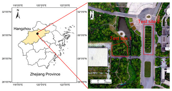
Figure 1.
Location of the study area.
Two test sites were selected to evaluate the performance of the proposed approach. The species on test site 1 consist of Cinnamomum chekiangense, sweetgum, Michelia maudiae, pine, etc. The predominant species on test site 2 are ginkgo and Cinnamomum chekiangense, mixed with sweet olive, pine, etc. Test site 1 is characterized by a large variation in crown size and irregular tree distribution. Test site 2 has a smaller variation in crown size, within which the trees are regularly distributed. The field survey was conducted in November 2020. For each tree within the test sites, the position (x, y coordinates) was measured using an RTK-GNSS and the species was simultaneously recorded. The trees on the test sites can be grouped into dominant, codominant, intermediate, and suppressed ones [37]. The dominant trees are the tallest trees in the neighborhood or isolated trees. The codominant trees are similar trees in a group. The intermediate trees are the ones close to larger trees and their crowns are partially covered. The suppressed trees are located under larger trees and are totally covered. Within test sites 1 and 2, a total of 48 and 39 trees were recorded respectively, including dominant, codominant, and intermediate trees. The suppressed trees were not included due to their invisibility from the CHM. Each tree crown was delineated manually from a supplementary orthophoto acquired in 2019. A circle centered at the tree position was used to represent the crown and the circle diameter was extracted to indicate the crown size. The minimum crown diameters on test sites 1 and 2 are approximately 1.5 and 3 m, respectively.
The aerial survey was conducted in July 2020. The LiDAR data were collected using a DJI Matrice 600 Pro, which carried a Velodyne VLP-16 laser scanner. The LiDAR sensor has a measurement range of 100 m and can generate up to 300,000 points/second at dual return mode across a 360° horizontal field of view and a 30° vertical field of view. During the LiDAR data acquisition, the flight height was approximately 100 m above ground, resulting in a point cloud with average density of approximately 160 points per m2. Direct georeferencing was applied using a GNSS receiver.
2.2. Data Preprocessing
A preprocessing workflow was performed for the raw LiDAR data. Firstly, the iterative filtering and thresholding method proposed in [38] was used to extract ground points. The ground points were then interpolated to create a 0.5 m resolution digital terrain model (DTM) using the Kriging algorithm. Subsequently, the LiDAR point cloud was normalized by subtracting the DTM from the Z coordinates of the raw LiDAR data. The normalized point cloud was then utilized to generate a CHM with 0.25 m resolution by assigning each cell the above-ground height of the highest return within this cell. The cells of missing data were interpolated using the surrounding cells. Finally, a Gaussian smoother and an average smoother were applied on the CHM respectively to smooth out data noise contained in the CHM. The smoother parameters include sliding window size and standard deviation of Gaussian smoother and sliding window size of average smoother. The values of smoother parameters were selected following other related studies [3,30] and are listed in Table 1.

Table 1.
List of parameters and their values used in the proposed approach on test sites 1 and 2.
2.3. Tree Detection Approach
In this paper, an individual tree detection approach based on crown morphology information is proposed. The strategy is to extract as many LMs as possible using a fixed-size LM filter window size and then filter the initially extracted LMs based on crown morphology information. Firstly, a LM filter with a fixed-size sliding window is applied on the CHM to extract LMs. The number of extracted LMs is closely related to the LM filter window size. A small LM filter size allows small trees to be detected, but possibly retains the LMs caused by surface irregularities. A large-size LM filter is unable to detect small trees but can filter out more LMs caused by surface irregularities. In this study, we define the LM filter size according to the minimum crown size. The LM filter size should be smaller than or close to the minimum crown size. Subsequently, crown morphology is described by profile curvature, a morphometric variable commonly applied in terrain analysis. Due to the sensitivity of profile curvature to data noise [39], a spatial autocorrelation statistic, local Gi*, is utilized to quantify the spatial pattern of convex morphology of tree crowns and extract cell clusters representing significant convex morphology. Finally, the initially extracted LMs are filtered depending on the crown morphology information. A score is calculated based on local Gi* values and assigned to each initially extracted LM. The LMs with scores lower than a threshold are filtered out. Then, for each cell cluster containing more than one LM, a new LM filter window size is calculated and applied on each LM within the cell cluster to remove those that are no more the highest within the new windows. The LMs that are retained in the final result represent treetops. The whole workflow of the proposed approach is shown in Figure 2.
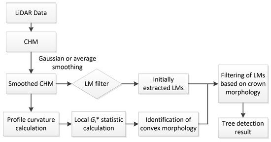
Figure 2.
Workflow of the proposed tree detection approach.
2.3.1. Description and Identification of Crown Morphology
On the basis of in situ observation, tree crowns are generally characterized by an outward curving shape [10]. To describe this shape feature, a morphometric variable, profile curvature, is adopted. Profile curvature measures the rate of change of slope gradient in the direction of maximum change, i.e., slope direction [40]. For a surface z = f(x, y), profile curvature is defined as [41]:
where fx and fy are first-order partial derivatives; fxx, fyy, and fxy are second-order partial derivatives. A positive profile curvature indicates the surface is convex in the slope direction, while a negative value indicates a concave morphology. The profile curvature is calculated on a cell-by-cell basis. For each CHM cell, a fourth-order polynomial is fit to a piecewise continuous surface within a 3 × 3 window centered on this cell and its derivatives are used to calculate the profile curvature [40].
Although profile curvature is capable of describing the outward curving shape of tree crowns, it is sensitive to data noise. The ‘pepper and salt’ appearance will be present if all cells with positive curvature values are extracted (Figure 3). Within a tree crown characterized by an outward curving shape, large positive curvature values tend to cluster. Therefore, the convex morphology of tree crowns can be identified through recognizing the local spatial pattern of clustering of large positive curvature values. In this study, local Gi* statistic is adopted to recognize such a spatial pattern. Let {z1, z2, …, zn} be a set of observations of a random variable acquired on different locations (xi, yi) (i = 1, 2, …, n) over space. Local Gi*, an indicator of local spatial association among observation values around the spatial location i, is defined by [42]:
where W is a n-by-n weight matrix, and s are the mean and the standard deviation of all observations, respectively. In this case, the observations are profile curvature values calculated on the CHM. The spatial weight matrix W defines spatial relationship among observations. A typical method to construct the matrix W for identifying spatial patterns is assigning a weight of one to the observations within a neighborhood of location i, while a weight of zero to others [43,44]. In this study, the spatial weight matrix is constructed based on a distance threshold D, which can be defined as:
where dij represents the distance between the target location i and the neighboring location j. A large distance threshold D results in a large-size neighborhood, enabling a large-scale spatial pattern to be recognized. Multi-scale spatial patterns can be revealed by local Gi* through varying the distance threshold [45,46,47]. For a forest containing trees of multiple species and varying crown sizes, using a single distance threshold is inadequate to recognize the morphology of both small-size trees with regular shape and large-size trees with irregular canopy surface. Therefore, on each cell, a series of distance threshold values are employed and multiple local Gi* values are calculated, amongst which the maximum local Gi* value is recorded. The series of distance threshold values are selected based on the minimum crown size. Theoretically, the maximum distance threshold should not exceed the minimum crown size. For a small intermediate tree, when a distance threshold larger than its crown size is used, its spatial pattern will be concealed by the patterns of neighboring large trees.
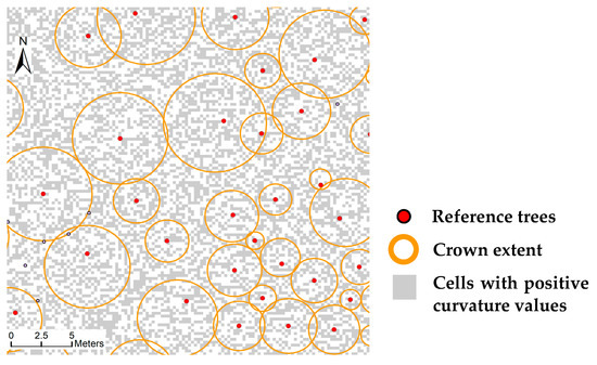
Figure 3.
Extraction of cells with positive profile curvature values.
A large positive local Gi* indicates a local spatial pattern of clustering of large positive profile curvature values, while a large negative one indicates clustering of large negative curvature values. The significance of a local spatial pattern can be measured by means of a statistical significance test. If the neighborhood size is larger than 8 observations, the resultant distribution of local Gi* is normal [48]. The statistic defined by Equation (2) is in a Z-score standardized form. Consequently, to recognize significant spatial patterns, the local Gi* values are directly compared with the critical value under a specified significance level. If a local Gi* value is beyond the critical value, the local spatial pattern is statistically significant [49]. In this study, to recognize the convex morphology of tree crowns, all cells with positive local Gi* values beyond the critical value under a specified significance level are extracted. Figure 4a shows an example of cell extraction. The local Gi* values calculated on the cell containing the LM inside the red rectangle are shown in Figure 4b. With a maximum distance threshold of 1.5 m and an interval equal to the CHM cell size, five distance thresholds (0.5, 0.75, 1.0, 1.25, and 1.5 m) are adopted to calculate local Gi*. The minimum distance threshold is 0.5 m and the distance threshold of 0.25 m is not included so that there is enough number (≥8) of cells used for calculation of local Gi*. On the same cell, the local Gi* values corresponding to the five distance thresholds are all positive. The maximum local Gi* value is 2.72, corresponding to the minimum distance threshold, indicating a small-scale significant pattern of clustering of large positive curvature values. The other local Gi* value beyond the critical value (1.96) corresponds to the maximum distance threshold. That means that around the cell, a large-scale significant pattern is also present. In such a case, the probability that the LM falling in this cell represents an individual tree is high.
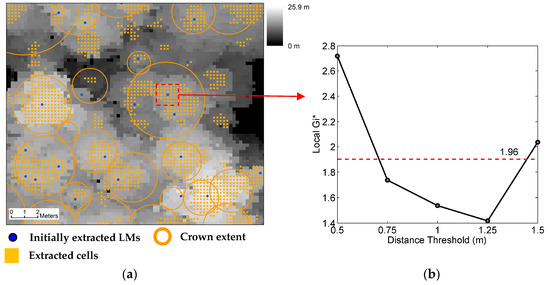
Figure 4.
(a) Extraction of cells with positive local Gi* values beyond the critical value under a significance level of 0.05; (b) Local Gi* values calculated on the cell containing the local maximum (LM) inside the red rectangle. The canopy height model (CHM) resolution is 0.25 m, the LM filter size is 5 × 5, and the maximum distance threshold is 1.5 m.
2.3.2. Filtering of Initially Extracted LMs
The cells extracted through statistical significance tests tend to form clusters (Figure 4). Each initially extracted LM is treated in different ways depending on the following situations:
- (1)
- The LMs outside the extracted clusters are directly removed;
- (2)
- If a cluster contains only one LM, the LM is retained;
- (3)
- If a cluster contains more than one LM, each LM within the cluster is assigned a score that is calculated using the local Gi* values of the cell containing the LM and surrounding 8 cells.
In the third situation, the principle of score definition is that if a LM falls within a local area composed of cells with positive local Gi* values, the local area is characterized by a convex morphology (Figure 5) and the possibility that the LM represents a treetop is high. On each cell within a cluster, multiple local Gi* values corresponding to a series of distance thresholds have been calculated. The number of positive local Gi* (NoP) is counted and recorded for each cell. The score of the ith LM (i = 1, 2, …, m) is given by:
where r and c represent the row and column of the cell containing the target LM, respectively; NNoP≠0 is the total number of the surrounding cells with non-zero NoP values. As explained in Section 2.3.1, the maximum distance threshold determines the number of local Gi* values calculated on each cell. Therefore, the score value is closely related to the maximum distance threshold. As an example, on the cell containing the LM inside the red rectangle in Figure 4, all five local Gi* values are positive and hence its NoP is 5. Around this cell, the NoPs of the 8 neighboring cells are all 5. The target LM’s score that is calculated following Equation (4) is 10. Thus, when a maximum distance threshold of 1.5 m is used, the maximum score value (i.e., full score) is 10. The score value indicates the probability that a LM represents a treetop. A higher score indicates a higher probability. To filter out LMs caused by surface irregularities, a score threshold is applied. All LMs with score values below the threshold are removed.
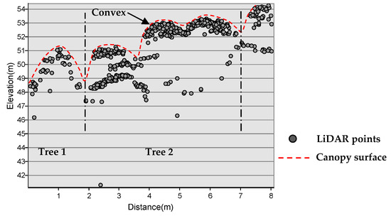
Figure 5.
Point profile indicating the crown morphology of two trees delimited by dash dot lines.
To further filter the LMs, the LM filter window size adaptively varies based on the cell clusters extracted through statistical significance tests. As indicated in Figure 6, the local Gi* values on the cells in dark blue color are lower than 2.576, i.e., the critical value under a significance level of 0.01. These cells are mostly present on the crown boundaries. Therefore, within each cluster containing more than one LM, all the cells with local Gi* values smaller than 2.576 are removed from the cluster. After that, one large-size cluster (e.g., cluster A in Figure 6a) may be divided into several small clusters. If a small cluster contains a single LM, the LM is retained in the final result, while if a small cluster (e.g., cluster in Figure 6c) contains more than one LM, new LM filter window sizes are calculated for each LM according to the extent of the cluster. LM filters with newly calculated window sizes are then centered on the LMs within this cluster. If a LM is still the highest within the new LM filter window, the LM is retained in the result, or else it is removed. During this process, the key step is the calculation of new LM filter window size. As indicated in Figure 6c, starting from the LM in the center, the cluster boundary is searched along four directions and each searching path (black solid line in Figure 6c) has two intersection points with the boundary. For each direction, the distance between the two intersection points is recorded and four distances are finally recorded for this LM. The four distances are rearranged in ascending order. If the minimum distance is larger than the initial LM filter window size (7 cells × 7 cells in Figure 6), the minimum distance is taken as the new LM filter window size.
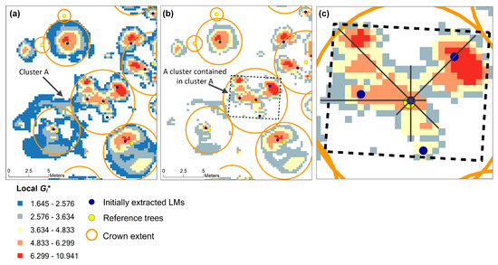
Figure 6.
(a) Extraction of cells under a significance level of 0.10; (b) Removal of all cells with local Gi* values smaller than 2.576 (critical value under significance level of 0.01); (c) Enlargement of the cluster highlighted by a black rectangle in (b) and calculation of new LM filter window size along four directions. The CHM resolution is 0.25 m, the LM filter size is 7 × 7, and the maximum distance threshold is 1.5 m.
2.3.3. Parameter Setting
The parameters in the approach can be divided into two groups: parameters related to LM extraction and parameters related to filtering of LMs based on crown morphology. The first group includes smoother parameters and LM filter window size, while the second group includes maximum distance threshold (maxD), significance level, and score threshold. The parameter values for both test sites are listed in Table 1. The LM filter size and maxD are smaller than or close to the minimum crown size.
2.3.4. Accuracy Assessment
Following the accuracy assessment method in other studies [15], recall (r), precision (p), and F-score (F) as the overall accuracy are calculated using the following equations, respectively:
where TP is the number of correctly detected trees, i.e., true positives; FN is the number of undetected reference trees, i.e., false negatives; FP is the number of incorrectly detected trees, i.e., false positives. Since both tree positions and crown extents have been recorded, the LM closest to the reference tree position within each crown is regarded as a true positive, while the rest of LMs are regarded as false positives. Recall is a measure of tree detection rate and omission error. A larger recall means higher detection rate and lower omission error. Precision is a measure of commission error. A higher precision means smaller commission error.
2.4. Comparison with Existing Method
Our approach is compared with the tree detection algorithm in Fusion software [50]. This algorithm is similar to that reported in [26]. It applies a variable-size window to identify LMs as representative of treetops. The window size is adaptively adjusted based on the crown size estimated using the following equation:
where width is the estimated crown width, ht is the height of the surface at the center of the sliding window. The equation coefficients should be estimated using regression analysis based on the field survey data on tree height and crown diameter [26]. We manually extracted the tree height and crown diameter data on the two test sites. Within a specified area around each reference tree position, the above-ground height of the highest LiDAR point is recorded as the tree height. In Section 2.1, circles were delineated from an orthophoto to represent crown extent. The circle diameter was used as crown diameter. The quadratic regression analysis results for both test sites are given in Figure 7. No significant regression relationship between tree height and crown width can be found both on test sites 1 and 2. Therefore, the default equation coefficients in the Fusion software were adopted to apply the variable-size LM filter. In addition, an average smoother can be applied on the CHM in the software. The smoother sizes adopted in this study can be found in Table 1.
width = A + B × ht + C × ht2 + D × ht3 + E × ht4 + F × ht5,
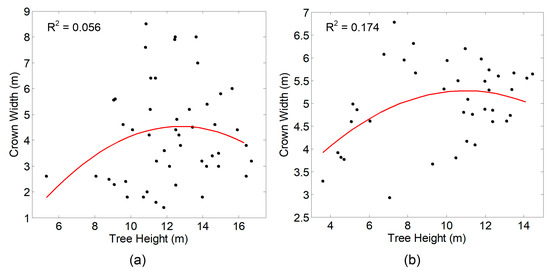
Figure 7.
Quadratic regression model between tree height and crown diameter data derived from test site 1 (a) and test site 2 (b).
3. Results
3.1. Sensitivity Analysis
In this study, the sensitivity of the tree detection approach to parameter values was analyzed. Different combinations of parameter values were applied to derive individual tree detection results and recall, precision, F-score were calculated for the results. Firstly, the values of LM extraction-related parameters varied and other parameter values were fixed. The parameter values for comparison on test site 1 are listed in Table 2. The recall and F-score values generated by using each combination of parameter values are shown in Table 2 and Figure 8.
Table 2.
List of LM extraction-related parameter values and corresponding tree detection results for comparison on test site 1. The values of the parameters related to filtering of initially extracted LMs were fixed. MaxD = 1.5 m, significance level = 0.10, and score threshold = 9.
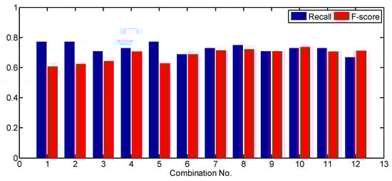
Figure 8.
The effects caused by changing LM extraction-related parameter values on test site 1. The parameter values for each combination can be found in Table 2. MaxD = 1.5 m, significance level = 0.10, and score threshold = 9.
As shown in Table 2 and Figure 8, as the smoothing degree of CHM increased, the detection rate (recall) decreased and the F-score increased. For Gaussian smoother, the smoother size increased from 3 × 3 to 5 × 5 and σ increased from 0.25 to 0.5 m. When a 5 × 5 LM filter was adopted (combinations 1 to 4), the detection rate decreased from 77.1% to 72.9%, while the F-score increased from 60.2% to 70.7%. When a 7 × 7 LM filter was adopted (the 7th to 10th combinations), the detection rate did not increase, while the F-score increased from 71.4% to 73.7%. For average smoother, when a 5 × 5 LM filter was adopted and the smoother size increased from 3 × 3 (the 5th combination) to 5 × 5 (the 6th combination), the detection rate decreased from 77.1% to 68.8%, while the F-score increased from 62.7% to 68.8%. When a 7 × 7 LM filter was adopted and the smoother size increased from 3 × 3 (the 11th combination) to 5 × 5 (the 12th combination), the detection rate decreased from 72.9% to 66.7%, while the F-score increased from 70.7% to 71.1%. A higher smoothing degree induced more details of CHM to be smoothed out, including both true treetops and surface irregularities.
The LM filter size also had an effect on the tree detection results. The detection rates generated by using a 5 × 5 LM filter are higher or equal to the detection rates generated by using a 7 × 7 LM filter. A few LMs related to treetops of small-size crowns could not be extracted when the LM filter size increased. All F-scores generated by using a 7 × 7 LM filter are higher than those generated by using a 5 × 5 LM filter. This is because when a larger-size LM filter was used, fewer LMs due to surface irregularities were extracted. It should be noticed that when the LM filter size increased from 5 × 5 to 7 × 7, the differences in detection rate and F-score among the combinations became smaller. It means that when a larger-size LM filter was used, the effects of smoother parameters on the tree detection results became smaller. Actually, the 7 × 7 LM filter size is slightly larger than the minimum crown size (1.5 m) on test size 1. This proves that a LM filter size approaching the minimum crown size is reasonable. In addition, the comparison between the results of Gaussian smoother and average smoother indicates that the highest F-score generated by a Gaussian smoother is larger than the one generated by an average smoother regardless of LM filter size used.
Then, the effects caused by changing the values of parameters related to filtering of LMs based on crown morphology were analyzed. For the 12 combinations of parameter values in Table 2, the recall and F-score values generated by using a maxD of 1.0 m were subtracted from the ones generated by using a maxD of 1.5 m. The difference values indicate the effects caused by changing the maxD value from 1.0 to 1.5 m. A positive difference means an increase of detection rate or F-score. The calculated difference values are shown in Figure 9. As shown in the figure, when maxD varied from 1.0 to 1.5 m, the detection rates increased or decreased. The difference values of detection rate are mostly +/−2.1% and the largest one (−6.2%) was generated by using a 5 × 5 average smoother and a 5 × 5 LM filter (the 6th combination). In contrast, all difference values of F-score are positive, meaning that more LMs due to surface irregularities were filtered out when a 1.5 m maxD was used. When a larger maxD was adopted, the spatial pattern of crown morphology in larger-size extent was identified and the sizes of the cell clusters extracted from significance tests became larger, leading to the acquisition of a larger-size LM filter window and more LMs being filtered out. The 1.5 m maxD equals the minimum crown size on test site 1, proving that the parameter selection rule that maxD should approach the minimum crown size is appropriate.
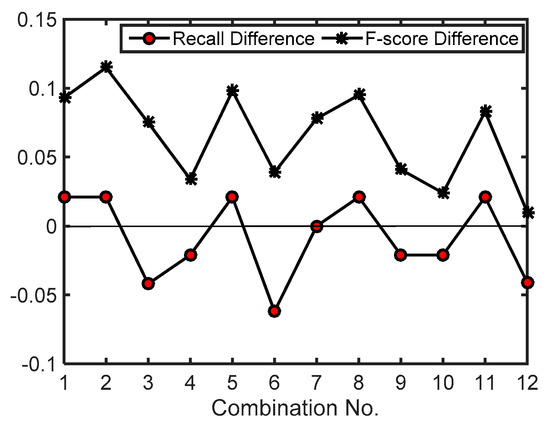
Figure 9.
The effects caused by changing maxD value on test site 1. Recall (F-score) difference is the product of the recall (F-score) generated by using a maxD of 1.5 m minus the one generated by using a maxD of 1.0 m. The parameter values for each combination can be found in Table 2. Significance level = 0.10. For maxD = 1.0 m, score threshold = 5.5. For maxD = 1.5 m, score threshold = 9.
In the same way, for the 12 combinations of parameter values in Table 2, the recall and F-score values generated by using a significance level of 0.10 were subtracted from the ones generated by using a significance level of 0.05. The differences indicate the effects caused by changing the significance level from 0.10 to 0.05. A positive difference means an increase of detection rate or F-score. The calculated difference values are shown in Figure 10. As shown in the figure, the detection rates remained the same or had a minor increase (2.1%). In contrast, almost all F-score values decreased. This is because when the significance level varied from 0.10 to 0.05, fewer cells were extracted through significance tests and one large-size cluster derived under a significance level of 0.10 became several smaller-size clusters under a significance level of 0.05. Within the smaller-size clusters, the single LMs related to treetops or caused by surface irregularities were retained in the final result.
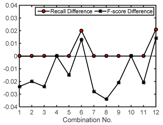
Figure 10.
The effects caused by changing significance level on test site 1. Recall (F-score) difference is the product of the recall (F-score) generated by using a significance level of 0.05 minus the one generated by using a significance level of 0.10. The parameter values for each combination can be found in Table 2. MaxD = 1.5 m, and score threshold = 9.
The effects caused by changing the score threshold were also evaluated. The 1st, 5th, and 10th combinations in Table 2 were applied and two maxD values (1.0 and 1.5 m) were utilized. For maxD of 1.0 m, the full score calculated following Equation (4) is 6 and the score thresholds ranging from 1 to 5.5 were applied. The F-score values of the corresponding tree detection results were calculated and are shown in Figure 11a. As indicated in the figure, the F-score values generated by using the combination 10 were unaffected by the score threshold. As the score threshold increased, the F-score values generated by using combinations 1 and 5 also increased and the maximum F-score values were obtained when a score threshold of 5.5 was used. For maxD of 1.5 m, the full score calculated following Equation (4) is 10 and the score thresholds ranging from 1 to 9.5 were applied. The F-score values of the corresponding tree detection results are shown in Figure 11b. The figure indicates that the F-score values generated by using the combination 10 were unaffected by the score threshold. The F-score values generated by using combination 1 increased with the score threshold and the maximum F-score value was derived when the score threshold equaled 9. The F-score values generated by using combination 5 also increased with the score threshold and the maximum F-score value was derived when a score threshold of 9.5 was used. It can be inferred from Figure 11 that a score threshold approximately equaling to the product of a multiplier of 0.9 and the full score is appropriate for tree detection on test site 1.
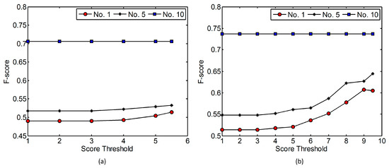
Figure 11.
The effects caused by changing score threshold on test site 1: (a) MaxD = 1.0 m, significance level = 0.10; (b) MaxD = 1.5 m, significance level = 0.10. The 1st, 5th, and 10th combinations in Table 2 were applied.
The parameter values for comparison on test site 2 are listed in Table 3. The recall and F-score values generated by using each combination of parameter values are shown in Table 3 and Figure 12. For Gaussian smoother, as the smoother size and σ increased, the detection rate (recall) decreased. However, when the CHM was smoothed with a higher degree, the F-score did not necessarily increase. No matter which LM filter size was used, the highest F-score was derived by using a 5 × 5 smoother size and a 0.25 m σ, while the lowest F-score was derived by using a 5 × 5 smoother size and a 0.5 m σ. This is different from the comparison result on test site 1. To illustrate the reason, the results generated by using the 9th and 10th combinations of parameter values are shown in Figure 13. The tree highlighted by a white arrow was detected by using the 9th combination of parameter values but undetected when the 10th combination of parameter values was used. The tree crown had an initially extracted LM. During the process of filtering LMs based on crown morphology, all cells with local Gi* values lower than 2.576 (0.01 significance level) were assigned a value of 0. The cell cluster containing this LM was separated from other clusters and the LM was directly retained. However, when the 10th combination of parameter values was used, a large-size cell cluster containing several crowns was generated. A larger LM filter window size that approached the crown size was derived following the method in Section 2.3.2, and the initially extracted LM was removed due to the lower height of this crown. In this case, using a smaller-size LM filter window is more appropriate. For average smoother, when the smoother size increased, the detection rate decreased and the F-score did not necessarily increased for the same reason. By applying a larger-size LM filter, the recall decreased and the F-score increased, regardless of the smoother type. This is the same as the comparison result on test site 1.
Table 3.
List of LM extraction-related parameter values and corresponding tree detection results for comparison on test site 2. The values of the parameters related to filtering of initially extracted LMs were fixed. MaxD = 1.5 m, significance level = 0.10, and score threshold = 9.
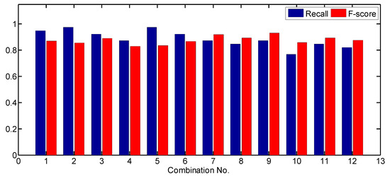
Figure 12.
The effects caused by changing LM extraction-related parameter values on test site 2. The parameter values for each combination can be found in Table 3. MaxD = 1.5 m, significance level = 0.10, and score threshold = 9.
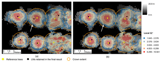
Figure 13.
Tree detection results derived by using the 9th and 10th combinations of parameter values in Table 3: (a) the result generated by using the 9th combination; (b) the result generated by using the 10th combination. The CHM with a 0.25 m resolution is displayed. The cells extracted through significance tests are shown in different colors according to the local Gi* values on each cell.
For the 12 combinations of parameter values in Table 3, the recall and F-score values generated by using a maxD of 1.5 m were subtracted from the ones generated by using a maxD of 2.0 m. The calculated difference values are shown in Figure 14a. The difference values calculated by subtracting the recall and F-score values generated by using a maxD of 1.5 m from the ones generated by using a maxD of 2.5 m are shown in Figure 14b. A positive difference value means the detection rate or F-score increased. As indicated in Figure 14a, when the maxD varied from 1.5 to 2.0 m, the detection rates decreased or remained the same, while the F-score values increased if a 7 × 7 LM filter was adopted. This trend became more obvious when the maxD varied from 1.5 to 2.5 m. The detection rates for all combinations decreased and the F-score values decreased when an 11 × 11 LM filter was adopted, meaning that the use of a large maxD led to both LMs related to treetops and the ones due to surface irregularities being filtered out.
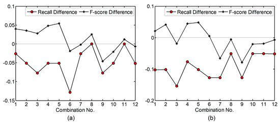
Figure 14.
The effects caused by changing maxD value on test site 2. (a) Recall (F-score) difference as the product of the recall (F-score) generated by using a maxD of 2.0 m minus the one generated by using a maxD of 1.5 m; (b) Recall (F-score) difference as the product of the recall (F-score) generated by using a maxD of 2.5 m minus the one generated by using a maxD of 1.5 m. The parameter values for each combination can be found in Table 3. Significance level = 0.10. For maxD = 1.5 m, score threshold = 9. For maxD = 2.0 m, score threshold = 12. For maxD = 2.5 m, score threshold = 16.
For the 12 combinations of parameter values in Table 3, the recall and F-score values generated by using a significance level of 0.10 were subtracted from the ones generated by using a significance level of 0.05. The calculated difference values are shown in Figure 15. A positive difference means an increase of detection rate or F-score. As indicated in the figure, the detection rates were nearly unaffected but the F-score values mostly increased. This is contrary to the comparison result on test site 1. The largest F-score increase is 3.9%, which was acquired by using a 3 × 3 average smoother and a 7 × 7 LM filter (the 5th combination in Table 3). Through comparing the results of this combination derived by using different significance levels, it can be found that the LMs filtered out by using a significance level of 0.05 were on the boundaries of the cell clusters extracted by using a significance level of 0.10. When the significance level of 0.05 was used, fewer cells were extracted through significance tests and all LMs outside the cell clusters were filtered out. However, under both significance levels, the highest F-score values are the same (93.2%), indicating that if other parameter values are appropriately defined, changing the significance level will only lead to a slight influence (e.g., 0~1% variation in F-score for the 7th to 12th combinations).
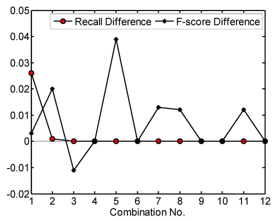
Figure 15.
The effects caused by changing significance level on test site 2. Recall (F-score) difference is the product of the recall (F-score) generated by using a significance level of 0.05 minus the one generated by using a significance level of 0.10. The parameter values for each combination can be found in Table 3. MaxD = 1.5 m, and score threshold = 9.
Finally, the effects caused by changing the score thresholds were analyzed for test site 2. The 1st, 5th, and 10th combinations in Table 3 were applied and two maxD values (1.5 and 2.0 m) were utilized. For maxD of 1.5 m, the full score calculated following Equation (4) is 10 and the score thresholds ranging from 1 to 9.5 were applied. The F-score values of the corresponding tree detection results were calculated and are shown in Figure 16a. The optimal score thresholds for the 1st combination and the 5th combination are 9.5 and 9, respectively. The F-score value generated by using the 10th combination of parameter values was unaffected by the score threshold. For maxD of 2.0 m, the full score calculated following Equation (4) is 14 and the score thresholds ranging from 1 to 13.5 were applied. The F-score values of the corresponding tree detection results are shown in Figure 16b. The optimal score thresholds for the 1st combination and the 5th combination are both 12. The F-score value generated by using the 10th combination of parameter values was unaffected by the score threshold. It can be inferred from the figure that a score threshold approximately equaling to the product of a multiplier of 0.9 and the full score is appropriate for tree detection on test site 2.
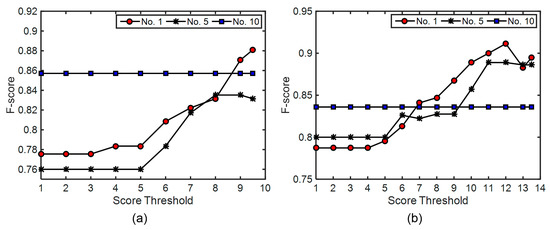
Figure 16.
The effects caused by changing score threshold on test site 2: (a) MaxD = 1.5 m, significance level = 0.10; (b) MaxD = 2.0 m, significance level = 0.10. The 1st, 5th, and 10th combinations in Table 3 were applied.
3.2. Method Performance
For test site 1 with a large variation in crown size and irregular tree distribution, the highest F-score among all results is 73.7%, generated by the combination of 5 × 5 Gaussian smoother, 0.5 m σ, 7 × 7 LM filter, 1.5 m maxD, and significance level of 0.10. When this combination of parameter values was used, the tree detection result was not affected by the variation in score threshold. The tree detection result is shown in Figure 17. The detection rate (recall) is 72.9% and a total of 13 among 48 reference trees were undetected. As indicated in Figure 17a, almost all undetected trees have small-size crowns and are partially covered by neighboring higher trees. Therefore, no LM was initially extracted within their crowns. One exception is crown C in Figure 17b. One LM was initially extracted within its crown but was subsequently filtered out. This is because in the process of recalculation of LM filter size, a larger LM filter window size was derived and the initial LM was no more the highest within the new LM filter window and hence removed. The precision is 74.5%. A total of 10 LMs (e.g., the blue ones in crowns A and B in Figure 17b) caused by surface irregularities were filtered out based on crown morphology and 12 ones were retained in the final result. Within some large-size crowns such as crowns D and E in Figure 17c, more than one LM was retained in the final result. These trees are of ever-green broadleaf species and have many large branches and irregular crown surfaces. Thus, within their crowns, the cell clusters extracted through significance tests had complex shapes, which affected the calculation of new LM filter window size and the subsequent filtering of LMs.
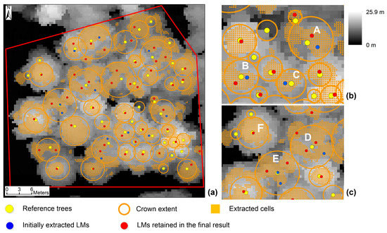
Figure 17.
Tree detection result on test site 1 using the proposed approach. (a) Whole extent of test site 1; (b,c) Enlarged samples. The cells extracted through significance tests are shown in orange color. The CHM resolution is 0.25 m, the Gaussian filter size is 5 × 5, σ is 0.5 m, the LM filter size is 7 × 7, the maxD is 1.5 m, and the significance level is 0.10. The result was unaffected by the variation in score threshold.
For test site 2 with a smaller variation in crown size and regular tree distribution, the highest F-score among all results is 93.2%, generated by the combination of 5 × 5 Gaussian smoother, 0.25 m σ, 11 × 11 LM filter, 1.5 m maxD, and significance level of 0.10. The result was not affected by the variation in score threshold. The tree detection result is shown in Figure 18. The detection rate (recall) is 87.2% and a total of 5 among 39 reference trees were undetected. The sizes of these undetected crowns vary from 3.8 to 6.0 m, not including the minimum crown size (3.0 m) in this test site. As shown in Figure 18a, no LM was initially extracted within the extents of the undetected crowns. One exception is crown B in Figure 18c, whose initially extracted LMs were filtered out. We checked the tree heights of these undetected crowns and their neighbors and found that these undetected crowns were lower than their neighbors. As an example, the tree height of crown B in Figure 18c is 10.0 m and the tree heights of the two closest neighbors are 13.3 and 13.5 m. Their crowns have an overlap. A larger-size LM filter window was derived during the process of filtering LMs based on crown morphology. The treetop of crown B was not the highest within the new window and hence removed. The precision is 100%. A total of 4 LMs (e.g., the blue ones outside crown A in Figure 18b) caused by surface irregularities were filtered out based on crown morphology. The number is small since few LMs caused by surface irregularities were initially extracted. In comparison with the result in Figure 17, both recall and precision are much higher on test site 2. This is due to the homogeneous tree properties on test site 2. Because most trees have similar crown sizes, a LM filter with a window size (11 × 11) approaching the mean crown size (2.5 m) induced high detection rates and low commission errors. However, on test site 1, the difference between the minimum (1.5 m) and maximum (8.5 m) crown sizes is large and the LM filter size (7 × 7) defined based on the minimum crown size induced higher commission errors.
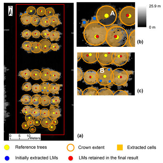
Figure 18.
Tree detection result on test site 2 using the proposed approach. (a) Whole extent of test site 2; (b,c) Enlarged samples. The cells extracted through significance tests are shown in orange color. The CHM resolution is 0.25 m, the Gaussian filter size is 5 × 5, σ is 0.25 m, the LM filter size is 11 × 11, the maxD is 1.5 m, and the significance level is 0.10. The result was unaffected by the variation in score threshold.
3.3. Method Comparison
The variable-size window LM extraction algorithm in Fusion software was applied on both test sites. A 3 × 3 and a 5 × 5 average smoother were applied on the 0.25 m CHM respectively before the LM identification and the best results (highest F-score) are displayed in Table 4 and Figure 19. As a comparison, the tree detection results of the proposed approach derived by using the optimal combinations of parameter values were shown in the table. Since only the average smoother is available in Fusion, the best results of the proposed approach generated by using the average smoother are also shown in the table. It should be noticed that the highest F-score values were derived by using not only one combination of parameter values for both test sites 1 and 2. As indicated in Table 4, the proposed approach generated slightly better results than the variable-size window LM extraction algorithm. On test site 1, although the difference (1.2%) in F-score between the proposed approach and the variable-size window algorithm is slight, a much higher detection rate (72.9%) was derived by using the proposed approach. This is because the proposed approach utilized a small-size LM filter to extract LMs and then performed filtering of the initially extracted LMs based on crown morphology. Therefore, both higher detection rate and higher commission error (lower precision) were derived. The variable-size window algorithm adjusted the LM filter window size according to the surface height. Due to the insignificant relationship between tree heights and crown sizes (Figure 7) and crown overlapping on both test sites, it was difficult to determine the appropriate window sizes for those trees with large crown sizes but lower tree heights and those trees with small crown sizes but larger tree heights.
Table 4.
Individual tree detection results derived by using the proposed approach and the algorithm in Fusion software.
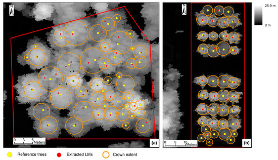
Figure 19.
Tree detection results on test sites 1 and 2 using the algorithm in Fusion software: (a) Test site 1; (b) Test site 2. The CHM resolution is 0.25 m. The parameter values applied in the algorithm can be found in Table 4.
4. Discussion
4.1. Rules for Parameter Setting
For the proposed approach, the effects caused by changing the parameter values on the tree detection results have been thoroughly investigated. The parameters used in the approach were divided into two groups: the parameters related to local maximum (LM) extraction and the parameters related to filtering of the initially extracted LMs based on crown morphology. Even though the proposed approach was found to be more or less sensitive to the parameter values, rules related to parameter setting can be derived. For forests with different structures, there is difference in the rules. Test site 1 is characterized by irregular tree distribution and large variation in crown size, while test site 2 is characterized by regular tree distribution and small variation in crown size. The rules are as follows:
- Because the results (F-score) derived by using a Gaussian smoother were generally better than those derived by using an average smoother on both test sites, the Gaussian smoother is preferred. A larger smoother size and a higher standard deviation for Gaussian smoother should be utilized to smooth out the surface irregularities contained in CHM. However, for those forests with structures similar to test site 2, a high smoothing degree of CHM will lead to the LMs within large-size crowns that have an overlap with neighboring crowns and are lower than neighbors being filtered out. In such a case, the CHM should be smoothed with a slightly lower degree.
- The LM filter window size should approach the minimum crown size so that as many small-size crowns as possible can be detected.
- A maximum distance threshold (maxD) that approaches the minimum crown size is appropriate for the forests with a large variation in crown size. However, for those forests with relatively homogeneous tree properties like test site 2, using a maxD that approaches the minimum crown size leads to both LMs related to treetops and the ones caused by surface irregularities being filtered out and the F-score values could decrease when a large-size LM filter window is adopted. In such a case, a maxD smaller than the minimum crown size should be used.
- The score threshold for filtering initially extracted LMs can be approximately defined as the product of a multiplier of 0.9 and the full score. The full score varies with the maxD value. A larger maxD leads to a larger full score and hence a larger score threshold.
- A significance level of 0.10 is appropriate for both test sites. Although the sensitivity analysis in Section 3.1 indicates that the F-score values slightly increased when the significance level was changed from 0.10 to 0.05 on test site 2, the highest F-score values among all combinations of parameter values were the same under both significance levels. Therefore, if other parameter values are appropriately defined, the effects caused by changing the significance level can be neglected.
4.2. Advantage and Limitation
This study focuses on individual tree detection using unmanned aerial vehicle (UAV) LiDAR data in subtropical mixed broadleaf forests in urban scenes, which are characterized by complex forest structure and large variation in crown size. Tree detection solely based on height is difficult and complementary information is used in this study. A novel approach based on crown morphology information is proposed for individual tree detection using UAV LiDAR data. The strategy is using a LM filter whose window size approaches the minimum crown size to extract as many LMs as possible and then using the crown morphology identified based on local Gi* statistics to filter out LMs caused by surface irregularities in CHM. The LMs retained in the final result represent treetops. The approach does not need to collect field survey data to obtain such prior knowledge as the relationship between crown size and tree height. Actually, this relationship has been proved to be insignificant for both test sites in this study. Therefore, in comparison with other methods that require prior knowledge [26,27,28], the proposed approach is advantageous to tree detection in subtropical mixed broadleaf urban forests that have similar characteristics to the test sites.
Because the studies on subtropical mixed broadleaf urban forests are very few, a popular variable-size window LM extraction algorithm [50] was used to compare with the proposed approach. The comparison result indicates that the proposed approach obtained slightly higher tree detection accuracy (F-score) than the variable-size window LM extraction algorithm. Although the commission error was relatively large, much higher detection rates were derived by using the proposed approach on test site 1 characterized by irregular tree distribution and large variation in crown size. An advantage of a high detection rate is that complementary information apart from crown morphology can be employed to further filter the LMs to improve the tree detection accuracy. The feasibility of using point density [36] or other point cloud metrics as complementary information for filtering LMs should be investigated in further studies. Moreover, an observation can be derived from the results shown in Section 3.1 and Section 3.2 that the cell clusters extracted through significance tests approximate the crown extents and the cells around treetops have the largest local Gi* values. Therefore, in the further study, the method for segmenting the cell clusters based on the spatial pattern of local Gi* values should be investigated.
The limitation of the proposed approach is that it is still relatively sensitive to the parameter setting, including smoother parameters, LM filter window size, and parameters related to filtering of LMs based on crown morphology. Even though some rules for parameter setting have been proposed in this study, it is difficult to find a balance among the parameters and to automatically obtain the optimal combination of parameter values for each test site characterized by different forest structures. The use of complementary information apart from crown morphology to further filter the LMs retained in the result may help reduce the sensitivity of the approach to the parameter setting. In addition, too few test sites were used in this study due to the limitation of data acquisition. In further studies, more test sites with different characteristics should be established to investigate the parameter setting rules.
5. Conclusions
In this paper, a novel tree detection approach is proposed for subtropical mixed broadleaf forests in urban scenes using unmanned aerial vehicle (UAV) LiDAR data. The proposed approach firstly applies a fixed-size window local maximum (LM) filter to extract LMs and then identifies the spatial pattern of convex crown morphology based on local Gi* statistics to filter out LMs caused by surface irregularities in CHM. The LMs retained in the final result represent treetops. The proposed approach was applied on two test sites located in a university campus using UAV LiDAR data to evaluate its performance. The two test sites are characterized by different forest structures. Through a sensitivity analysis, the optimal combination of parameter values for each test site was obtained and the rules for parameter setting were also derived. By using the optimal combinations of parameter values, the highest F-score values for test sites 1 and 2 were 73.7% and 93.2%, respectively, which were slightly better than the results derived by using a variable-size window tree detection algorithm. The detection rates on both test sites were also higher than the variable-size window algorithm. Although the rules for parameter setting have been proposed in this study, it is still difficult to automatically determine the optimal combination of parameter values. Complementary information apart from crown morphology should be considered to further filter the LMs retained in the final result to improve the tree detection accuracy. More test sites with different characteristics should be established to investigate the parameter setting rules.
Author Contributions
S.D. and W.X. collectively conceptualized the research and proposed the methodology. S.D. prepared the original draft. W.X. collected the data, prepared the software, and analyzed the results. D.L. and X.C. contributed to the review and editing of the paper. All authors have read and agreed to the published version of the manuscript.
Funding
This research was supported by the research fund of Zhejiang A&F University (2015FR023).
Data Availability Statement
Data sharing is not applicable to this article.
Acknowledgments
The authors acknowledge Yinyin Zhao, Demin Li and Zihao Fang (Zhejiang A&F University) for their help during the fieldwork.
Conflicts of Interest
The authors declare no conflict of interest.
References
- Gomes, M.; Maillard, P. Detection of Tree Crowns in Very High Spatial Resolution Images. Environ. Appl. Remote Sens. 2016. [Google Scholar] [CrossRef]
- Bettinger, P.; Boston, K.; Siry, J.P.; Grebner, D.L. Forest Management and Planning, 2nd ed.; Academic Press: London, UK, 2017. [Google Scholar]
- Kwong, I.H.Y.; Fung, T. Tree height mapping and crown delineation using LiDAR, large format aerial photographs, and unmanned aerial vehicle photogrammetry in subtropical urban forest. Int. J. Remote Sens. 2020, 41, 5228–5256. [Google Scholar] [CrossRef]
- Popescu, S.C. Estimating biomass of individual pine trees using airborne LiDAR. Biomass Bioenerg. 2007, 31, 646–655. [Google Scholar] [CrossRef]
- Holmgren, J.; Persson, Å.; Söderman, U. Species identification of individual trees by combining high resolution LiDAR data with multispectral images. Int. J. Remote Sens. 2008, 29, 1537–1552. [Google Scholar] [CrossRef]
- Zhang, W.; Ke, Y.; Quackenbush, L.J.; Zhang, L. Using error-in-variable regression to predict tree diameter and crown width from remotely sensed imagery. Can. J. For. Res. 2010, 40, 1095–1108. [Google Scholar] [CrossRef]
- Harikumar, A.; Bovolo, F.; Bruzzone, L. A Local Projection-Based Approach to Individual Tree Detection and 3-D Crown Delineation in Multistoried Coniferous Forests Using High-Density Airborne LiDAR Data. IEEE Trans. Geosci. Remote Sens. 2019, 57, 1168–1182. [Google Scholar] [CrossRef]
- Wagner, F.H.; Ferreira, M.P.; Sanchez, A.; Hirye, M.C.M.; Zortea, M.; Gloor, E.; Phillips, O.L.; de Souza Filho, C.R.; Shimabukuro, Y.E.; Aragão, L.E.O.C. Individual tree crown delineation in a highly diverse tropical forest using very high resolution satellite images. ISPRS J. Photogram. Remote Sens. 2018, 145B, 362–377. [Google Scholar] [CrossRef]
- Qiu, L.; Jing, L.; Hu, B.; Li, H.; Tang, Y. A New Individual Tree Crown Delineation Method for High Resolution Multispectral Imagery. Remote Sens. 2020, 12, 585. [Google Scholar] [CrossRef]
- Zhen, Z.; Quackenbush, L.J.; Zhang, L. Trends in Automatic Individual Tree Crown Detection and Delineation—Evolution of LiDAR Data. Remote Sens. 2016, 8, 333. [Google Scholar] [CrossRef]
- Næsset, E.; Økland, T. Estimating tree height and tree crown properties using airborne scanning laser in a boreal nature reserve. Remote Sens. Environ. 2002, 79, 105–115. [Google Scholar] [CrossRef]
- Dalponte, M.; Coops, N.C.; Bruzzone, L.; Gianelle, D. Analysis on the use of multiple returns lidar data for the estimation of tree stems volume. IEEE J. Sel. Top. Appl. Earth Obs. Remote Sens. 2010, 2, 310–318. [Google Scholar] [CrossRef]
- Huang, H.; Li, X.; Chen, C. Individual Tree Crown Detection and Delineation from Very-High-Resolution UAV Images Based on Bias Field and Marker-Controlled Watershed Segmentation Algorithms. IEEE J. Sel. Top. Appl. Earth Obs. 2018, 11, 2253–2262. [Google Scholar] [CrossRef]
- Wallace, L.; Lucieer, A.; Watson, C.S. Evaluating tree detection and segmentation routines on very high resolution UAV LiDAR data. IEEE Trans. Geosci. Remote Sens. 2014, 52, 7619–7628. [Google Scholar] [CrossRef]
- Jaskierniak, D.; Lucieer, A.; Kuczera, G.; Turner, D.; Lane, P.N.J.; Benyon, R.G.; Haydon, S. Individual tree detection and crown delineation from Unmanned Aircraft System (UAS) LiDAR in structurally complex mixed species eucalypt forests. ISPRS J. Photogramm. Remote Sens. 2021, 171, 171–187. [Google Scholar] [CrossRef]
- Reitbergera, J.; Schnörrb, C.l.; Krzysteka, P.; Stilla, U. 3D segmentation of single trees exploiting full waveform LIDAR data. ISPRS J. Photogram. Remote Sens. 2009, 64, 561–574. [Google Scholar] [CrossRef]
- Paris, C.; Valduga, D.; Bruzzone, L. A Hierarchical Approach to Three-Dimensional Segmentation of LiDAR Data at Single-Tree Level in a Multilayered Forest. IEEE Trans. Geosci. Remote Sens. 2016, 54, 1–14. [Google Scholar] [CrossRef]
- Hyyppä, J.; Kelle, O.; Lehikoinen, M.; Inkinen, M. A segmentation-based method to retrieve stem volume estimates from 3-D tree height models produced by laser scanners. IEEE Trans. Geosci. Remote Sens. 2001, 39, 969–975. [Google Scholar] [CrossRef]
- Yu, X.; Hyyppä, J.; Vastaranta, M.; Holopainen, M.; Viitala, R. Predicting individual tree attributes from airborne laser point clouds based on the random forests technique. ISPRS J. Photogram. Remote Sens. 2011, 66, 28–37. [Google Scholar] [CrossRef]
- Dalponte, M.; Coomes, D.A. Tree-centric mapping of forest carbon density from airborne laser scanning and hyperspectral data. Methods Ecol. Evol. 2016, 7, 1236–1245. [Google Scholar] [CrossRef]
- Hamraz, H.; Contreras, M.A.; Zhang, J. Vertical stratification of forest canopy for segmentation of understory trees within small-footprint airborne LiDAR point clouds. ISPRS J. Photogramm. Remote Sens. 2017, 130, 385–392. [Google Scholar] [CrossRef]
- Huo, L.; Lindberg, E. Individual tree detection using template matching of multiple rasters derived from multispectral airborne laser scanning data. Int. J. Remote Sens. 2020, 41, 9525–9544. [Google Scholar] [CrossRef]
- Koch, B.; Heyder, U.; Weinacker, H. Detection of Individual Tree Crowns in Airborne Lidar Data. Photogramm. Eng. Remote Sens. 2006, 72, 357–363. [Google Scholar] [CrossRef]
- Aubry-Kientz, M.; Dutrieux, R.; Ferraz, A.; Saatchi, S.; Hamraz, H.; Williams, J.; Coomes, D.; Piboule, A.; Vincent, G. A comparative assessment of the performance of individual tree crowns delineation algorithms from ALS data in tropical forests. Remote Sens. 2019, 11, 1086. [Google Scholar] [CrossRef]
- Ben-Arie, J.R.; Hay, G.J.; Powers, R.P.; Castilla, G.; St-Onge, B. Development of a pit filling algorithm for lidar canopy height models. Comput. Geosci. 2009, 35, 1940–1949. [Google Scholar] [CrossRef]
- Popescu, S.; Wynne, R. Seeing the trees in the forest: Using LIDAR and multispectral data fusion with local filtering and variable window size for estimating tree height. Photogramm. Eng. Remote Sens. 2004, 70, 589–604. [Google Scholar] [CrossRef]
- Coomes, D.A.; Dalponte, M.; Jucker, T.; Asner, G.P.; Banin, L.F.; Burslem, D.; Lewis, S.L.; Nilus, R.; Phillips, O.L.; Phua, M.H.; et al. Area-based vs tree-centric approaches to mapping forest carbon in Southeast Asian forests from airborne laser scanning data. Remote Sens. Environ. 2017, 194, 77–88. [Google Scholar] [CrossRef]
- Sačkov, I.; Hlásny, T.; Bucha, T.; Juriš, M. Integration of tree allometry rules to treetops detection and tree crowns delineation using airborne lidar data. iForest-Biogeosci. For. 2017, 10, 459. [Google Scholar] [CrossRef]
- Strîmbu, V.F.; Strîmbu, B.M. A graph-based segmentation algorithm for tree crown extraction using airborne LiDAR data. ISPRS J. Photogramm. Remote Sens. 2015, 104, 30–43. [Google Scholar] [CrossRef]
- Yang, J.; Kang, Z.; Cheng, S.; Yang, Z.; Akwensi, P.H. An Individual Tree SegmentationMethod Based on Watershed Algorithm and Three-Dimensional Spatial Distribution Analysis from Airborne LiDAR Point Clouds. IEEE J. Sel. Top. Appl. Earth Obs. Remote Sens. 2020, 13, 1055–1067. [Google Scholar] [CrossRef]
- Brandtberg, T.; Warner, T.A.; Landenberger, R.E.; McGraw, J.B. Detection and analysis of individual leaf-off tree crowns in small footprint, high sampling density lidar data from the eastern deciduous forest in North America. Remote Sens. Environ. 2003, 85, 290–303. [Google Scholar] [CrossRef]
- Van Leeuwen, M.; Coops, N.C.; Wulder, M.A. Canopy surface reconstruction from a LiDAR point cloud using Hough transform. Remote Sens. Lett. 2010, 1, 125–132. [Google Scholar] [CrossRef]
- Holmgren, J.; Lindberg, E. Tree crown segmentation based on a geometric tree crown model for prediction of forest variables. Can. J. Remote Sens. 2013, 39, S86–S98. [Google Scholar] [CrossRef]
- Mongus, D.; Žalik, B. An efficient approach to 3d single tree-crown delineation in lidar data. ISPRS J. Photogramm. Remote Sens. 2015, 108, 219–233. [Google Scholar] [CrossRef]
- Naveed, F.; Hu, B.; Wang, J.; Hall, G.B. Individual Tree Crown Delineation Using Multispectral LiDAR Data. Sensors 2019, 19, 5421. [Google Scholar] [CrossRef]
- Latella, M.; Sola, F.; Camporeale, C. A Density-Based Algorithm for the Detection of Individual Trees from LiDAR Data. Remote Sens. 2021, 13, 322. [Google Scholar] [CrossRef]
- Wang, Y.; Hyyppä, J.; Liang, X.; Kaartinen, H.; Yu, X.; Lindberg, E.; Holmgren, J.; Qin, Y.; Mallet, C.; Ferraz, A.; et al. International Benchmarking of the Individual Tree Detection Methods for Modeling 3-D Canopy Structure for Silviculture and Forest Ecology Using Airborne Laser Scanning. IEEE Trans. Geosci. Remote Sens. 2016, 54, 5011–5027. [Google Scholar] [CrossRef]
- Axelsson, P. Processing of laser scanner data—Algorithms and applications. ISPRS J. Photogramm. Remote Sens. 1999, 54, 138–147. [Google Scholar] [CrossRef]
- Shary, P.A.; Sharaya, L.S.; Mitusov, A.V. Fundamental quantitative methods of land surface analysis. Geoderma 2002, 107, 1–32. [Google Scholar] [CrossRef]
- Schmidt, J.; Evans, I.S.; Brinkmann, J. Comparison of polynomial models for land surface curvature calculation. Int. J. Geogr. Inf. Sci. 2003, 17, 797–814. [Google Scholar] [CrossRef]
- Evans, I.S. General geomorphometry, derivatives of altitude, and descriptive statistics. In Spatial Analysis in Geomorphology; Chorley, R.J., Ed.; Methuen & Co.: London, UK, 1972; Chapter 2; pp. 17–90. [Google Scholar]
- Ord, J.K.; Getis, A. Local Spatial Autocorrelation Statistics. Geogr. Anal. 1995, 27, 286–306. [Google Scholar] [CrossRef]
- Boots, B. Local measures of spatial association. Ecoscience 2002, 9, 168–176. [Google Scholar] [CrossRef]
- Lanorte, A.; Danese, M.; Lasaponara, R.; Murgante, B. Multiscale mapping of burn area and severity using multisensor satellite data and spatial autocorrelation analysis. Int. J. Appl. Earth Obs. 2013, 20, 42–51. [Google Scholar] [CrossRef]
- Derksen, C.; Wulder, M.; LeDrew, E.; Goodison, B. Associations between spatially autocorrelated patterns of SSM/I-derived prairie snow cover and atmospheric circulation. Hydrol. Process. 1998, 12, 2307–2316. [Google Scholar] [CrossRef]
- Nelson, A.; Oberthür, T.; Cook, S. Multi-scale correlations between topography and vegetation in a hillside catchment of Honduras. Int. J. Geogr. Inf. Sci. 2007, 21, 145–174. [Google Scholar] [CrossRef]
- Shi, W.; Deng, S.; Xu, W. Extraction of multi-scale landslide morphological features based on local Gi* using airborne LiDAR-derived DEM. Geomorphology 2018, 303, 229–242. [Google Scholar] [CrossRef]
- Griffith, P.; Getis, A.; Griffin, E. Regional patterns of affirmative action compliance costs. Ann. Regional Sci. 1996, 30, 321–340. [Google Scholar] [CrossRef]
- Anselin, L. Local Indicators of Spatial Association-LISA. Geogr. Anal. 1995, 27, 93–115. [Google Scholar] [CrossRef]
- McGaughey, R.J. FUSION/LDV: Software for LIDAR Data Analysis and Visualization. 2018. Available online: http://forsys.sefs.uw.edu/Software/FUSION/FUSION_manual.pdf (accessed on 17 March 2021).
Publisher’s Note: MDPI stays neutral with regard to jurisdictional claims in published maps and institutional affiliations. |
© 2021 by the authors. Licensee MDPI, Basel, Switzerland. This article is an open access article distributed under the terms and conditions of the Creative Commons Attribution (CC BY) license (http://creativecommons.org/licenses/by/4.0/).