Article

Robust Classification Technique for Hyperspectral Images Based on 3D-Discrete Wavelet Transform

1
Research Scholar, Department of Electronics and Communication Engineering, Amrita School of Engineering, Amrita Vishwa Vidyapeetham, Coimbatore 641112, India
2
Department of Electronics and Communication Engineering, Amrita School of Engineering, Amrita Vishwa Vidyapeetham, Coimbatore 641112, India
*
Author to whom correspondence should be addressed.
Remote Sens. 2021, 13(7), 1255; https://doi.org/10.3390/rs13071255
Submission received: 1 February 2021 / Revised: 13 March 2021 / Accepted: 16 March 2021 / Published: 25 March 2021
(This article belongs to the Special Issue Wavelet Transform for Remote Sensing Image Analysis)

Abstract

:
Hyperspectral image classification is an emerging and interesting research area that has attracted several researchers to contribute to this field. Hyperspectral images have multiple narrow bands for a single image that enable the development of algorithms to extract diverse features. Three-dimensional discrete wavelet transform (3D-DWT) has the advantage of extracting the spatial and spectral information simultaneously. Decomposing an image into a set of spatial–spectral components is an important characteristic of 3D-DWT. It has motivated us to perform the proposed research work. The novelty of this work is to bring out the features of 3D-DWT applicable to hyperspectral images classification using Haar, Fejér-Korovkin and Coiflet filters. Three-dimensional-DWT is implemented with the help of three stages of 1D-DWT. The first two stages of 3D-DWT are extracting spatial resolution, and the third stage is extracting the spectral content. In this work, the 3D-DWT features are extracted and fed to the following classifiers (i) random forest (ii) K-nearest neighbor (KNN) and (iii) support vector machine (SVM). Exploiting both spectral and spatial features help the classifiers to provide a better classification accuracy. A comparison of results was performed with the same classifiers without DWT features. The experiments were performed using Salinas Scene and Indian Pines hyperspectral datasets. From the experiments, it has been observed that the SVM with 3D-DWT features performs better in terms of the performance metrics such as overall accuracy, average accuracy and kappa coefficient. It has shown significant improvement compared to the state of art techniques. The overall accuracy of 3D-DWT+SVM is 88.3%, which is 14.5% larger than that of traditional SVM (77.1%) for the Indian Pines dataset. The classification map of 3D-DWT + SVM is more closely related to the ground truth map.

Graphical Abstract

1. Introduction

The importance of HSI has accurate discrimination of different materials in spectral resolution and analysis of a small spatial structure in spatial resolutions [1,2]. The anomaly detection based on the auto encoder (AE) has attracted significant interest in the study of hyperspectral images (HSI). Both spatial and spectral resolution are powerful tools for accurate analysis of the Earth surface. HSI data provide useful information related to size, structure, and elevation. HSI deals with big data because it has huge information available in several bands, and it has a good impact on classifying different urban areas. For the selection of classifiers for processing of fusion, data must satisfy the properties such as (i) accurate and automatic (ii) simple and fast [3,4]. Let 𝑥 be an input attributes, and f(x) be a projecting or mapping function, then, predicted class “y” is given as
y = i = 1 N f ( x i )
According to the Equation (1), x   =   x 1 ,   x 2 ,   x 3 ,     x N , which are the set of attributes 𝑥 to N of sample data [1]. Hyperspectral imaging is highly advanced remote sensing imagery consisting of hundreds of continuous narrow spectral bands compared to traditional panchromatic and multispectral images. Additionally, it allows a better accuracy for object classifications. Discrete wavelet transform (DWT) provides better precision in case of HSI image classification [3]. It is a time-scale methodology that can be used in several applications [3]. Ghazali et al. [4] has developed 2D-DWT feature extraction method and image classifier for hyperspectral data. Chang et al. [5] proposed the improved image denoising method using 2D-DWT for hyperspectral images.
Sparse representation of signals (images, movies or other multidimensional signals) is very important for a wide variety of applications, such as compression, denoising, attribute extraction, estimation, super-resolution, compressive sensing [1], blind separation of mixtures of dependent signals [2] and many others. In most cases, discrete cosine transform (DCT) is applied for sparse representation, and DWT is applicable for both linear transformations and filter bank. Thus, several versions of these transformations are involved in contemporary approaches for signal encoding (MP3...), image compression (JPEG, JPEG2000...), as well as in several other implementations. Low computational complexity is an important benefit of the DWT when it is implemented using wavelet filter banks. Usually, for decomposition and reconstruction, finite support filters are used. For a large class of signals, the wavelet transform offers sparse representation. DWT filter banks, however, have several drawbacks: ringing near discontinuities, shift variance and the lack of decomposition function directionality. A lot of studies and publications have recently focused on solving these issues. Adaptive wavelet filter bank [3,4] is one of the methods for obtaining spectral representation and lower dissipation in the wavelet domain. A lower ringing effect is achieved when the norm of L2 or L1 is minimized by adapting wavelet functions in some neighborhoods of each data sample [5,6]. With the help of dual-tree complex wavelet transform [7], the directionality and shift variance problem may be reduced in high dimensional data. In addition, the adaptive directional lifting-based wavelet adjusts directions on every pixel depending on the image orientation in the neighborhood [8]. Enhancement can be achieved in all implementations using multiple representations. The better quality of the estimation will be provided by more statistical estimators with known properties for the same estimated value. The referred advantages of the wavelet transform motivated us to apply it for HSI classification.
In this work, 3D-DWT features are extracted from HSI data, which has both spatial and spectral information. It has various applications and the ability to collect remote sensed data from visible to near infrared (NIR) wavelength ranges, delivering multi-spectral channels from the same location. An attempt is made to perform hyperspectral data classification using the 3D-DWT. The 3D-DWT features are extracted and applied to the following classifiers: (i) random forest (ii) K-nearest neighbor (KNN) and (iii) support vector machine (SVM). A comparison of results was performed with the same classifiers without DWT features. The aim of this work to exploit both spatial and spectral features using suitable classifiers to provide better classification accuracy. By using 3D-DWT, it is possible to achieve better relative accuracy of about 14.5% compared with classifier without using DWT, which is the contributions of the proposed work.
The rest of the work is organized as follows. Section 2 describes related work. Methodology is elaborated in Section 3. Section 4 deals with results and discussion on various HSI image classification. Conclusions are given in Section 5.

2. Related Work

HSI has a very fine resolution of the spectral information with the use of hundreds of bands. These bands give more information about the spectral details of a scene. Many researchers have attempted to perform HSI image classification using various techniques. First, a classification task that attempts to assign a hyperspectral image pixel into many categories can be converted to several hyperspectral applications. State-of-the-art classification techniques were tried for this role, and appreciable success was achieved for some applications [1,2,3,4]. However, these approaches also tend to face some difficulties in realistic situations. Second, the available labelled training samples in the HSI classification are usually small because of the high cost of image marking [5], which contributes to solve the issue of high-dimension and low sample size classification. Third, considering the high spectral resolution of HSI, the same material may have very different spectral signatures, while different materials may share identical spectral signatures [6].
Various grouping methods have been studied to solve these problems. A primary strategy is to find the critical discriminatory features that gain classification, while reducing the noise embedded in HSIs that impairs classification efficiency. It was pointed out in [7] that spatial information is more relevant in terms of leveraging discriminatory characteristics than the spectral signatures in the HSI classification. Therefore, a pixel-wise classification approach becomes a simple but successful way of applying this technique [4,8] after a spatial-filtering preprocessing stage. Square patch is a representative tool for the strategy of spatial filtering [9,10,11], which first groups the adjacent pixels by square windows and then extracts local window-based features using other subspace learning strategies, such as low-rank matrix factorization [12,13,14,15,16,17], learning dictionary [4,18] and clustering subspace [19]. Compared to the initial spectral signatures, the filtered characteristics derived by the square patch process have less intra-class heterogeneity and greater spatial smoothness, with much decreased noise.
The spectral–spatial method, which incorporates spectral and spatial information into a classifier, except for the spatial filtering method, is another common technique to manipulate spatial information. Unlike the pixel-wise classification approach that does not consider spatial structure details, this approach integrates the local accuracy of the neighboring pixel labels. Such an approach has been suggested to unify the pixel-wise grouping with a segmentation map [20]. In addition, 3D-DWT is also a common technique for a spectral–spatial approach that can be implemented to incorporate the local association of adjacent pixels into the classification process. The classification task can then be formulated into a maximum posterior (MAP) problem [21,22]. Finally, the graph-based segmentation algorithm [23] can efficiently solve this problem.
As for the above two approaches to improving classification efficiency, most of the existing methods typically use only one of them, i.e., either the spatial-filtering approach in feature extraction or the spectral–spatial approach in the prior integration of the DCT into the classification stage. These strategies can also not help us to achieve the highest results because of the lack of full use of spatial knowledge. A natural idea is to combine all the two methodologies into a specific structure to further promote the state-of-the-art potential for this HSI classification challenge to leverage spatial knowledge more comprehensively. A novel methodology is recommended in the proposed work for supervised HSI classification.
Firstly, to produce spectral–spatial features, a spatial-filtering method is used. These techniques were used to extract either spatial or spectral features. Then, wavelets are introduced for hyperspectral image classification, which allows extraction of both spectral and spatial features. A 3D-DWT [24] is used in our work to extract spectral–spatial characteristics that have been validated to be more discriminatory than the original signature of the spectrum. Secondly, to exploit the spatial information, the local correlation of neighboring pixels should also be introduced. In this work, the model has a local correlation using 3D-DWT, which assumes that adjacent pixels likely to belong to the same class. In addition, the spatial features of 3D-DWT function are included in SVM. The extensive experimental results show that such amelioration is insightful to this problem and can always guarantee a significant improvement in scenarios both with relatively less labeled samples and with noisy input training samples beyond state-of-the-art techniques. The author suggested that an enhanced hybrid-graph discriminant learning (EHGDL) approach is used to evaluate the dynamic inner relationship of the HSI and to derive useful low-dimensional discriminant characteristics [25]. First, we create two discriminant hypergraphs, namely an intraclass hypergraph and an interclass hypergraph, based on intraclass and interclass neighbors, to expose the high-level structures of HSI. Then, a supervised locality graph is constructed with a class mark and a locality-restricted coding to represent the HSI’s binary relationship. Therefore, it is expected that the proposed approach will further prompt the frontier of this line of study. The author developed a modern unsupervised dimensionality reduction algorithm called local a geometric structure feature learning (LNSPE) algorithm [26] for the classification of HIS and achieved good accuracy rather than other dimensionality reduction techniques. Lei J et al. suggest a new approach for the reconstruction of hyperspectral anomaly images with spectral learning (SLDR) [27]. The use of spatial–spectral data, which will revolutionize the conventional classification strategies posing a huge obstacle in distinguishing between different forms of land use cover and classification [28]. The following section deals with methodology of this paper.

3. Methodology

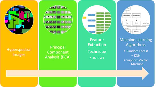
Figure 1 depicts the schematic representation of the proposed system. For this work, Indian Pines [29] and Salinas [30] airborne HSI datasets were used to experiment the proposed model. A hyperspectral image is a vector in high-dimensional space. The principal component analysis method (PCA) is used to reduce the subspaces in high dimensional data, producing computably compact image representation [31]. This represents all the pixels in an image using a new basis function along with the directions of maximum variation [26]. The DWT maps an image into other basis functions. These basis functions must have properties such as capture scale, invertible, orthogonal, square, pixel reduction, multi-scale representation, invertibility and linearity. Initially, the 1D-DWT is applied on the rows, and then, the output of 1D-DWT is fed along with the columns. This creates four sub-bands in the first stage of transformed space such as Low-Low (LL), LowHigh (LH), HighLow (HL) and HighHigh (HH) frequencies [32]. The LL band is equivalent to a downsampled (by a factor of two) version of the original image. Then, these features are applied to the random forest [33], KNN [33] and SVM [34] classifiers, and the results are compared with existing classification algorithm as decision tree, KNN and SVM without the use of the wavelet features.

3.1. Overview of DWT

In this section, we initially define the terminologies used in this paper and the procedure to extract feature from HSI images by using 3-dimensional discrete wavelet transform. Here, HSI data have X R ^ ( w * h * λ ) , where w and h are width and height of the HSI images, and λ is the wavelength or band of the entire HSI image spectrum. Here, input training samples are x = x 1 , x 2 , x 3 , x 4 x n R ^ ( b * n ) , where b is the translating function, and n should be less than w   and   h ,   y = y 1 , y 2 , y 3 , y n   K ^ n , where K is the number of classes. Wavelet transform is the best mathematical tool for performing time–frequency analysis and has a wider spectrum of applications in image compression and noise removal technique. The equation given below denotes the general wavelet transform
W f ( a , b ) = 1 a + x ( t ) φ * ( t b a ) d t  
where a is the scaling parameter, and b is the shifting parameter. φ(t) indicates the mother wavelet of the kernel function, and it is used to generate all the basic functions as prototypes. The translation parameter or the shifting parameter “b” gives the time information and location of the input signal. The scaling parameter “a” gives the frequency and detailed information of the input signal. DWT is given in Equation (3)
W p , q φ ( x ) = 1 a + x ( t ) a 0 p 2 φ ( t n b 0 a 0 p a 0 p ) d t  
where a 0 , b 0 are the dyadic scaling parameter and the shifting parameter, respectively. In multistage analysis, the signal x(t) will be recovered by the combination of different levels of wavelet and scaling function ( t ) and ψ ( t ) . Generally, Equation (3) can be rewritten for discrete signal x(n) as
x ( n ) = 1 M d C ψ [ i 0 , d ] ψ i 0 , d [ n ] + 1 M i = i 0 d D φ [ i , d ] φ i 0 , d [ n ]
where x ( n ) , ψ i 0 , d   [ n ] and φ i 0 , d [ n ] are discrete set functions that generally vary from [0, M−1], totally M points. Since ψ i 0 , d   [ n ] and φ i 0 , d   [ n ] are orthogonal to each other, the inner product can be obtained from the following wavelet coefficient equations
C ψ [ i 0 , d ] = 1 M n x ( n ) ψ i 0 , d [ n ]
D φ [ i , d ] = 1 M n x ( n ) φ i 0 , d [ n ]
In this work, we have used 3D-DWT feature extraction for hyperspectral images, which can be obtained from the expressions given in Equation (3) using different 1-D DWTs. This 3D-DWT generates several features with different scaling, orientations and frequencies. Haar wavelet is used as the mother wavelet in this work. The scaling and shifting functions are represented by the different filter bank (L, H) given by low-pass and high-pass filter coefficients l ( d ) and h ( d ) . Generally, Haar wavelet has l ( d ) = ( 1 2 , 1 2 ) and h ( d ) = ( 1 2 , 1 2 ) ; Fejér-Korovkin and Coiflet filters are used as wavelet filters in this paper and compared the same. Three-dimensional DWT is performed for hyperspectral imaging by expanding the standard 1-D wavelet to the image’s spectral and spatial domains, i.e., by applying the 1-D DWT filter banks in turn to each of the three dimensions (two for the spatial domain and one for the spectral direction). A tensor product is used to construct the 3-D DWT, which is shown in Equations (7) and (8).
X ( x , y , z ) = ( L x   H x ) ( L y   H y ) ( L z   H z )
X ( x , y , z ) = L x L y L z L x L y H z L x H y H z L x H y H z H x L y L z H x L y H z H x H y L z H x H y H z
where and denote the space direct sum and the product of the tensor, and X denotes the hyperspectral image, respectively. Figure 2 demonstrates the decomposition of 3D data into eight sub-bands after single-level decomposition implementation. The sub-band that has gone horizontally through the lowpass filter is called LLL in the vertical and spectral directions. This band is talking to data cube approximations. The vertex angle of the knowledge cube is seen by HHH band that went horizontally through the high-pass filter in vertical directions and spectral directions. The low- and high-pass filters along the x, y and z axes are expressed by L and H. The x and y directions, in practice, denote an image’s spatial coordinates, and the spectral axis is z. The volume data are broken down into eight sub-bands after single-level processing, i.e., LLL, LLH, LHL, LHH, HLH, HHL and HHH, which can be divided into three categories: approximation sub-bands (LLL), spectral variation (LLH, LHH, HLH) and spatial variation (LHL, HLL, HHL), respectively. At each scaling level, the convolution between the input and the corresponding low- or high-pass coefficients is performed. In the third stage of the filter bank, eight separate filtered hyperspectral cubes can be obtained. Then, these cubes again filtered with low-pass filter in all three dimensions to get the next level of wavelet coefficients, which is shown Figure 2. Here, this hyperspectral cube is decomposed into two levels, and it has 16 sub cubes ( U 1 , U 2 , U 3 , , U 15 ) as Equation (9).
x i , j = ( U 1 ( i , j ) , U 2 ( i , j ) , U 3 ( i , j ) , , U 15 ( i , j ) )
Consider the relationship between neighboring cubes to prevent edge blurring effects and lack of spatial information. The 3D wavelet features are derived from each local cube to integrate spatial and spectral information. In this work, the 3D wavelet coefficients of the entire cube are extracted after the first and second 3D-DWT levels. The LLL sub-band extracts the spatial information in the second-level 3D-DWT and the LLH band extracts the HSI data spectral information. The first and second stage knowledge vectors of all eight sub-bands are concatenated to make a vector with a size of 15 coefficients (removing approximate bands). It is called 3D data cube correlation, which helps to boost the compression. The basic concept is that a signal is viewed as a wavelet superposition. In comparison to 2D-DWT that decomposes only in horizontal and vertical dimensions, 3D-DWT has the advantage of decomposing volumetric date in horizontal, vertical and depth directions [35]. Three-dimensional DWT is performed for hyperspectral images by applying one-dimensional DWT filter banks to three spatio-spectral dimensions.

3.2. Hyperspectral Image Classification Using 3D-DWT Feature Extraction

The main objective of this work is to classify hyperspectral images using 3D DWT features. Random forest [36] is a classification algorithm that uses many decision trees models built on different sets of bootstrapped features. This algorithm will work with the following steps: Bootstrap the training set multiple times, the algorithm adopts a new set to build a single tree in the ensemble during each bootstrap. Whenever the sample of tree is split, a portion of features are selected randomly in the training sets for finding the best split variable and new features are evaluated. The random forest has taken more time to compute the process to validate the results, but its performance was good.
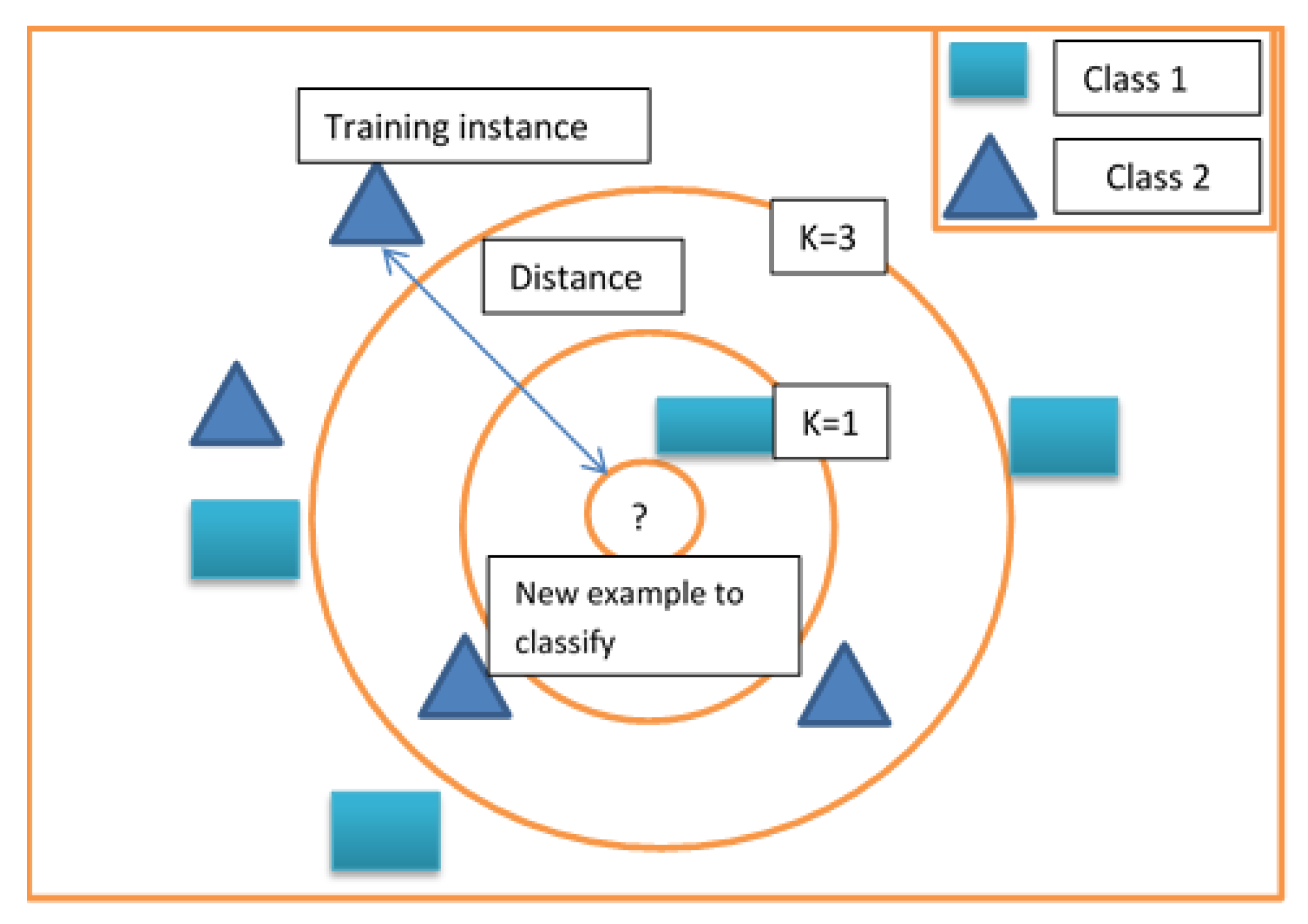
To overcome this issue, these algorithms are compared with KNN and SVM. K-nearest neighbors [KNN] is the second classifier adopted in the proposed method [36]. Given N training vectors, with “a” and “o” letters as input training features in this 2 dimensional feature space, this algorithm classifies the vector “c”, where “c” is another feature vector to be evaluated. In this case, it identifies the k-nearest neighbors regardless of labels. Consider the distribution of classes “a” and “o” as shown in Figure 3 with k equals 3. The aim of the algorithm is to find the class for “c”. Since k is 3, the three nearest neighbors of “c” must be identified. Among the three nearest neighbors, one belongs to class “a”, and the other two belong to class “o”. Hence, we have 2 votes for “o” and 1 vote for “a”. The “c” vector will be classified as class “o.” When k is equal to 1, the first nearest neighbor of the element will define the class. In KNN prediction, computation time is very slow, but training computation time is better than random forest. Even though training timing better compared to other algorithms, it requires more memory power to compute the HSI data. So, these algorithms are compared with SVM. This algorithm finds the most similar observation to the one we must predict and from which you derive a good intuition of the possible answer by averaging the neighboring values. The k-value, an integer number, is the neighbors that the algorithm must consider finding the solution. The smaller the k parameter, the more than the algorithm will adapt to the data we are using, risking overfitting but nicely fitting complex separating boundaries between classes. The larger the K-parameter, the more it abstracts from the ups and downs of real data, which derives nicely smoother carvers between classes in data. In KNN prediction, computation time is very slow but training computation time is better than random forest. Even though training timing is better than other algorithms, it requires more memory power to compute the HSI data. So, these algorithms are compared with SVM.
The SVM [32] model is a supervised learning method that looks at data and sorts it into one of the two categories. For example, in binary classification, SVM starts with a perception formulation and enforces certain constraints that are trying to obtain the separate line according to certain rules. This algorithm divides samples with the help of feature space using a hyperplane. Equation (8) will help to frame the SVM classification part
y ( x T w + b ) M
where x , w   and b indicate the input feature vector, weight vector and bias, respectively, and y is the predicted class. It provides a single value whose sign is indicative of the class, because y can be only −1 or +1 and may be equal or more than zero when the operations between parentheses have guessed the same sign as y. In the preceding expression, M is the constraint representing the margin. It is positive and the largest possible value to assure the best separation of predicted classes. The weakness of SVM is the optimization process. Since the classes are seldom linearly separable, it may not be possible for all the labels of training images to force the distance to equal or exceed constraint M. In Equation (10), the epsilon parameter is an optimization parameter for SVM, it allows us to handle with noisy or non-linearly separable data
y ( x T w + b ) M ( 1 + ϵ i )
The epsilon (ϵ) value will be zero for correctly classified classes. If the values of epsilon are between 0 and 1, the classification is correct, but the points fall within the margin. If the epsilon value is greater than 1, it means misclassification occurs, and it may be in the wrong side of the separating hyperplane. The general flowchart of 3D-DWT-based feature extraction and machine-learning classification is shown in Figure 4.
Algorithm 1: 3D-DWT-based feature extraction for hyperspectral image classifications
Input: Airborne hyperspectral image data XR^(w*h*λ), K is the number of classes.
Output: Predicted labels y.
  • The input feature vector X is converted into 3D-DWT features, UR^(w*h*15).
  • A certain amount of input features is selected for training randomly and remaining samples are used as ϵ testing samples.
  • The KNN, SVM, random forest machine-learning algorithm are trained using training samples.
  • The labels for testing samples are computed using all the machine-learning algorithms.

4. Results and Discussions

In this work, our proposed 3D-DWT-random forest, 3D-DWT-KNN and 3D-DWT-SVM methods are validated for two standard datasets such as Salinas Scene and Indian Pines hyperspectral data [37]. The results are compared with the same classifiers but without using information from the DWT. All coding required for this research has been carried out using MATLAB 2020b on a personal computer with 4GHz CPU and 8GB RAM. All the above mentioned algorithms are compared analytically using overall accuracy (OA), average accuracy (AA) and kappa coefficient [38]. Generally, OA gives the information about the number of correctly classified samples divided by the total number of samples. AA provides information about average accuracies of individual classes, whereas kappa coefficient (κ) indicates the two errors (omission and commission) and overall accuracy performance of the classifier. A confusion matrix as shown in Equation (12) is utilized to calculate the performance metrices.
C o n f u s i o n   m a t r i x   ( H ) = | H 11     H 12 H 1 K H K 1     H K 2 H K K |    
where H i j indicates the number of pixels, here “i” denotes the actual class, “j” denotes the predicted class and K indicates the total number of classes. The OA equation is shown in Equation (13).
OA = 1 N t e s t _ s a m p l e s i = 1 K H i i
where N t e s t _ s a m p l e s   is the total number of testing samples. The average accuracy is computed as shown in Equations (14) and (15).
C A i = H i i N i
AA = 1 K i = 0 K C A i
where N i is the total test samples in class i , and it varies from 0   t o   K . The kappa coefficient can be calculated by
κ = OA P e 1 P e    
where p e = i = 1 K ( P . i * P i . )   is the projected agreement, P i . = R i   N t e s t _ s a m p l e s ,   P . i = C i N t e s t _ s a m p l e s , R i   and   C i represent the summation of ith row and ith column in confusion matrix, respectively. Higher values of OA, AA and κ are expected by a good classifying algorithm.

4.1. 3D-DWT-Based Hyperspectral Image Classification Using Indian Pines Data

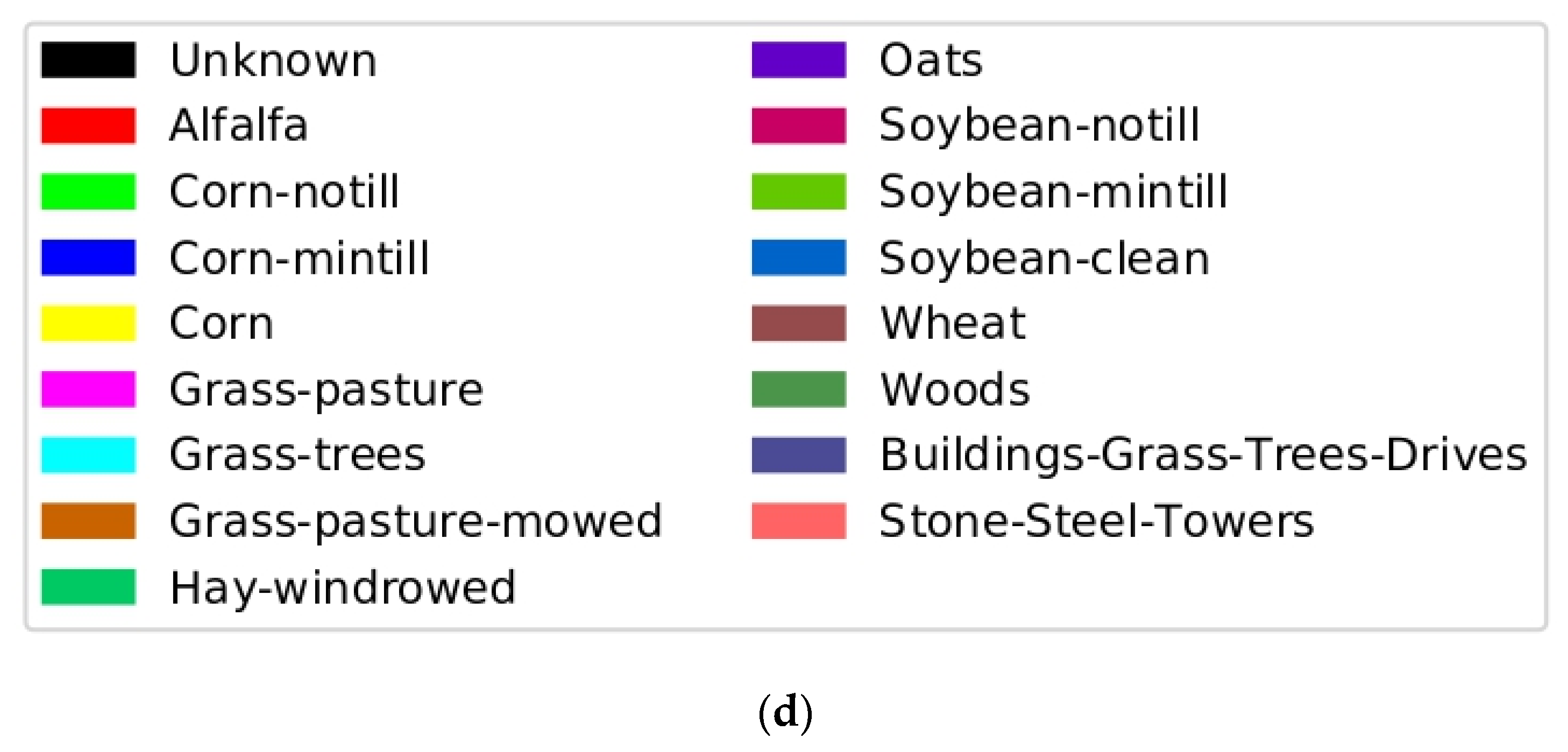
The Indian Pines dataset was collected by an airborne visible/infrared imaging spectrometer (AVIRIS) sensor. This dataset has been taken in North-West part of India in the year 1992. Each sample has 224 spectral bands with the spatial dimension of size 145 * 145 with ground truth data as shown in Figure 5. It includes 16 different vegetation classes, as shown in Table 1.
Initially, the 3D-DWT+random forest method is evaluated with labeled samples that have 60% data as training and 40% of data as testing samples. Principal component analysis (PCA) [39] is used to reduce the number of feature parameters to 15, to extract the significant information. the parameters considered in this work are (i) gamma value and (ii) epsilon value, which are tuned up to boost the performance of the proposed experiment. All the machine-learning algorithms were validated by K-cross validation (K = 10). Splitting the training dataset into k folds is part of the k-fold cross-validation process. The first k−1 folds are used to train a model, while the remaining kth fold serves as a test range. In each fold, we can use a variant of k-fold cross-validation that maintains the imbalanced class distribution. It is known as stratified k-fold cross-validation, and it ensures that the class distribution in each split of the data is consistent with the distribution of the entire training dataset. It also emphasizes the importance of using stratified k-fold cross-validation of imbalanced datasets to maintain the class distribution in the train and test sets for each model evaluation. In SVM, kernel function with 3rd order polynomial were used. Classification results of all the methods on Indian Pines dataset are shown in Figure 6, and the overall accuracy, average accuracy and kappa coefficients are reported and compared in Table 2. The best obtained results are highlighted in Table 2. Three-dimensional DWT+SVM performs better in terms of all performance metrices and larger improvement in this scenario; 3D-DWT+KNN and 3D-DWT+decision tree trail somewhat behind (79.4 and 76.2% OA, respectively). As shown in Table 1, 12,602 training samples from the Indian Pines data are selected. The overall accuracy of 3D-DWT+SVM is 88.3%, which is 14.5% larger than that of traditional SVM (77.1%). The classification maps of 3D-DWT+SVM are more closely related to the ground truth map. The observed results lead to misclassification due to the consideration of only spatial information, which can be rectified by including both spectral and spatial information. Wavelet coefficients from eight sub-bands capture the variations in the respective dimensions by implementing 3D-DWT over spatial–spectral dimensions. The local 3D-DWT structure is represented in three ways by the energy of the wavelet coefficients.
The confusion matrix for 3D-DWT + SVM in Indian Pines hyperspectral data is shown in Figure 7. The hyperspectral image classification outputs obtained by all the methods have more salt and pepper noise. This is because only spectral information is considered in both KNN and random forest methods. When both spectral and spatial information of Indian Pines hyperspectral data are used, it results in better OA. For a better understanding for calculating AA the steps are as follows: A sample calculation for computing AA is given as follows, for we consider true class Label 2, the total number of test sample of class 2 is 571, the predicted output of SVM of class 2 is 512, so the AA = 512 571 = 89.6 %   , which is shown in Table 2 (third row fourth column). In a similar way, we evaluated all the average accuracy of each class. Table 3 shows the OA, AA and kappa coefficient of entire class with different algorithms with help of Equation (14).
The proposed 3D-DWT features-based classifiers perform better compared to existing algorithms. The overall accuracy of test data is achieved SVM (77.1%), KNN (60.2%), random forest (67.7%), 3D-DWT+KNN (79.4%) and 3D-DWT+random Forest (76.2%) are less than the 3D-DWT+SVM method’s (88.3%) relative accuracy by 14.5, 46.7, 30.4, 11.2 and 15.9%, respectively. Table 3 discussed the comparison of adaptive weighting feature fusion (AWFF) with generative adversarial network (GAN) [40], and our proposed method of 3D-DWT-based KNN and SVM based on our test dataset. In this Table 3, we can say our proposed method has some improvement in terms of accuracy of individual classes because both spatial and spectral information are extracted to improve the performance of the classifications. Only few classes of AWFF-GANs have achieved more accuracies compared to our proposed method.
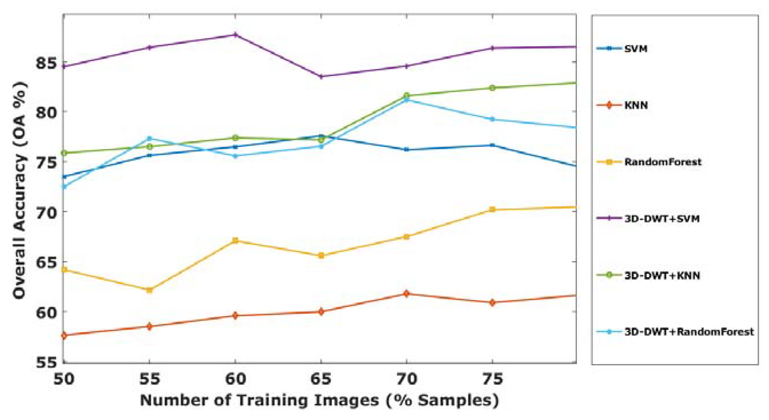
Initially 60:40 ratios are used for training and testing. Later, the effectiveness of our proposed method is evaluated with different number of training samples such as 50, 55, 60, 65, 70, 75 and 80% of supervised samples of each class from the Indian Pines HSI dataset. The overall accuracy for different training ratio is shown in Figure 8. The plot shows that out of several approaches proposed, the 3D-DWT+SVM achieves better performance in all aspects. Meanwhile, 3D-DWT+KNN and 3D-DWT+random forest obtain the second and third highest OA.

4.2. 3D-DWT-Based Hyperspectral Image Classification Using Salinas Scene Hyperspectral Data

The Salinas Scene dataset was collected by AVIRIS Sensor. This dataset was taken in Salinas Valley, California in the year 1998. These data have 224 spectral bands with the size of 512*217 spatial dimension with ground truth data and have 17 different landcover classes as given in Table 4. All the machine-learning algorithms were validated by K-cross validation. In SVM, kernel function with 3rd order polynomial were used.
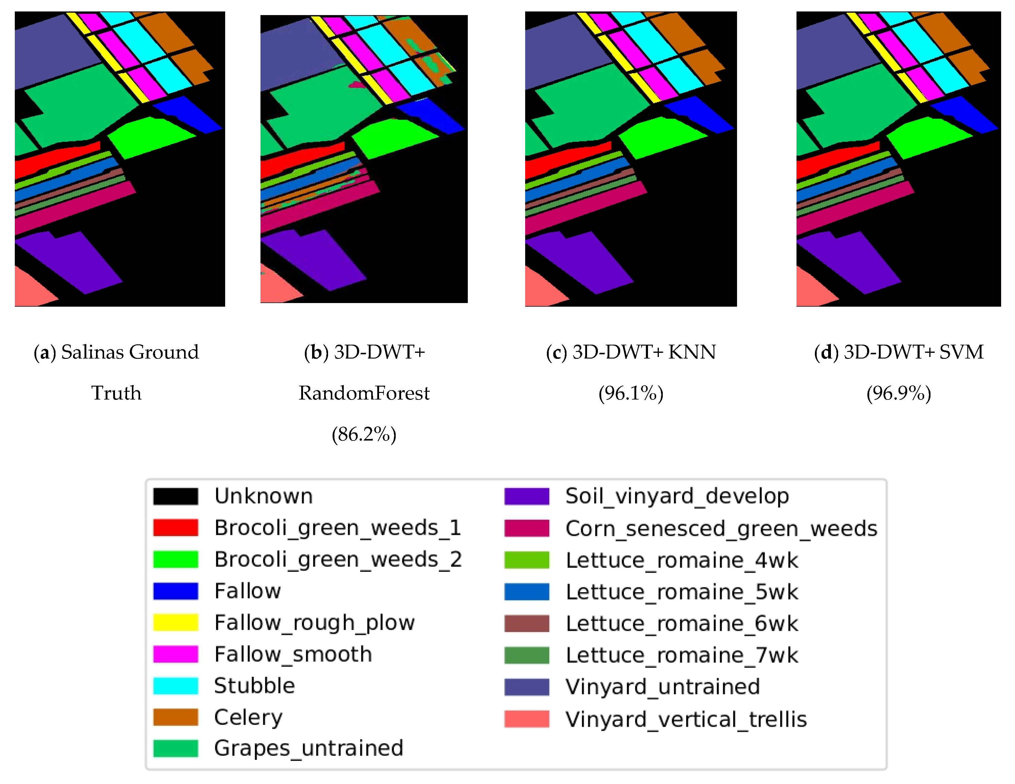
The confusion matrix (3D-DWT+SVM) for Salinas hyperspectral data is shown in Figure 9. Classification results of all the challenging methods on the ground truth of Salinas Scene hyperspectral data are shown in Figure 10. The overall accuracy, average accuracy and kappa coefficients of test datasets are reported and compared in Table 5. For a better understanding for calculating AA, the steps are as follows: A sample calculation for computing average accuracy is as follows, for we consider, true class Label 2, the total number of test sample of class 2 is 3725, the predicted output of 3D-DWT + SVM (Fejer-Korovkin filters) of class 2 is 3699, so the AA = 3725 3699 = 99.3 %   , which is shown in Table 5 (third row thirteenth column). In a similar way, we evaluated every average accuracy of each class. Table 6 shows the OA, AA and kappa coefficient of entire class with different algorithms with help of Equation (14).
From Figure 11 and Table 4, one and two best accuracies are highlighted: 3D-DWT+SVM performs better in terms of all performance metrices and larger improvement in this scenario; 3D-DWT+KNN and 3D-DWT+decision tree trail behind 3D-DWT+SVM with 96.1 and 86.2% OA, respectively [41]. Table 3 shows that 159,206 samples from Salinas Scene hyperspectral dataset were selected for training. The overall accuracy of 3D-DWT+SVM is 96.9%, which is about relative accuracy 7.54% larger than that of traditional SVM (90.1%). The classification maps of 3D-DWT+SVM is more closely related to the ground truth map.
The hyperspectral image classification output is obtained by all the computing methods. Three-dimensional DWT performs better than other methods, which is evident from the overall accuracy values. The OAs of SVM is 90.1%, KNN is 88.2%, random forest is 84.2%, 3D-DWT+KNN is 96.1% and 3D-DWT+random Forest is 76.2%.
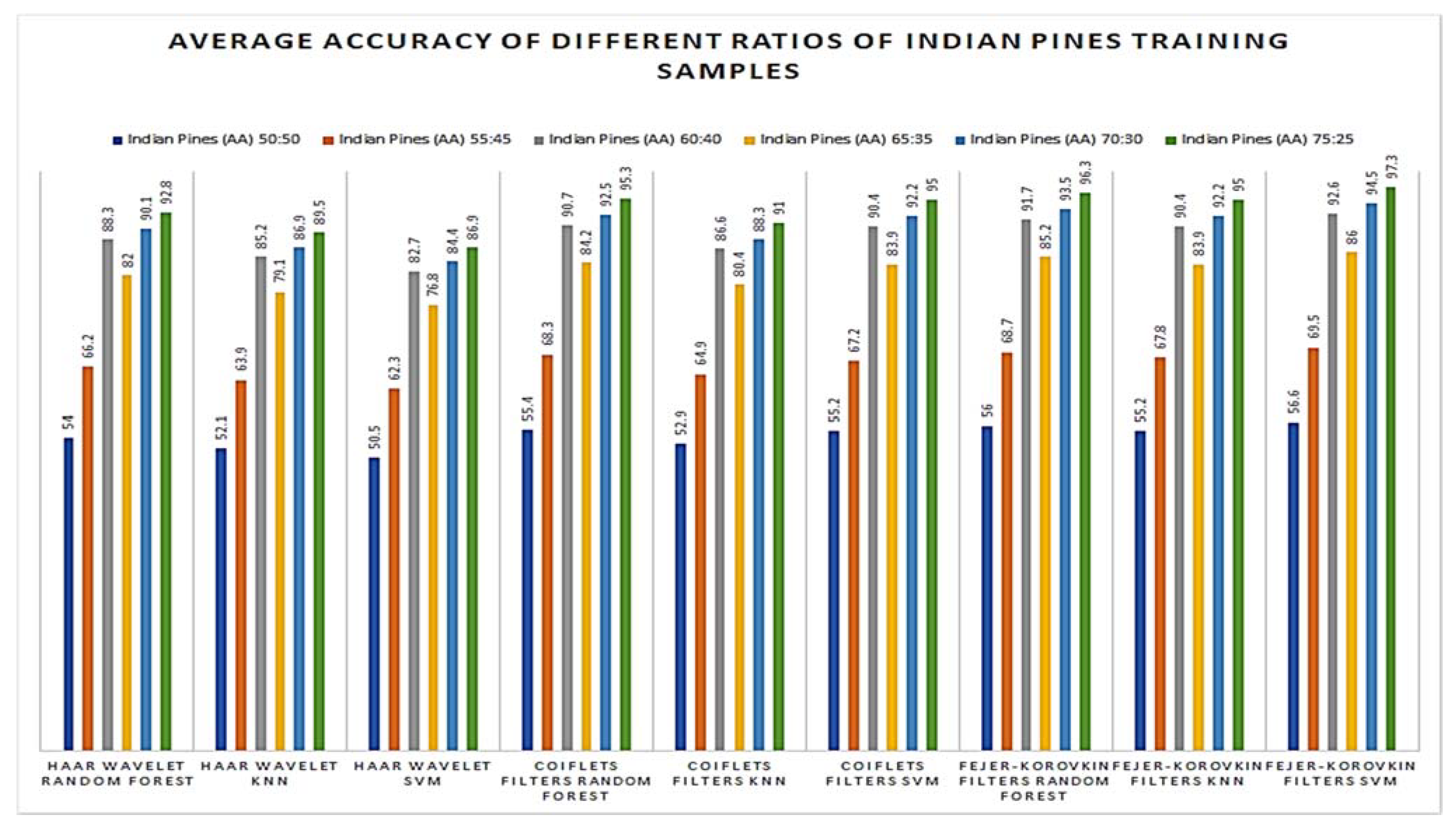
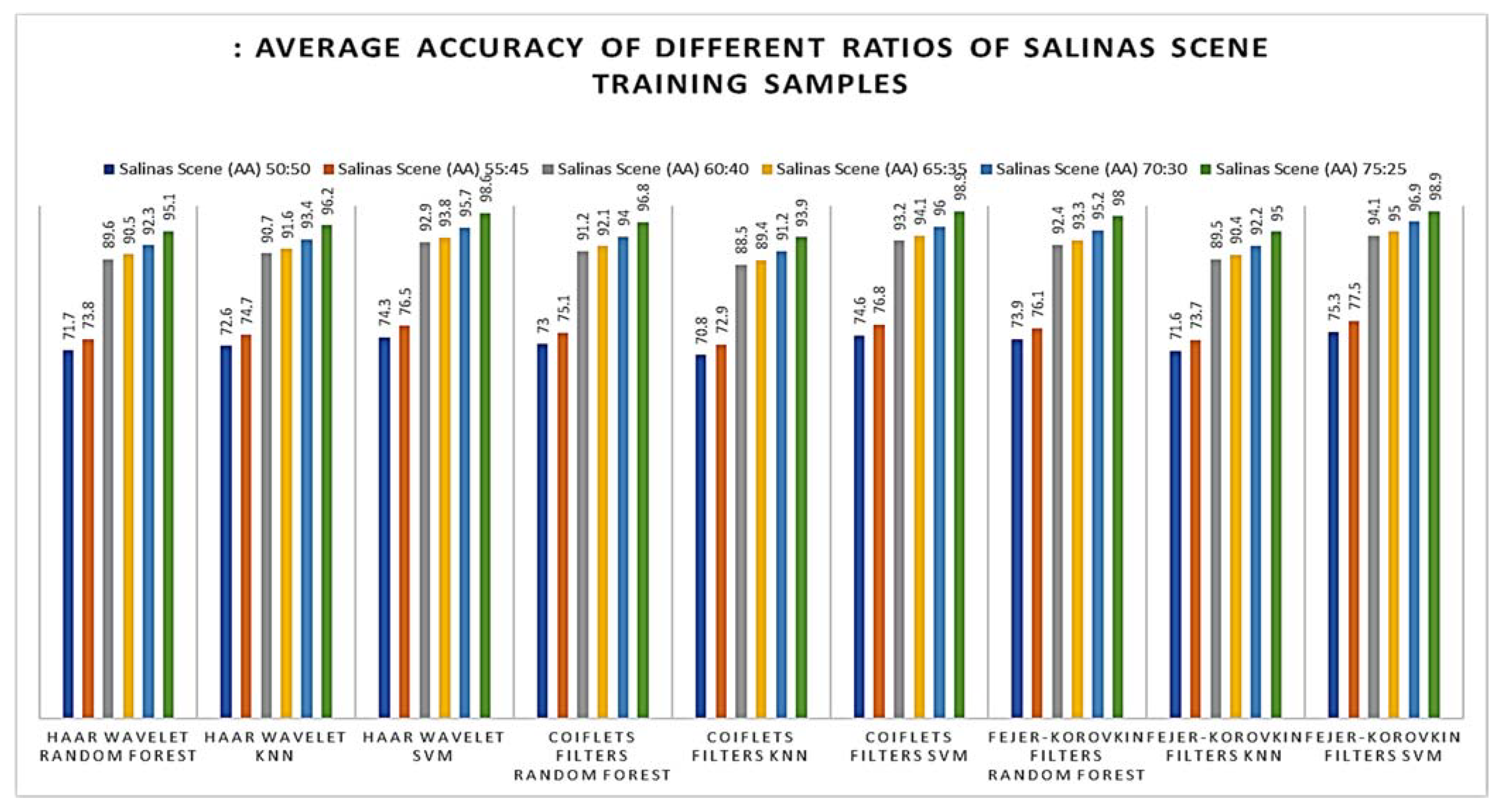
Later, the effectiveness of our proposed method was evaluated with different number of training samples such as 50, 55, 60, 65, 70, 75 and 80% of supervised samples of each class from the Salinas Scene hyperspectral dataset. The OA of different training samples are shown in Figure 11; from this, it is observed that the proposed method of 3D-DWT+SVM achieves better performance in all aspects. Meanwhile, 3D-DWT+KNN and 3D-DWT+random forest obtain the second and third highest OA. The computation time taken for training and testing datasets for our proposed method are as follows: the training times of 3D-DWT and testing times is 4 to 6 times greater than SVM, KNN and random forest, because it has both spatial and spectral features and a number of object prediction (testing data) in terms of seconds also shown in the Table 7. Figure 12 and Figure 13 show the average accuracy for a different ratio of training and testing images of Indian Pines (50:50, 55:45, 60:40, 65:35, 70:30, 75:25) and Salinas Scene (50:50, 55:45, 60:40, 65:35, 70:30, 75:25), respectively. In this, if we are increasing the number of training samples, increasing average accuracy of each class because both are directly proportional. From the analysis of Figure 11, if we are varying a different ratio of training and testing samples, the overall accuracy is not varying that much because of the unbalanced dataset.

5. Conclusions

In this work, a method of classifying hyperspectral image datasets is proposed by integrating spatial and spectral features of the input images. Based on the performance metrics such as overall accuracy, average accuracy and kappa coefficient, 3D-DWT+SVM achieves better performance in all aspects and has shown significant improvement in the results compared to the state-of-the-art techniques. Meanwhile, 3D-DWT+KNN and 3D-DWT+random forest attain the second and third highest OA for both widely used hyperspectral image datasets such as Indian Pines and Salinas. As a result, the intrinsic characteristics of 3D-DWT+SVM can be effectively represented to improve the discrimination of spectral features for HSI classification. The comparison of different ratio of training and testing images are providing a sufficient information about average accuracy of each class. Our future research will concentrate on how to efficiently represent spatial–spectral data and increase computational performance with the help of deep-learning algorithms.

Author Contributions

R.A. is responsible for the research ideas, overall work, the experiments, and writing of this paper. J.A. provided guidance and modified the paper. S.V. is the research group leader who provided general guidance during the research and approved this paper. All authors have read and agreed to the published version of the manuscript.

Funding

This research received no external funding.

Institutional Review Board Statement

Not applicable.

Informed Consent Statement

Not applicable.

Data Availability Statement

Not applicable.

Conflicts of Interest

The authors declare no conflict of interest.

References

  1. Elmasry, G.; Sun, D.-W. Principles of hyperspectral imaging technology. In Hyperspectral Imaging for Food Quality Analysis and Control; Academic Press: Cambridge, MA, USA, 2010; pp. 3–43. [Google Scholar]
  2. Gupta, N.; Voloshinov, V. Hyperspectral imager, from ultraviolet to visible, with a KDP acousto-optic tunable filter. Appl. Opt. 2004, 43, 2752–2759. [Google Scholar] [CrossRef]
  3. Vainshtein, L.A. Electromagnetic Waves; Izdatel’stvo Radio i Sviaz’: Moscow, Russian, 1988; 440 p. (In Russian) [Google Scholar]
  4. Engel, J.M.; Chakravarthy, B.L.N.; Rothwell, D.; Chavan, A. SEEQ™ MCT wearable sensor performance correlated to skin irritation and temperature. In Proceedings of the 2015 37th Annual International Conference of the IEEE Engineering in Medicine and Biology Society (EMBC), Milan, Italy, 25–29 August 2015; pp. 2030–2033. [Google Scholar]
  5. Shen, S.C. Comparison and competition between MCT and QW structure material for use in IR detectors. Microelectron. J. 1994, 25, 713–739. [Google Scholar] [CrossRef]
  6. Bowker, D.E. Spectral Reflectances of Natural Targets for Use in Remote Sensing Studies; NASA: Washington, DC, USA, 1985; Volume 1139.
  7. Chang, C.-I. Hyperspectral Imaging: Techniques for Spectral Detection and Classification; Springer Science & Business Media: Berlin/Heidelberg, Germany, 2003; Volume 1. [Google Scholar]
  8. Martin, M.E.; Wabuyele, M.B.; Chen, K.; Kasili, P.; Panjehpour, M.; Phan, M.; Overholt, B.; Cunningham, G.; Wilson, D.; Denovo, R.C.; et al. Development of an advanced hyperspectral imaging (HSI) system with applications for cancer detection. Ann. Biomed. Eng. 2006, 34, 1061–1068. [Google Scholar] [CrossRef] [PubMed]
  9. Huang, W.; Lamb, D.W.; Niu, Z.; Zhang, Y.; Liu, L.; Wang, J. Identification of yellow rust in wheat using in-situ spectral reflectance measurements and airborne hyperspectral imaging. Precis. Agric. 2007, 8, 187–197. [Google Scholar] [CrossRef]
  10. Wang, Y.; Duan, H. Classification of hyperspectral images by SVM using a composite kernel by employing spectral, spatial and hierarchical structure information. Remote. Sens. 2018, 10, 441. [Google Scholar] [CrossRef]
  11. Marconcini, M.; Camps-Valls, G.; Bruzzone, L. A composite semi supervised SVM for classification of hyperspectral images. IEEE Geosci. Remote. Sens. Lett. 2009, 6, 234–238. [Google Scholar] [CrossRef]
  12. Jian, Y.; Chu, D.; Zhang, L.; Xu, Y.; Yang, J. Sparse representation classifier steered discriminative projection with applications to face recognition. IEEE Trans. Neural Netw. Learn. Syst. 2013, 24, 1023–1035. [Google Scholar]
  13. Li, Z.; Zhou, W.-D.; Chang, P.-C.; Liu, J.; Yan, Z.; Wang, T.; Li, F. Kernel sparse representation-based classifier. IEEE Trans. Signal Process. 2011, 60, 1684–1695. [Google Scholar] [CrossRef]
  14. Hongyan, Z.; Li, J.; Huang, Y.; Zhang, L. A nonlocal weighted joint sparse representation classification method for hyperspectral imagery. IEEE J. Sel. Top. Appl. Earth Obs. Remote Sens. 2013, 7, 2056–2065. [Google Scholar] [CrossRef]
  15. Xiangyong, C.; Xu, L.; Meng, D.; Zhao, Q.; Xu, Z. Integration of 3-dimensional discrete wavelet transform and Markov random field for hyperspectral image classification. Neurocomputing 2017, 226, 90–100. [Google Scholar]
  16. Jun, L.; Bioucas-Dias, J.M.; Plaza, A. Spectral–spatial hyperspectral image segmentation using subspace multinomial logistic regression and Markov random fields. IEEE Trans. Geosci. Remote Sens. 2011, 50, 809–823. [Google Scholar]
  17. Youngmin, P.; Yang, H.S. Convolutional neural network based on an extreme learning machine for image classification. Neurocomputing 2019, 339, 66–76. [Google Scholar]
  18. Zhuyun, C.; Gryllias, K.; Li, W. Mechanical fault diagnosis using convolutional neural networks and extreme learning machine. Mech. Syst. Signal Process. 2019, 133, 106272. [Google Scholar]
  19. Zhenyu, Y.; Gao, F.; Xiong, Q.; Wang, J.; Huang, T.; Yang, E.; Zhou, H. A novel semi-supervised convolutional neural network method for synthetic aperture radar image recognition. Cogn. Comput. 2019, 1–12. [Google Scholar] [CrossRef]
  20. Zhengxia, Z.; Shi, Z. Hierarchical suppression method for hyperspectral target detection. IEEE Trans. Geosci. Remote Sens. 2015, 54, 330–342. [Google Scholar]
  21. Xudong, K.; Li, S.; Benediktsson, J.A. Spectral–spatial hyperspectral image classification with edge-preserving filtering. IEEE Trans. Geosci. Remote Sens. 2013, 52, 2666–2677. [Google Scholar]
  22. Akrem, S.; Abbes, A.B.; Barra, V.; Farah, I.R. Fused 3-D spectral-spatial deep neural networks and spectral clustering for hyperspectral image classification. Pattern Recognit. Lett. 2020, 138, 594–600. [Google Scholar]
  23. Zhang, X. Wavelet-Domain Hyperspectral Soil Texture Classification. Ph.D. Thesis, Mississippi State University, Starkvale, MS, USA, 2020. [Google Scholar]
  24. Wang, H.; Ye, G.; Tang, Z.; Tan, S.H.; Huang, S.; Fang, D.; Feng, Y.; Bian, L.; Wang, Z. Combining Graph-based Learning with Automated Data Collection for Code Vulnerability Detection. IEEE Trans. Inf. Forensics Secur. 2021, 16, 1943–1958. [Google Scholar] [CrossRef]
  25. Mubarakali, A.; Marina, N.; Hadzieva, E. Analysis of Feature Extraction Algorithm Using Two Dimensional Discrete Wavelet Transforms in Mammograms to Detect Microcalcifications. In Computational Vision and Bio-Inspired Computing: ICCVBIC 2019; Springer International Publishing: Cham, Switzerland, 2020; Volume 1108, p. 26. [Google Scholar]
  26. Shi, G.; Huang, H.; Wang, L. Unsupervised dimensionality reduction for hyperspectral imagery via local geometric structure feature learning. IEEE Geosci. Remote Sens. Lett. 2019, 17, 1425–1429. [Google Scholar] [CrossRef]
  27. Lei, J.; Fang, S.; Xie, W.; Li, Y.; Chang, C.I. Discriminative Reconstruction for Hyperspectral Anomaly Detection with Spectral Learning. IEEE Trans. Geosci. Remote Sens. 2020, 58, 7406–7417. [Google Scholar] [CrossRef]
  28. Luo, F.; Du, B.; Zhang, L.; Zhang, L.; Tao, D. Feature learning using spatial-spectral hypergraph discriminant analysis for hyperspectral image. IEEE Trans. Cybern. 2018, 49, 2406–2419. [Google Scholar] [CrossRef] [PubMed]
  29. Nagtode, S.A.; Bhakti, B.P.; Morey, P. Two dimensional discrete Wavelet transform and Probabilistic neural network used for brain tumor detection and classification. In Proceedings of the 2016 Fifth International Conference on Eco-friendly Computing and Communication Systems (ICECCS), Manipal, India, 8–9 December 2016; pp. 20–26. [Google Scholar]
  30. Aman, G.; Demirel, H. 3D discrete wavelet transform-based feature extraction for hyperspectral face recognition. IET Biom. 2017, 7, 49–55. [Google Scholar]
  31. Pedram, G.; Chen, Y.; Zhu, X.X. A self-improving convolution neural network for the classification of hyperspectral data. IEEE Geosci. Remote Sens. Lett. 2016, 13, 1537–1541. [Google Scholar]
  32. Gao, H.; Lin, S.; Yang, Y.; Li, C.; Yang, M. Convolution neural network based on two-dimensional spectrum for hyperspectral image classification. J. Sens. 2018, 2018, 1–13. [Google Scholar] [CrossRef] [Green Version]
  33. Slimani, I.; Zaarane, A.; Hamdoun, A.; Issam, A. Traffic surveillance system for vehicle detection using discrete wavelet transform. Transform, detection using discrete wavelet. J. Theor. Appl. Inf. Technol. 2018, 96, 5905–5917. [Google Scholar]
  34. Alickovic, E.; Kevric, J.; Subasi, A. Performance evaluation of empirical mode decomposition, discrete wavelet transform, and wavelet packed decomposition for automated epileptic seizure detection and prediction. Biomed. Signal Process. Control. 2018, 39, 94–102. [Google Scholar] [CrossRef]
  35. Bhushan, D.B.; Sowmya, V.; Manikandan, M.S.; Soman, K.P. An effective pre-processing algorithm for detecting noisy spectral bands in hyperspectral imagery. In Proceedings of the 2011 International symposium on ocean electronics, Kochi, India, 16–18 November 2011; pp. 34–39. [Google Scholar]
  36. Vinayakumar, R.; Soman, K.P.; Poornachandran, P.; Akarsh, S.; Elhoseny, M. Improved DGA domain names detection and categorization using deep learning architectures with classical machine learning algorithms. In Cybersecurity and Secure Information Systems; Springer: Cham, Switzerland, 2019; pp. 161–192. [Google Scholar]
  37. Anand, R.; Veni, S.; Aravinth, J. Big data challenges in airborne hyperspectral image for urban landuse classification. In Proceedings of the 2017 International Conference on Advances in Computing, Communications, and Informatics (ICACCI), Manipal, India, 13–16 September 2017; pp. 1808–1814. [Google Scholar]
  38. Prabhakar, T.N.; Xavier, G.; Geetha, P.; Soman, K.P. Spatial preprocessing based multinomial logistic regression for hyperspectral image classification. Proc. Comput. Sci. 2015, 46, 1817–1826. [Google Scholar] [CrossRef] [Green Version]
  39. Morais, C.L.M.; Martin-Hirsch, P.L.; Martin, F.L. A three-dimensional principal component analysis approach for exploratory analysis of hyperspectral data: Identification of ovarian cancer samples based on Raman micro spectroscopy imaging of blood plasma. Analyst 2019, 144, 2312–2319. [Google Scholar] [CrossRef]
  40. Liang, H.; Bao, W.; Shen, X. Adaptive Weighting Feature Fusion Approach Based on Generative Adversarial Network for Hyperspectral Image Classification. Remote Sens. 2021, 13, 198. [Google Scholar] [CrossRef]
  41. Luo, F.; Zhang, L.; Du, B.; Zhang, L. Dimensionality reduction with enhanced hybrid-graph discriminant learning for hyperspectral image classification. IEEE Trans. Geosci. Remote Sens. 2020, 58, 5336–5353. [Google Scholar] [CrossRef]
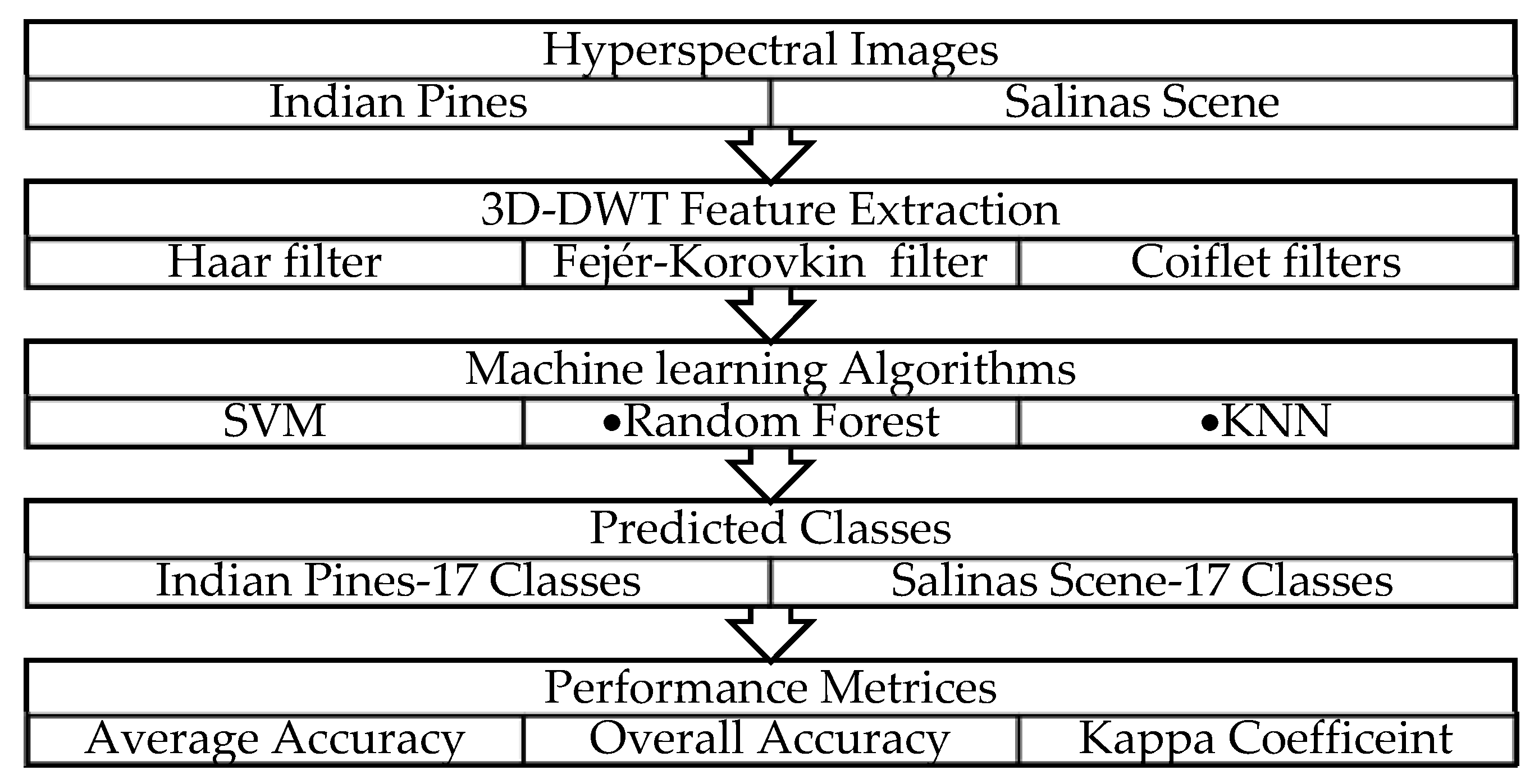
Figure 1. Schematic representation of proposed hyperspectral data processing flow.
Remotesensing 13 01255 g001
Figure 2. Three-dimensional DWT flowchart.
Remotesensing 13 01255 g002
Figure 3. Example of K-nearest neighbors (KNN).
Remotesensing 13 01255 g003
Figure 4. Machine-learning Algorithm 1 workflow.
Remotesensing 13 01255 g004
Figure 5. Indian Pines hyperspectral image: (a) Original Indian Pines data cube (145*145*224). (b) The Indian Pines ground truth image. (c) The training region of interest (ROI). (d) The classification legend for different classes.
Remotesensing 13 01255 g005aRemotesensing 13 01255 g005b
Figure 6. Classification output maps obtained by all computing methods on Indian Pines hyperspectral data (OA are described in parentheses).
Remotesensing 13 01255 g006
Figure 7. Confusion matrix for SVM in Indian Pines hyperspectral data.
Remotesensing 13 01255 g007
Figure 8. OA of all computing methods with different percentage of Indian Pines training samples.
Remotesensing 13 01255 g008
Figure 9. Confusion matrix for 3D-DWT+SVM (Fejer-Korovkin filters) in Salinas hyperspectral data.
Remotesensing 13 01255 g009
Figure 10. Classification output maps obtained by all computing methods on Salinas Scene hyperspectral data (OAs are described in parentheses).
Remotesensing 13 01255 g010
Figure 11. OA of all computing methods with a different percentage of Salinas Scene training samples.
Remotesensing 13 01255 g011
Figure 12. Average accuracy of different ratios of Indian Pines training samples (plot of different types of training and testing samples).
Remotesensing 13 01255 g012
Figure 13. Average accuracy of different ratios of Salinas Scene training samples (plot of different types of training and testing samples).
Remotesensing 13 01255 g013
Table 1. Indian Pines hyperspectral dataset.
Indian Pines ClassesTraining DatasetTesting Dataset
Label 0 Background 64654310
Label 1 Alfalfa2719
Label 2 Corn-no till857571
Label 3 Corn-min till486333
Label 4 Corn14294
Label 5 Grass-pasture290194
Label 6 Grass-trees438292
Label 7 Grass-pasture-mowed1711
Label 8 Hay-windrowed287191
Label 9 Oats128
Label 10 Soybean-no till583389
Label 11 Soybean-min till1473982
Label 12 Soybean-clean356237
Label 13 Wheat12382
Label 14 Woods759506
Label 15 Buildings-Grass-Trees-Drives232154
Label 16 Stone-Steel-Towers5637
Total12,6028411
Table 2. Classification accuracy of all the computing methods in Indian Pines dataset.
ClassRandom ForestKNNSVMAWFF-GAN3D-DWT+ Random Forest3D-DWT+KNN3D-DWT+SVM
Haar FiltersCoiflets FiltersFejer-Korovkin FiltersHaar FiltersCoiflets FiltersFejer-Korovkin FiltersHaar FiltersCoiflets FiltersFejer-Korovkin Filters
079.779.693.610085.486.086.191.692.192.291.191.691.2
193.866.789.598.0010010010094.484.210010068.493.3
270.956.689.690.1790.689.692.087.986.290.291.891.493.1
378.463.490.794.191.291.191.090.388.690.993.889.094.5
462.155.986.292.692.592.590.588.988.284.793.195.296.6
591.386.791.292.492.796.897.094.694.597.895.295.197.3
685.070.393.893.796.995.197.693.491.393.994.593.198.6
787.571.471.498.610085.790.090.981.890.910063.6100
889.577.696.296.991.495.293.494.094.592.796.897.396.9
910092.287.588.1100100100100100100100100100
1073.858.991.694.588.191.589.986.686.884.592.293.891.3
1176.869.394.292.692.190.391.991.090.390.293.193.193.0
1274.966.882.294.590.888.990.788.086.292.294.791.996.3
1391.578.891.597.996.197.296.297.497.494.098.798.896.4
1462.358.081.691.487.697.885.482.682.882.582.483.392.0
1550.051.168.088.197.897.491.491.591.085.489.783.891.2
1678.274.396.892.691.485.479.191.284.278.692.387.884.6
Table 3. OA, AA and kappa coefficient of entire class with different algorithms for Indian Pines hyperspectral data.
ClassRandom ForestKNNSVMAWFF-GAN3D-DWT+Random Forest3D-DWT+KNN3D-DWT+SVM
Haar FiltersCoiflets FiltersFejer-Korovkin FiltersHaar FiltersCoiflets FiltersFejer-Korovkin FiltersHaar FiltersCoiflets FiltersFejer-Korovkin Filters
Overall Accuracy (OA) 67.760.277.187.576.274.178.479.478.278.688.386.290.4
Average Accuracy (AA)72.166.489.690.888.385.282.790.786.690.491.790.492.6
Kappa Coefficient6.925.836.248.117.767.547.247.947.837.818.148.018.36
Table 4. Salinas Scene hyperspectral data.
Salinas Scene ClassesTraining DatasetTesting Dataset
Label 0 Background85,46356,975
Label 1 Brocoli green weeds 130142009
Label 2 Brocoli green weeds 255883725
Label 3 Fallow29641976
Label 4 Fallow rough plow20911394
Label 5 Fallow smooth40172678
Label 6 Stubble59393959
Label 7 Celery53693579
Label 8 Grapes untrained16,90711,271
Label 9 Soil Vinyard develop93056203
Label 10 Corn senesced green weeds49173278
Label 11 Lettuce romaine 4wk16021068
Label 12 Lettuce romaine 5wk28911927
Label 13 Lettuce romaine 6wk1374916
Label 14 Lettuce romaine 7wk16051070
Label 15 Vinyard untrained10,9027268
Label 16 Vinyard vertical trellis27111807
166,655111,103
Table 5. Classification accuracy of all the computing methods in Salinas Scene hyperspectral data.
ClassRandom ForestKNNSVM3D-DWT+Random Forest3D-DWT+KNN3D-DWT+SVM
Haar FiltersCoiflets FiltersFejer-Korovkin FiltersHaar FiltersCoiflets FiltersFejer-Korovkin FiltersHaar FiltersCoiflets FiltersFejer-Korovkin Filters
083.188.296.295.084.188.398.292.195.297.392.295.9
146.290.286.496.710092.295.392.110092.892.198.4
288.483.782.490.287.694.295.488.294.494.489.299.3
387.968.491.367.068.192.492.589.793.593.190.398.7
470.382.489.472.684.592.791.686.592.683.485.695.4
581.280.286.293.194.884.892.396.292.389.297.096.0
691.272.293.183.985.492.894.192.694.193.093.398.6
788.486.591.489.585.792.294.886.494.894.088.698.7
884.590.790.276.295.295.692.993.695.996.393.297.0
984.592.692.789.210010097.910094.996.610097.4
1087.590.292.652.862.372.196.885.6593.896.385.197.7
1183.387.588.595.692.190.793.790.392.790.790.296.5
1275.688.682.785.788.992.992.789.292.786.490.798.7
1382.286.288.697.896.998.492.095.792.492.894.994.8
1484.588.492.492.893.887.691.582.793.590.782.694.5
1586.585.290.289.790.293.691.488.292.489.886.895.7
1681.589.192.396.693.478.296.781.489.796.280.098.9
Table 6. OA, AA and kappa coefficient of entire class with different algorithms for Salinas Scene hyperspectral data.
ClassRandom ForestKNNSVM3D-DWT+Random Forest3D-DWT+KNN3D-DWT+SVM
Haar FiltersCoiflets FiltersFejer-Korovkin FiltersHaar FiltersCoiflets FiltersFejer-Korovkin FiltersHaar FiltersCoiflets FiltersFejer-Korovkin Filters
Overall Accuracy (OA)84.288.290.186.288.786.296.178.496.191.988.596.7
Average Accuracy (AA)86.690.292.489.690.792.991.288.593.292.489.597.1
Kappa Coefficient6.925.836.248.137.887.678.427.827.868.428.518.62
Table 7. Computation time of training phase and prediction speed of testing data.
AlgorithmsIndian PinesSalinas Scene
Training Time (Sec)Object Prediction Speed (Sec)Training TimeObject Prediction Speed (Sec)
Haar WaveletRandom Forest91.6800098.38000
KNN85.58410093.54100
SVM107.265000130.425000
Coiflets filtersRandom Forest88.03590095.425900
KNN86.3420092.664200
SVM104.854800110.354800
Fejer-Korovkin filtersRandom Forest103.458900113.548900
KNN82.824200101.234200
SVM118.885000142.475000
Publisher’s Note: MDPI stays neutral with regard to jurisdictional claims in published maps and institutional affiliations.