Article

Determination of Structural Characteristics of Old-Growth Forest in Ukraine Using Spaceborne LiDAR

by
Ben Spracklen
* and
Dominick V. Spracklen
School of Earth and Environment, University of Leeds, Leeds LS2 9JT, UK
*
Author to whom correspondence should be addressed.
Remote Sens. 2021, 13(7), 1233; https://doi.org/10.3390/rs13071233
Submission received: 23 February 2021 / Revised: 18 March 2021 / Accepted: 23 March 2021 / Published: 24 March 2021

Abstract

:
A forest’s structure changes as it progresses through developmental stages from establishment to old-growth forest. Therefore, the vertical structure of old-growth forests will differ from that of younger, managed forests. Free, publicly available spaceborne Laser Range and Detection (LiDAR) data designed for the determination of forest structure has recently become available through NASA’s General Ecosystem and Development Investigation (GEDI). We use this data to investigate the structure of some of the largest remaining old-growth forests in Europe in the Ukrainian Carpathian Mountains. We downloaded 18489 cloud-free shots in the old-growth forest (OGF) and 20398 shots in adjacent non-OGF areas during leaf-on, snow-free conditions. We found significant differences between OGF and non-OGF over a wide range of structural metrics. OGF was significantly more open, with a more complex vertical structure and thicker ground-layer vegetation. We used Random Forest classification on a range of GEDI-derived metrics to classify OGF shapefiles with an accuracy of 73%. Our work demonstrates the use of spaceborne LiDAR for the identification of old-growth forests.

Graphical Abstract

1. Introduction

There has been a noted growth of interest in the study of old-growth forests (OGF) over recent years and increased efforts to protect these areas. Human disturbance, including logging and deforestation for agriculture, has greatly reduced OGF occurrence and, in Europe, less than 1% of forest is classified as OGF or primary forest [1]. Valued for their carbon storage [2], biodiversity value [3], and beauty, these forests are characterised by a lack of detectable manmade disturbance and are generally noted for their abundant deadwood, trees of various ages and diameters resulting from natural regeneration, numerous large and old trees, and a complex canopy structure, consisting of multiple layers [4,5]. This presence of multiple vegetation layers is one of the key features that distinguishes OGF from younger stands, and can provide a useful means of classifying OGF.
The most common method of remotely studying forest is through the use of optical and radar sensors, such as the publicly available Landsat and Sentinel satellites. However, optical sensors provide limited information on forest structure, and while Synthetic Aperture Radar (SAR) sensors are perhaps better suited to the task, the 5.5 cm wavelength of the Sentinel-1 SAR satellite gives limited penetration of thick forest canopies [6]. Light Detection and Ranging (LiDAR) data, however, is better able to ascertain the forest canopy structure and is not so hampered by the signal saturation of optical and radar signals, with LiDAR beams able to penetrate the dense, multi-layered canopy. Given that OGF is characterised by a complex vertical structure, LiDAR seems strongly compatible with the remote study and classification of OGF. Additionally, forest structure provides important information on above-ground biomass storage, [7] biodiversity [8] and primary productivity [9].
Ground-based LiDAR studies of forest structure are common, with, for example, these recent papers [10,11,12,13] studying an OGF site in the Ukrainian Carpathians. Similarly, airborne LiDAR surveys of forest structure have become increasingly common over recent years. For example, there have been a number of studies of vertical temperate forest structure [14,15,16,17,18,19,20,21]. A Canadian study [22] used airborne LiDAR to estimate OGF attributes such as vertical complexity and understory density and developed an OGF index assessing the presence of characteristic features. However, due to operational costs ground and airborne studies are usually of limited areal extent. On the other hand, spaceborne LiDAR offers the potential for forest mapping on a global extent, but, to date, spaceborne LiDAR studies of forest structures [23] are fewer in number, and the potential has not been fully exploited. The Geoscience Laser Altimeter System (GLAS) on board the Ice, Cloud, and Land Elevation Satellite (ICESat) [24] acquired data between 2003 and 2009 that has been used to examine global forest canopy height [25,26] and aboveground biomass [27], but this instrument was optimised more to the study of polar icecaps than forest structure.
NASA’s General Ecosystem Dynamics Investigation (GEDI) [28] is a full-waveform, large-footprint LiDAR sensor mounted on the International Space Station, which began taking measurements between latitudes 51.6° N and S in March 2019. It is designed to provide high-resolution observations of forest vertical structure. Here we use this free, publicly available spaceborne LiDAR data to test the following hypotheses:
(1)
OGF will differ significantly from reference managed forest stands (non-OGF, NOGF) on a number of vertical structure metrics. We expect OGF to have a more open canopy and to be structurally more complex.
(2)
The differences in structure between OGF and NOGF will permit the effective use of Random Forest classification to classify OGF and NOGF.

2. Material and Methods
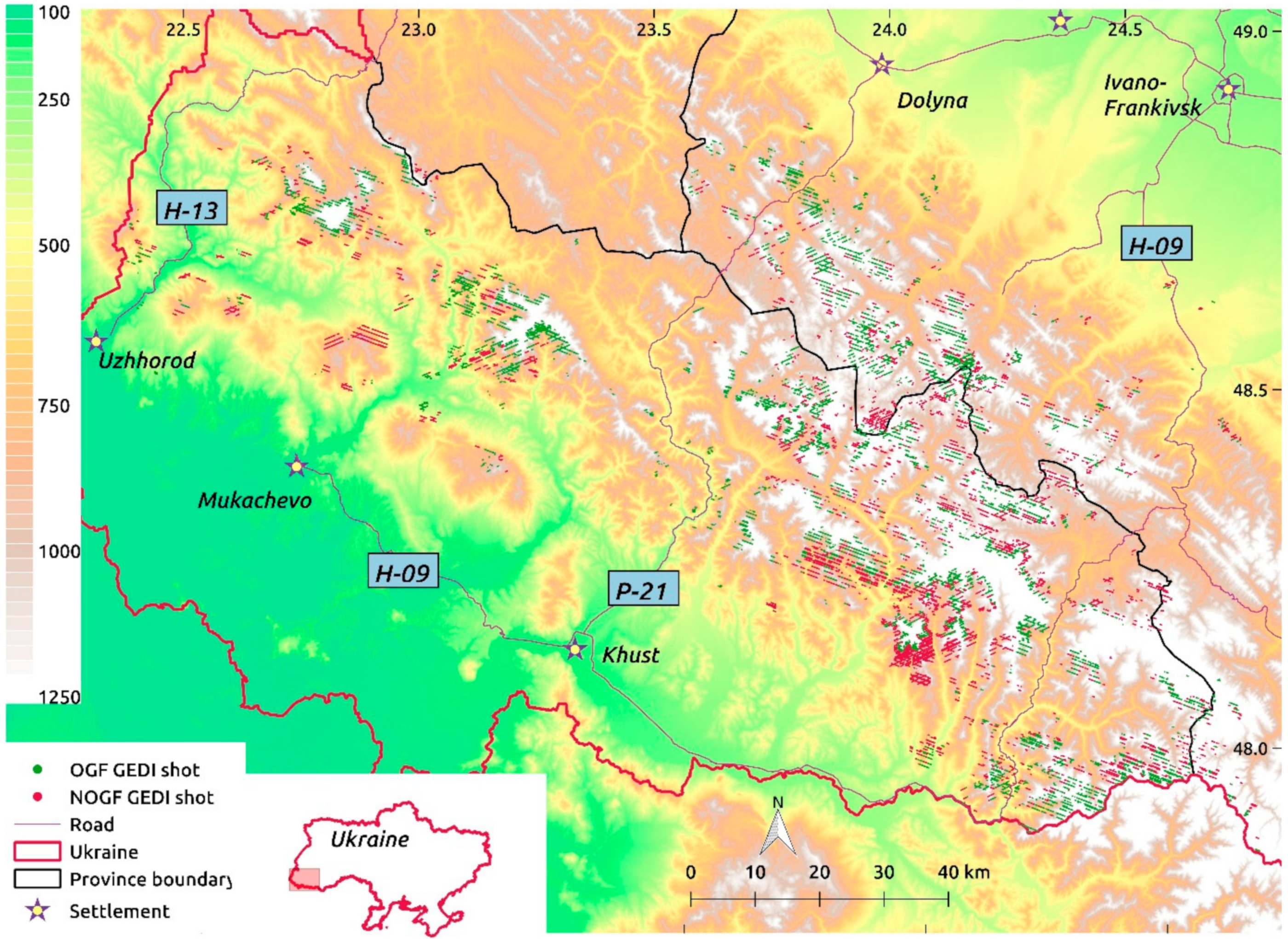
2.1. Study Area

The study was conducted in the Carpathian Mountains in the South-West of Ukraine, where there are still tens of thousands of hectares of high-quality OGF, including the largest contiguous forest of old-growth beech (Fagus sylvatica L.) in the world [29]. The remoteness of the mountains, the constant changing of historical borders, preservation as royal hunting grounds and distance from sufficiently large rivers to enable efficient timber extraction saved many areas from timber exploitation [30].
Forests in the Ukrainian Carpathians have recently been field-surveyed by the World Wildlife Fund (WWF) to identify any remaining areas of OGF [31]. Resulting from this survey were shapefiles of identified OGF, with each shapefile including detailed information on its tree species composition. Criteria used in the survey for identification of forest as OGF included abundant lying and standing deadwood, a complex structure with a high diversity of tree sizes and ages, and a lack of visible anthropogenic influence. All the stands in our study were surveyed between 2010 and 2018.
The surveyed OGF stands were largely single-species stands of beech, Norway spruce (Picea abies (L.) H. Karst) and Mountain pine (Pinus mugo Turra), with a limited occurrence of other species, such as sycamore maple (Acer pseudoplatanus L.) and silver fir (Abies alba Mill) alongside beech, and silver fir and stone pine (Pinus pinea L.) alongside spruce. The forest on the south-western side of the study area was dominated by beech, with a larger number of Norway spruce and mountain pine stands further to the east. Characteristically, the remnant OGF stands encircled open ground on the mountain tops, with managed forest occurring further down the mountain slopes. However, there were a number of lower-elevation OGF stands. For higher elevations, there was a change to scrub woodland or krumholz [32], with this forest type reaching as high as 1800 m in places. Krumholz largely consisted of mountain pine, with much smaller areas of green alder (Alnus alnobetula (Ehrh.) K.Koch), and was generally just a few metres tall. As the structure and height of this woodland type was completely different from the lower elevation OGF we excluded krumholz forest from our study, and we removed all mountain pine and green alder areas, and all areas with an elevation of over 1500 m.
The study area covered the province of Transcarpathia and the southern border of Ivano-Frankivsk province, containing 65,600 ha of OGF. Figure 1 shows the study area, with the location of GEDI shots used in this paper. All the WWF field survey data is available on the website http://gis-wwf.com.ua accessed on 23 March 2021 The OGF in this region is described in detail in a recent paper [33].
For comparative purposes, we selected Non-OGF shapefiles. These NOGF shapefiles had been surveyed by the WWF but had not met the criteria for classification as old-growth. The GEDI shots lying within these shapefiles were used for comparison to the OGF. The selected NOGF shapefiles were mostly adjacent to the OGF shapefiles. However, because the OGF tended to be a high-altitude forest this meant that adjacent NOGF was usually lower in elevation. Therefore, we selected some high-elevation, tree-line adjacent NOGF shapefiles that lay further away from the OGF. We selected sufficient NOGF shapefiles so that the number of shots within OGF and NOGF areas was roughly equivalent.
NOGF areas have been primarily managed in a system of large-scale clear-felling and replanting, resulting in a forest of even-aged stands of plantation forest. In 2009 it was estimated that in the Ukrainian Carpathians, 72% of harvested timber derived from clear-felling, 24% shelter-belt cutting, and just 4% as a result of selection thinning [34]. While in recent years there has been an increased emphasis on sustainable forest management practices, [35] with the ultimate aim of producing more uneven-aged stand structures and continuous forest cover, much of the NOGF in the study area will be of an even-aged plantation structure, with a simplified age, species, and spatial structure.

2.2. GEDI

The GEDI LiDAR system is comprised of three lasers, with one of the lasers split into 2 beams, giving four tracks (see Figure 2). The three lasers are also dithered, producing a total of eight parallel tracks. Each track consists of approximately 25 m diameter footprints over which the 3D structure is measured by recording the amount of laser energy reflected at different heights above ground. The footprints of each track are separated by 60 m and the tracks themselves separated by about 600 m. The four tracks produced by the split laser beams are referred to as cover tracks and the other four tracks as power tracks. LiDAR noise will be least when the power beams are operating during the night, and greatest for the cover beams operating during the day [36]. The coverage and power beans are designed to be able to detect the ground through 95% and 98% canopy cover respectively [28]. Each GEDI shot is given a sensitivity value, which is the estimated maximum canopy cover that can be penetrated given the signal-to-noise ratio of the waveform. For our study, the mean ± standard deviation sensitivity of the coverage beams was 0.947 ± 0.021 and for the power beams 0.969 ± 0.016.
The ground elevation of each GEDI shot (above sea-level) is produced by the GEDI’s LiDAR instrument. Additionally, the elevation given by the TanDEM-X digital elevation model is also provided in the GEDI products. TanDEM-X elevation values are produced using X-band Synthetic Aperture Radar (SAR) on two satellites, have a resolution of 0.4 arcseconds and in forested, mountainous terrain similar to our study area have a mean error of ±8–10 m [37,38].

2.3. GEDI Data Analysis Methods

To ensure that all the measurements were taken with the leaves fully out and without snow cover, we restricted GEDI measurements to between 1 June and 30 September. In Ukraine, the beech trees begin to leaf-out in mid-April at the lowest elevations, and by the start of June are all fully emerged. Each GEDI shot has a quality flag field, with a value of one indicating good quality. We discarded any measurements without a quality flag equal to 1.
The GEDI datasets used in this study are the L2A and L2B processing level, downloaded over the co-ordinates 48.9–47.4° N, 22.3–24.7° E from 2 June to 29 September 2019, and 2 June to 1 September 2020. We had a total of 18,489 ‘good-quality’ shots in OGF and 20,398 shots in NOGF. 48% of these were taken at night (solar elevation less than 0°).
After downloading, all the GEDI shots were converted to shapefile format. Using shapefiles of OGF and NOGF across the region, all the shots were classified as either OGF or NOGF. Further, both OGF and NOGF shots were then classified as either broadleaf, conifer or mixed conifer/broadleaf. Forest in this last category has a conifer proportion of between 20 to 80%.
Broadleaf forests in the study area were predominantly pure beech or beech dominated: of the 9113 shots in broadleaf, 8711 were in pure beech forest and 304 in a beech-dominated mix with another broadleaf species, principally sycamore. There were small areas of other broadleaved species: 75 shots in sessile oak (Quercus petraea (Matt.) Liebl), nine shots in ash (Fraxinus excelsior L.), and eight in hornbeam (Carpinus betulus L.) Similarly, conifer forests were dominated by Norway spruce. Of the 6152 conifer shots, 5435 were in pure Norway spruce forest and 522 in a Norway spruce-dominated mix with another conifer species, principally silver fir. There were just seven shots in scots pine (Pinus sylvestris L.), 16 in stone pine and 159 in silver fir. In other words, 99% of the OGF broadleaf category was either beech or a beech-dominated broadleaf mix, while 97% of the OGF conifer category was either Norway spruce or a Norway spruce-dominated conifer mix.
The principal part of the L2A product is 101 relative height metrics at 1% intervals (rhx with x from 0,1,2,…99,100). These are the percentiles of the vertical energy distribution in a returned waveform, with the values giving the height in metres above ground below which the specified percentage x of the LiDAR’s energy is returned. So for example, an rh80 value of 10 m would mean that 80% of the energy was reflected below height 10 m from the ground. The top value, rh100, is the height of the canopy top and rh0 the bottom of the ground signal. Note that the lowest rh height values are usually negative due to ground return, particularly where the canopy is sparse. We added a number of these relative height values into our model. Additionally, a number of metrics were computed from these relative height values (see Table 1.)
We calculated a foliage thickness curve by dividing each LiDAR shot into ten equal height strata, so that, for example, a 20 m canopy will be divided into ten 2 m strata, and a 5 m tall canopy divided into ten 0.5 m strata. The percentage of energy reflected from the ground to the canopy top (above-ground energy) by each of these strata is calculated, with the thickest canopy strata reflecting the most and the thinnest the least. The skewness and kurtosis of this curve were then computed. Kurtosis is a measure of the combined weight of the tails compared to the rest of the distribution, with a positive value indicating ‘tail-heavy’ distribution. Skewness is a measure of the symmetry of the distribution with positive values indicating a heavy tail on the right-hand side of the distribution, negative values a heavy tail on the left-hand side, and a value of 0 a symmetrical distribution.
We calculated the height of the thickest portion of the canopy, which will be the height at which there is the least change in adjacent rh height values (Thickest Canopy metric.) This metric was given as a fraction of canopy height (rh100.) The Vertical Height Distribution (VHD) [8] is a measure of the evenness of canopy distribution, with a thick top canopy and limited understory producing low values, and a more evenly distributed canopy having values approaching 1. We adapted this index as:
V H D = rh 100 rh m i d rh 100
where rh100 is the canopy height and rhmid is the height of the midpoint of the above-ground return. For example, if 60% of the energy is above-ground return, then the midpoint would be rh70.
A LiDAR study [10] in Central and Eastern Europe (including the Ukrainian Carpathians) of the difference in understory complexity of beech stands managed by thinning compared to unmanaged OGF found significant differences between the Ukrainian OGF study site and some of the managed sites, dependent on stand age and presence of tree regeneration. Hence we formulated a herb layer metric, calculated as the energy reflected by the herb layer, defined as being from the ground to 1 m tall. This metric was given as a fraction of energy reflected from the ground to the canopy top. Similarly, we also calculated the fraction of the above-ground energy reflected by the shrub layer, which we defined as being from 1–5 m tall (shrub metric.)
We used five values from the L2B product: the plant area index (PAI), the canopy cover, the Foliage Height Diversity (FHD), and the ground and canopy components of the waveform rg and rv (see Table 1). PAI describes the horizontal projected area of vegetation per unit of ground area (m2 m−2) within a volume of canopy. Canopy cover is defined as the per cent of the ground covered by the vertical projection of canopy material. The Foliage Height Diversity is a measure of canopy complexity and is calculated from the vertical distribution of the PAI:
F H D = i = 1 k p i × l n ( p i )
where pi is the proportion of PAI in vertical height bin i, with the L2B product binning the canopy into 5 m tall layers, and k is the total number of height bins. Higher fractions of PAI in a layer will give a smaller contribution to FHD so that lower values are associated with simple, single-layered canopies. The ground component is the integral of the waveform ground component. Likewise, the canopy component is the integral of the waveform vegetation component. We calculate the fractional ground return as
G r o u n d   r e t u r n = r g r g + r v
All the aforementioned L2A and L2B processing was done using Python. We noted forest structure differed between areas of shorter and taller canopies. Therefore, we examined canopy structure separately for canopy heights of less than and greater than 25 m. This specific value was chosen as it was roughly half the maximum canopy height, and has been used in European forest studies as the definition of the upper canopy layer [39], or to divide mature and middle-aged woodland from younger stands [40].

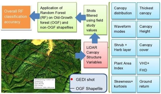
2.4. Random Forest Classification

We used the Random Forest (RF) method [41] to classify GEDI shots as either OGF or NOGF based on the metrics detailed in Table 1. RF is a non-parametric tree technique that has been widely used for both classification and regression in determining forest structural properties with airborne [21,42,43,44,45,46,47] and spaceborne [26,48,49,50] LiDAR. Additionally, a previous paper [51] that had looked at the classification of OGF and NOGF in Ukraine used optical Sentinel-2 imagery and RF Classification. To make this paper more comparable with that paper we also opted for using RF classification. RF works by generating numerous trees from a random subset of training data, and randomly selects predictor variables for use in each tree.
The classification analysis was performed using the scikit-learn Python library [52]. The number of trees built was set at 500 and the maximum number of features used in an individual tree was the square root of the total feature number. There was a slight excess of OGF shots to NOGF shots and so we randomly sampled the OGF shots to produce an equal number (using the ‘sample’ function in python Pandas, random_state = 1). We assess accuracy using the producer’s accuracy (how often actual features are correct), user’s accuracy (how often predicted features are correct) and total accuracy (correct predictions to total predictions made). Differences in classification accuracies were examined for significance using the 2-proportion Z-test, [53] which compares the proportions of correctly classified results. The result of the Z-test is reported as the χ2 value and associated p value, with a statistically significant level defined as 5%.
The classification analysis was carried out twice—firstly on each individual GEDI shot and then for OGF and NOGF shapefiles which contained more than one shot in their area. In the second case, we used the median value of the multiple shot values, and additionally, added the standard deviations of the indicated metrics in Table 1. In each case, the classification is carried out separately for conifer forests, broadleaf forests and mixed forests, with the results then combined and reported. However, we recognize that to run the RF classification separately on the different forest types requires detailed knowledge of the area, which is not always as readily available as it is in our study area. We therefore also carry out the RF classifications without separating the forest types and examine how this impacts the classification accuracy.

3. Results

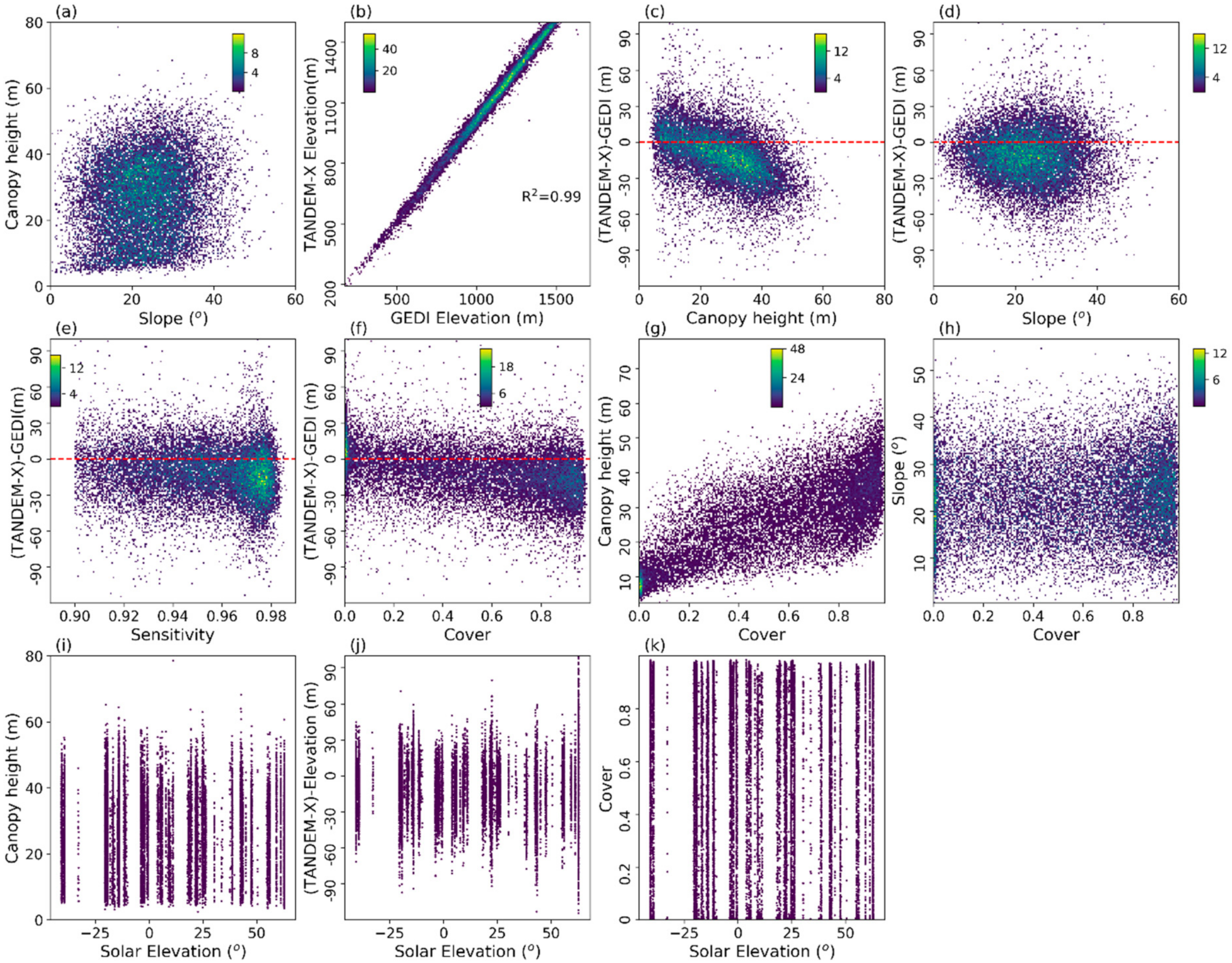
3.1. Erroneous Measurements

We noticed anomalous values of certain GEDI measurements. Figure 3 shows estimated canopy height, ground elevation, and canopy cover measurements as a function of different variables.

3.1.1. Erroneous Canopy Height Measurements

We found 2.4% (n = 224) of canopy height measurements in beech OGF were above 50 m, with the tallest at 64.4 m. Sources [29,54,55] suggest a maximum canopy height for beech in Ukraine of about 47–50 m. Studies in other European countries have found similar maximum heights: 53.7 m in Serbia [56], 51.7 m in Romania [57], and 49 m in Germany [58]. In mixed forests, Norway spruce and silver fir can grow several metres taller than beech [59]. However, visual analysis of winter Sentinel-2 (S-2) images of the area with anomalous canopy heights showed no signs of any conifer trees in the area. Following processing, the average geolocation error of the GEDI shots was estimated to be in the order of 10–20 m [28], roughly equivalent to 1–2 S-2 pixels.
For conifer OGF, 0.2% (n = 13) height measurements were over 53 m, with a maximum reading of 78.6 m. A field study [60] at elevations of 800–1200 m in the Ukrainian Carpathians suggested a maximum height value for Norway spruce of 53 m.
We used 1 arc-second Shuttle Radar Topography Mission (SRTM) [61] elevation data to calculate the slopes of all shots in the study. The average slope of all GEDI beech OGF shots was 23.5°, with 82% of shots at slopes of over 15°. The suspect maximum height values were, on average, on slightly steeper terrain, as the average slope of beech height values over 50 m was 27.4°. While there were a few suspect shots on flatter terrain, Figure 3a shows the majority at slopes of over 20°. However, removing shots based on slopes was not a viable option, as there were simply too few shots on flatter terrain.
There were considerably more suspiciously high canopy height readings in broadleaved than conifer woodland. Just 0.2% of conifer shots were over 53 m tall, compared to 1% of broadleaved shots. Suspect shots were taken both during night-time and day-time (Figure 3i). 59% of canopy height readings over 53 m were taken during the night-time.

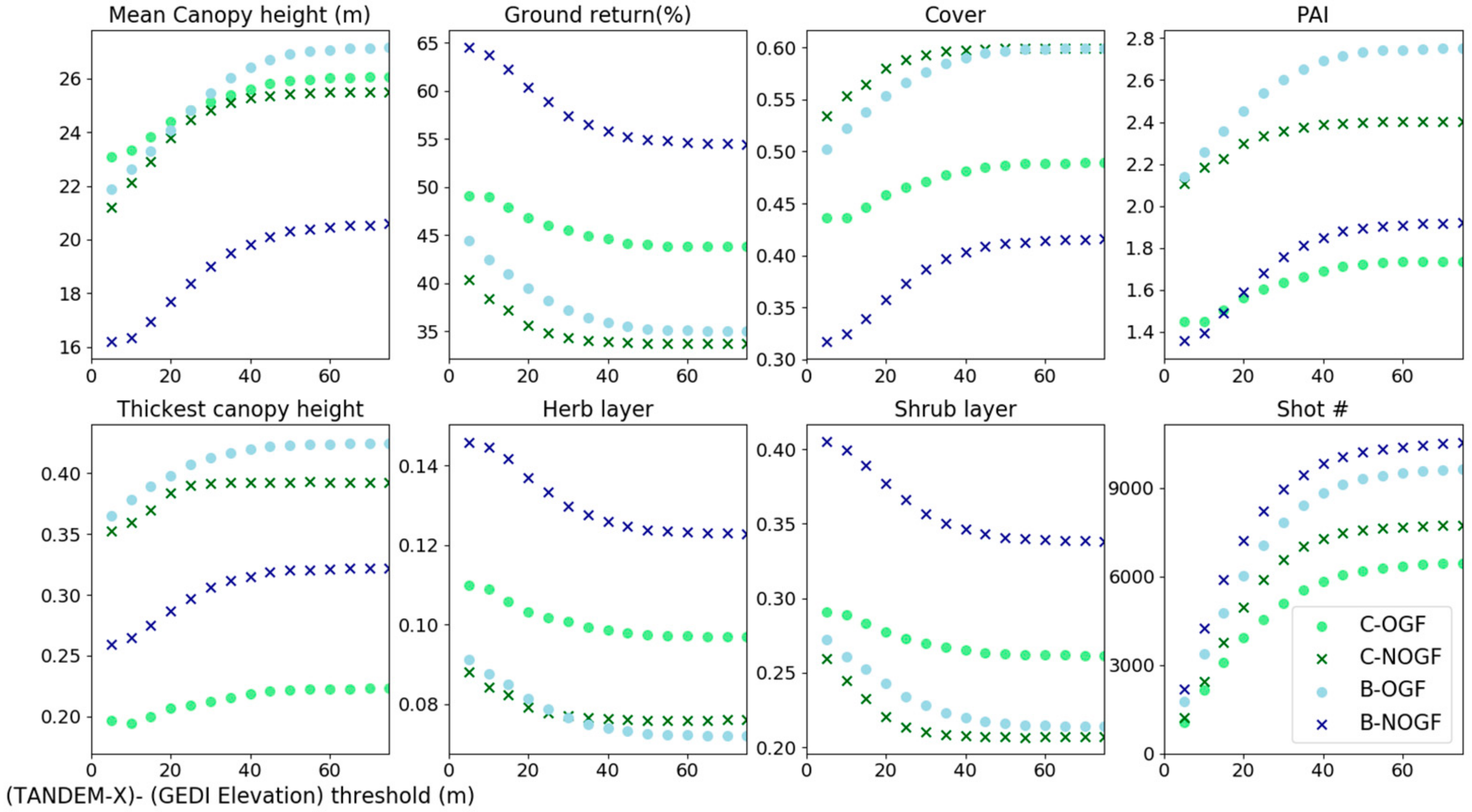
3.1.2. Erroneous Ground Elevation Measurements

The TanDEM-X and GEDI-derived ground elevation values were strongly correlated (R2 = 0.99, Figure 3b.) However, we noted a small number of extreme outliers where the ground elevation values given by the GEDI shot was significantly different from that given by TanDEM-X, with a maximum difference of 321 m (see Figure 3b.) The median difference between the two elevation values (TanDEM-X –GEDI) was −11.5 m, and the median absolute value 15.9 m.
Figure 3c shows an association between outlier canopy height readings and the TanDEM-GEDI elevation difference, with almost all the canopy heights over 50 m having overestimated GEDI elevation readings. In our study, high elevation differences tended to occur on the steeper terrain, with an average slope of 27.1° for an elevation difference of over 50 m and 29.4° for an elevation difference of over 100 m, compared to an average slope for all GEDI shots of 23.2° (see Figure 3d.)
Linear regression showed that sensitivity had a significant, but minor effect (p < 0.0001, R2 = 0.002) on the absolute elevation error readings (Figure 3e), with higher sensitivity associated with higher errors. Naively, we expected lower sensitivity values with outlier elevation difference values. We note that a previous study [36] found no change in elevation accuracy with GEDI sensitivity. Higher canopy cover was associated with higher absolute errors (p < 0.0001, R2 = 0.03) in the ground elevation readings (see Figure 3f.)
Erroneous elevation readings were strongly associated with a single track (rightmost track in Figure 3j)—the highest solar elevation in the study at 62.7–62.9°. The average absolute elevation error for this track was 43.8 m, compared to 19.1 m for all shots.
Figure 4 shows the impact on selected structural metrics of removing all shots with an absolute difference between the TanDEM-X value and the GEDI value above a given threshold value. The removal of shots had a similar effect on OGF and NOGF metrics. We regard the TanDEM-X elevation data as the accurate elevation dataset.

3.1.3. Erroneous Canopy Cover Measurements

A field study [62] in beech OGF in the Ukrainian Carpathians of 314 plots, each of an area of 0.05 ha and elevation ranging from 458 to 1269 m, found very thick canopy cover values, with almost 80% of plots with a canopy cover over 0.7, and only about 5% with a cover of less than 0.5. The minimum canopy cover was about 0.15. Another field study [54] in the Ukrainian Carpathians in five sites of beech OGF of elevation from 550–760 m found mean canopy covers of between 0.89–0.92. A study [60] of two Norway spruce OGF stands in the Ukrainian Carpathians found mean canopy closures of 0.81 and 0.93.
There was a mismatch between our canopy cover values and these aforementioned field studies. There were a very large number of shots with extremely low cover values (see Figure 3f–h). A total of 6.8% and 18.1% of OGF and NOGF shots have a cover of less than 0.05, these shots overwhelmingly having canopy height values of between 5–15 m (see Figure 3g). A visual examination in Google Earth and a Sentinel-2 RGB image from the 15 September 2020 of a sample of these shots confirmed they consisted of forest—that is, they were not clearings or harvested sites. These extremely low values occurred at a large range of TanDEM-GEDI elevation differences (Figure 3f), slope values (Figure 3h) and on all solar elevation tracks (Figure 3k.) They occurred much more often in broadleaf than conifer forests, with 12% and 31.3% of broadleaf OGF and NOGF having a cover under 0.05 respectively, compared to 5.7% and 6.8% of conifer OGF and NOGF. Figure 5 shows the impact on selected structural metrics of removing all shots with a canopy cover below a given threshold.

3.1.4. GEDI Shot Removal

Using the results of field studies in the Carpathian Mountains, we decided to remove all shots with canopy height values over 50 m for the broadleaved shots, and all shots with canopy height values over 53 m for conifer and mixed forest shots. This results in the removal of 277 (1.5% of total) and 176 (0.9% of total) OGF and NOGF shots respectively.
The relationship between faulty elevation readings and suspect canopy height shots means that shots that were inaccurate in elevation will be more likely to be inaccurate in terms of canopy height and possibly structure. However, we wanted to avoid removing lots of shots from our study if possible. We investigated removing all GEDI shots with (a) an elevation difference of 25 m (26% of total shots) and (b) 50 m (4% of total shots) from our study. We found that the use of these two different threshold values did not alter the statistical significance in the comparison of OGF and NOGF structural metrics. The change in RF classification accuracy was also small: 0.4% higher for the first case (a). Therefore, we decided to keep as many GEDI shots as possible, and only removed shots with an elevation difference of over 50 m from our study. This resulted in discarding 835 (4.5% of total) OGF and 714 (3.5% of total) NOGF GEDI shots.
Again using the results of Ukrainian Carpathian field studies, it was clear that many of the canopy cover values were too low. Again we were keen to keep as many shots as possible in our study. We investigated removing all GEDI shots with (a) a cover of less than 0.15 (22.5% of total shots) and (b) 0.45 (38.9% of total shots). These values are chosen based on field studies in Ukrainian beech OGF, with the former being the minimum canopy cover value found, and the latter the lowest canopy cover value at which a large number of measurements were found. RF classification accuracy was 0.4% higher in the first case (a). Therefore we again decided to keep as many GEDI shots as possible and removed any shots with a cover of less than 0.15.
In summary, we perform three filters of the GEDI shots: the removal of erroneous canopy height measurements, the removal of erroneous ground elevation measurements and the removal of erroneous canopy cover values. This resulted in the total removal of 3932 (20.3% of total) OGF and 6780 (32.7% of total) NOGF GEDI shots from the study, leaving us with 14,557 OGF and 13,618 NOGF shots for use in the remainder of the paper.

3.2. Forest Structure

3.2.1. Conifer Structure

Figure 6 compares canopy heights in OGF and NOGF. The mean ± standard error of the canopy height was 27.8 ± 0.1 m for conifer OGF (97% Norway spruce) compared to 27.5 ± 0.1 m for conifer NOGF. The maximum conifer OGF height detected was 52.5 m, at an elevation of 979 m. 0.3% (n = 16) of conifer data had a canopy height over 50 m.
Figure 7 shows the boxplots of selected structural metrics for OGF and NOGF. There was a significant difference between OGF and NOGF conifer structures on all tested metrics except Foliage Height Diversity and canopy height (see Table 2). Indeed, the overall maximum canopy height distribution was similar for OGF and NOGF (see Figure 6a). OGF was more open, with lower values of canopy cover and PAI, and higher values of ground return energy. Conifer OGF was marked by a thick herb and shrub layer compared to NOGF (see Table 2 and Figure 7).
Although the difference in canopy heights was minimal, there were substantial differences in canopy structure between OGF and NOGF conifer. Figure 8 shows the mean canopy thickness values over the 10 height strata. There was a significant difference between the height of the thickest canopy layer, which in conifer OGF was near the ground (about a tenth of canopy height), and in NOGF nearly seven-tenths canopy height. Conifer OGF had a thicker understory but a more even distribution of vegetation in the upper layers compared to NOGF. Both had an upper layer peak in the 60–70% height strata, but this peak was considerably more marked compared to the four layers below in NOGF than in OGF.

3.2.2. Broadleaf Structure

Broadleaf OGF was significantly different from NOGF on all selected metrics. However, if we restrict the analysis to tall forests (maximum canopy height over 25 m), OGF and NOGF are more similar. Neither had much in the way of ground cover, with much lower values of herb and shrub layer than for conifer forests. However, NOGF still had a significantly thicker canopy, with higher PAI and canopy cover and lower values of ground return (see Table 3). While for tall woodland, both categories had their thickest layer at over half canopy height, OGF beech was significantly more layered than NOGF, with a higher number of modes, and higher values of FHD and VHD.

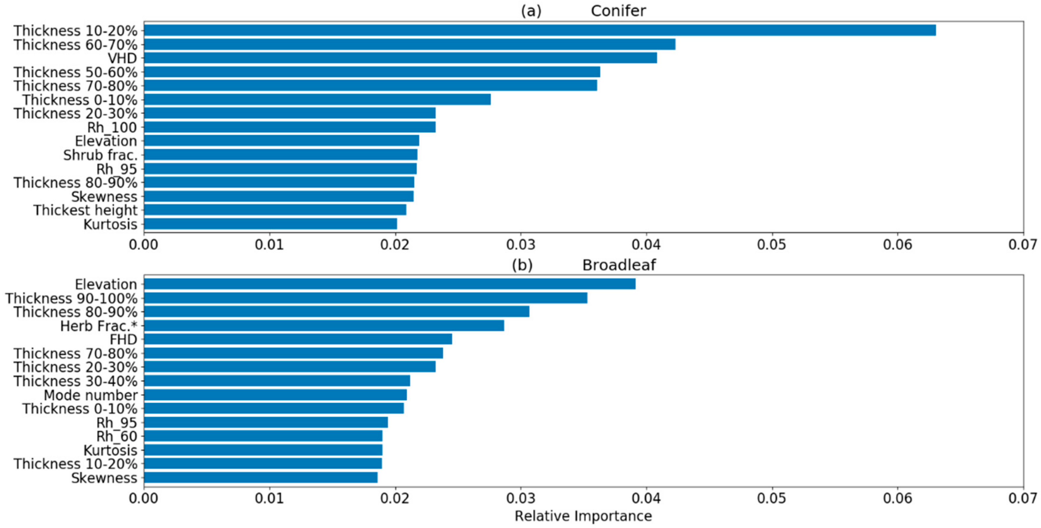
3.3. Random Forest Classification

Random Forest classification was done for both each individual GEDI shot (Table 4a) as well as for shapefiles that contained more than a single GEDI shot (Table 4b). In both cases, the classification for conifer, broadleaf and mixed forest was run separately, and then the results combined. The producer’s and user’s accuracies for the Random Forest classifications were reasonably equal, with all values between about 70 and 80%. There was a higher overall accuracy for shapefiles (Table 4b) than for individual GEDI shots (Table 4a), but the difference was not significant (2-proportion Z-test).
For individual shots, the overall accuracy in conifer forests (73.9%) was significantly higher (2-proportion Z-test, χ2 = 3.2, p = 0.001) than in broadleaf (70.5%). In turn, the overall accuracy in broadleaf was significantly higher (2-proportion Z-test, χ2 = 4.6, p < 0.001) than in mixed forest (63%). Running the RF classification on the conifer, broadleaf and mixed forest types as a mixture resulted in a significantly lower accuracy than in running the classification separately on the different forest types and then combining the results. For shapefiles, it resulted in a significantly lower (χ2 = 2.5, p = 0.01, 2-proportion Z-test) overall accuracy of 68.1%.
Figure 9 shows the most important features for the classification of shapefiles for conifer and broadleaf forests. The foliage thickness curves provided 7 of the top 15 features for both conifer and broadleaf. However, the most important features for conifer and broadleaf was generally quite different, with only 8 of the top 15 features in common. The standard deviation values of the metrics rated very poorly with only one appearance for broadleaf and none in conifer. However, it can be seen that there was no outstandingly important feature in either forest type.

4. Discussion

Large-waveform, remotely sensed LiDAR has encountered significant problems with producing accurate measurements on steeply sloped terrain in previous studies. The steeply sloped ground has been linked to erroneously high canopy height readings [36,66,67], with studies [36,67] suggesting that canopy height errors increase sharply above a slope of about 10–15°. Using GEDI data, a study [36] of temperate, mostly coniferous forest in Germany found a Mean Absolute Deviation (MAD) value of 5 m for slopes of 20–25° and 6 m for slopes greater than 25°. Canopy height error is worsened in areas of high canopy cover, [36] with increased difficulty in the LiDAR return accurately detecting the ground. For this reason, LIDAR is known to have higher accuracy in conifer than broadleaved forests [66,68,69], due to the latter’s more closed canopy in summer months (see Figure 7).
Similarly, rugged terrain is well known to cause LiDAR ground elevation reading problems [36,70,71,72]. A number of studies [71,72] have noted LiDAR elevation errors increasing sharply for slopes over 15–20°. The GEDI geolocation error can clearly lead to an error in a given height if the location error is in the same direction as the slope. For our study area, using our mean slope value of 23.2°, the extreme value of the GEDI geolocation error (horizontal error of 20 m) and assuming a constant slope value, the vertical error could be as high as 8.5 m. The thick forest canopy is also associated with greater inaccuracies in LiDAR elevation readings [71,73]. These errors can be particularly acute for thick forest canopy on sloped terrain [72]: the LiDAR ground returns are spread out over different heights, and ground and vegetation returns can occur at the same height, leading to difficulty in distinguishing the ground return in the reflected waveform. However, even taken in tandem, neither the impact of heavily sloped terrain and dense forest can really account for some of the extremely large difference values that we see.
The cause of extremely low canopy cover values is harder to explain, with them occurring on shallow slopes and for low values of elevation error. They occur more often in NOGF than OGF and more often in broadleaf than conifer forests. Interestingly, almost all these erroneous cover values had canopy height values of between 5–15 m, so filtering out the low cover values had no effect on our findings for canopies over 25 m tall.
One study, using spaceborne LiDAR [74], dealt with the problems caused by steep slopes by removing all LiDAR shots with a slope of over 10°. Such an approach in mountain forests such as those analysed here would leave us with insufficient data. However, the terrain of the two forest types in our study was fairly similar—the mean ± standard deviation slope of OGF and NOGF shots was 23.2 ± 8.5° and 21.2 ± 8.6° respectively. This means that any errors should be similar in both forest categories, and since we are interested in relative differences, rather than absolute values, this should hold less importance. Despite this we still filtered our GEDI readings, discarding any canopy height values over thresholds given by field studies from the study area. More significantly, we used the difference in GEDI-derived ground elevation and an independently SAR-produced ground elevation dataset as an indicator of reliability. Even more importantly, we employed a third filter by removing all values of canopy cover below 0.15, based on a study area field study. Together this resulted in us discarding about 25% of GEDI data, with a lower data discard amount in OGF compared to NOGF.
Both broadleaf and conifer OGF had a unimodal canopy top height distribution, with the peak at 25–30 m for spruce and 30–35 m for beech. In contrast, field studies [59,65] found bimodal distributions for both beech and spruce, with peaks at 15–20 m and 40–45 m for spruce and 5–10 m and 30–40 m for beech. We attribute the cause of this disagreement to the different output from large footprint GEDI and field studies. The former will record the height of the highest tree in a roughly circular, 25 m diameter area of approximately 0.05 ha. In contrast, field studies record the height of every tree within the plots, resulting in a larger variability in canopy heights.
In terms of structure, OGF is typically characterised by vertical complexity and horizontal heterogeneity [4]. On a horizontal level, OGF typically has canopy gaps and patches of dense tree regeneration. On a vertical level, OGF typically has multiple layers, or a continuous distribution of vegetation between the ground and canopy top, with the presence of sub-canopy layers comprised of suppressed mature trees, shrubs and regenerating tree saplings. In our study area, these characteristics were present in both conifer (predominantly Norway spruce) and broadleaf (predominantly beech) OGF (Figure 6, Figure 7 and Figure 8). Beech OGF had a ‘top-loaded’ vertical canopy distribution, with its thickest layer at about 60% of canopy height, while Norway spruce forest had its thickest layer much closer to ground level.
We find significantly smaller values of PAI and canopy cover in tall (>25 m canopy height) broadleaf OGF compared to NOGF. We expect lower canopy cover in beech OGF than younger woodland due to increased treefalls and deadwood. However, the absolute differences in these two metrics are much smaller than found between conifer OGF and NOGF. For tall beech stands, there was no significant difference in herb layer between OGF and NOGF, though the shrub layer was significantly thicker in OGF. These results are in agreement with a number of field studies [39,55] of virgin beech forests that have noted a sparse middle layer and understory, often described as a ‘hall’ or ‘cathedral’ type structure. In contrast, almost twice as much energy was reflected from the shrub layer in tall conifer OGF than NOGF, and above the lowest canopy thickness layer, the canopy distribution is notably more evenly distributed than for conifer NOGF, or both broadleaf forest categories. The lack of a significant difference in Foliage Height Diversity index between conifer OGF and NOGF, therefore, seems surprising, given that higher values of FHD are associated with more complex, multi-layered canopies. Figure 8, however, shows the very thick ground layer in conifer OGF which will be reducing the FHD value. Therefore, number of modes and the VHD index, both significantly higher in conifer OGF than NOGF, seem to better capture the canopy complexity than FHD.
Both Norway spruce [75] and beech [76] are considered to be shade-tolerant species that can withstand lengthy periods of slow growth under the forest canopy. However, at high elevations, Norway spruce’s shade tolerance is reduced, and semi-open spruce stands can be found [77]. We found conifer OGF was significantly more open, with a lower canopy cover compared to NOGF. Contrary to our results, a field study [60] of three Norway spruce—Silver fir stands in Ukraine, two old-growth and one managed—found no significant difference in canopy cover.
Due to the sampling nature of the GEDI project, it was harder to examine the horizontal structure of the forest. An individual GEDI shot covers a roughly circular area of about 20–25 m diameter, dependent on factors such as the slope of the ground, and so covers an area of about 300–500 m2. For both conifer and broadleaf, only 1% of shots had a canopy height under 10 m tall (see Figure 6). Large footprint LiDAR can have a challenging time accurately measuring the height of short-statured vegetation [78,79], especially on steeply sloping terrain. However, field studies in the Carpathians have tended to find numerous, fine-scale canopy gaps in beech [80,81,82], beech-fir [83], and beech-fir-spruce [84,85] old-growth forest, but very few gaps larger than 500 m2, consistent with our results.
Our analysis shows spaceborne LiDAR can be used to classify OGF, with an accuracy of 71–73%. A similar study [22] in a forest in Canada used Random Forest and airborne LiDAR to classify OGF from younger stands, using the following metrics: canopy cover, vertical complexity, 90% canopy height, understory density and, as an ancillary feature, Wetness Index. Understory density was found to be the most important feature and OGF was classified with an accuracy of about 60%. In the same area of the Ukrainian Carpathians as our study, a paper [51] classified OGF from NOGF using optical Sentinel-2 data and Random Forest, with a classification accuracy of shapefiles of 85%.
The current sparse sampling density of GEDI—with only 53% (3225 of 6014) of OGF shapefiles in the study area currently having any quality shots, and 7% (431) having just one shot—is currently a drawback to the use of GEDI. The use of multiple shots to classify a shapefile allows the use of metrics such as the standard deviation of values which are useful for classification purposes. The sampling should become denser as more GEDI data becomes available in the future, likely increasing classification accuracy.
Contrariwise, the optical S-2 sensor provides information from all over the shapefile at a resolution of 10–20 m, probably producing the higher classification accuracies seen with that sensor. The possibility of boosting classification accuracies through the integration of Sentinel or Landsat optical data with GEDI data is an interesting area of further study.
Historically, management of forest in the Ukrainian Carpathians has largely consisted of clear-felling and replanting, with minimal interest in continuous cover forestry. This practice generally results in blocks of even-aged plantation forests. A ground-based LiDAR study [11] has noted that the structural complexity of continuous cover forestry is significantly greater than in even-aged monocultures. Therefore, we note that distinguishing OGF from forests managed over long periods of time with continuous cover precepts may prove to be a tougher proposition than in areas like our study site where plantation forestry is the predominant management practise. Such difficulties and differences may prove an interesting avenue of research.
Despite the challenges encountered in using LiDAR on such difficult terrain, we believe the use of GEDI shows promise in the determination of vertical structure in complex temperate forests. This can not only prove useful in identifying potential old-growth stands, but over time could be used to track the development of old-growth characteristics in mature forests. More widely, these methods could be used for evaluating a woodland’s importance for biodiversity: the species diversity of birds, for example, is greater in taller, more complex forests with a higher number of layers [86]. Similarly, mammal diversity has been shown to be positively related to LiDAR-derived structural complexity, and negatively related to cover [87]. Forest structure also has a strong control on the speed at which fire spreads through a forest, with structurally complex forests decreasing fire spread [88]. Further work is required to explore whether the structural complexity of OGF provides any protection from forest fires.

5. Conclusions

The difficulties inherent in ground and airborne LiDAR have restricted the determination of the vertical stand structure of old-growth forest to small plots or areas. Here we use GEDI—a spaceborne LiDAR system—to investigate the vertical structure of old-growth beech and spruce forest over tens of thousands of hectares of the Carpathian Mountains of western Ukraine. From a LiDAR perspective, the Ukrainian Carpathian Mountains are an especially challenging prospect, with steep slopes, thick forest cover and a mix of broadleaved and needle-leaved tree species. Accurate determinations of ground elevation and canopy height are difficult in these conditions, and we note that caution in the interpretation of results is vital, and accordingly we discarded about 25% of the cloud-free GEDI shots.
OGF and NOGF differed significantly on the majority of measured metrics. Conifer (needle-leaf) OGF was more distinct than broadleaf OGF, but both OGF categories were found to be significantly more open and had a more layered canopy and greater quantities of shrub-layer vegetation. Despite the relative paucity of GEDI readings, the classification of OGF using vertical structure metrics was reasonably successful, with accuracies approaching 73%. The potential for accuracies to be further improved through the addition of further LiDAR data, and the combination with optical or radar imagery, is a promising area of investigation.

Author Contributions

Conceptualization, B.S. and D.V.S.; Methodology, B.S.; Software, B.S.; Validation, B.S. and D.V.S.; Formal Analysis, B.S.; Investigation, B.S.; Resources, D.V.S.; Data Curation, B.S.; Writing—Original Draft Preparation, B.S., Writing—Re-view & Editing D.V.S.; Visualization, B.S.; Supervision, D.V.S.; Project Administration, D.V.S.; Funding Acquisition, D.V.S. All authors have read and agreed to the published version of the manuscript.

Funding

This grant is funded by the UK Department of Business, Energy and Industrial Strategy (BEIS) and delivered by the British Council. DVS acknowledges a Philip Leverhulme Prize and support from the United Bank of Carbon (UBoC). This work received funding from the European Research Council (ERC) under the European Union’s Horizon 2020 research and innovation programme (Grant agreement No. 771492).

Institutional Review Board Statement

Not applicable.

Informed Consent Statement

Not applicable.

Data Availability Statement

Publicly available datasets were analyzed in this study. GEDI data can be found here: https://search.earthdata.nasa.gov/ accessed on 23 March 2021 and World Wildlife Fund data on Old-Growth forest here: http://gis-wwf.com.ua accessed on 23 March 2021.

Acknowledgments

We wish to thank World Wildlife Fund Ukraine, and in particular Valeriia Nemykina, Taras Yamelynets and Roman Volosyanchuk for their assistance and provision of data.

Conflicts of Interest

The authors declare no conflict of interest.

References

  1. Sabatini, F.M.; Burrascano, S.; Keeton, W.S.; Levers, C.; Lindner, M.; Pötzschner, F.; Verkerk, P.J.; Bauhus, J.; Buchwald, E.; Chaskovsky, O.; et al. Where are europe’s last primary forests? Divers. Distrib. 2018, 24, 1426–1439. [Google Scholar] [CrossRef] [Green Version]
  2. Luyssaert, S.; Schulze, E.-D.; Börner, A.; Knohl, A.; Hessenmöller, D.; Law, B.E.; Ciais, P.; Grace, J. Old-growth forests as global carbon sinks. Nature 2008, 455, 213–215. [Google Scholar] [CrossRef]
  3. Paillet, Y.; Bergès, L.; Hjältén, J.; Ódor, P.; Avon, C.; Bernhardt-Römermann, M.; Bijlsma, R.-J.; De Bruyn, L.U.C.; Fuhr, M.; Grandin, U.L.F.; et al. Biodiversity differences between managed and unmanaged forests: Meta-analysis of species richness in Europe. Conserv. Biol. 2010, 24, 101–112. [Google Scholar] [CrossRef]
  4. Franklin, J.F.; Van Pelt, R. Spatial aspects of structural complexity in old-growth forests. J. For. 2004, 102, 22–28. [Google Scholar]
  5. Keren, S.; Diaci, J. Comparing the quantity and structure of deadwood in selection managed and old-growth forests in South-East Europe. Forests 2018, 9, 76. [Google Scholar] [CrossRef] [Green Version]
  6. Omar, H.; Misman, M.A.; Kassim, A.R. Synergetic of PALSAR-2 and Sentinel-1A SAR polarimetry for retrieving aboveground biomass in dipterocarp forest of Malaysia. Appl. Sci. 2017, 7, 675. [Google Scholar] [CrossRef] [Green Version]
  7. Lefsky, M.A.; Cohen, W.B.; Harding, D.J.; Parker, G.G.; Acker, S.A.; Gower, S.T. Lidar remote sensing of above-ground biomass in three biomes. Glob. Ecol. Biogeogr. 2002, 11, 393–399. [Google Scholar] [CrossRef] [Green Version]
  8. Goetz, S.; Steinberg, D.; Dubayah, R.; Blair, B. Laser remote sensing of canopy habitat heterogeneity as a predictor of bird species richness in an Eastern temperate forest, USA. Remote Sens. Environ. 2007, 108, 254–263. [Google Scholar] [CrossRef]
  9. Thomas, R.Q.; Hurtt, G.C.; Dubayah, R.; Schilz, M.H. Using lidar data and a height-structured ecosystem model to estimate forest carbon stocks and fluxes over mountainous terrain. Can. J. Remote Sens. 2008, 34, S351–S363. [Google Scholar] [CrossRef]
  10. Willim, K.; Stiers, M.; Annighöfer, P.; Ammer, C.; Ehbrecht, M.; Kabal, M.; Stillhard, J.; Seidel, D. Assessing understory complexity in beech-dominated forests (Fagus Sylvatica, L.) in Central Europe—From managed to primary forests. Sensors 2019, 19, 1684. [Google Scholar] [CrossRef] [Green Version]
  11. Stiers, M.; Annighöfer, P.; Seidel, D.; Willim, K.; Neudam, L.; Ammer, C. Quantifying the target state of forest stands managed with the continuous cover approach–Revisiting Möller’s “Dauerwald” concept after 100 years. Trees For. People 2020, 1, 100004. [Google Scholar] [CrossRef]
  12. Stiers, M.; Willim, K.; Seidel, D.; Ehbrecht, M.; Kabal, M.; Ammer, C.; Annighöfer, P. A Quantitative comparison of the structural complexity of managed, lately unmanaged and primary European beech (Fagus Sylvatica, L.) forests. For. Ecol. Manag. 2018, 430, 357–365. [Google Scholar] [CrossRef]
  13. Willim, K.; Stiers, M.; Annighöfer, P.; Ehbrecht, M.; Ammer, C.; Seidel, D. Spatial patterns of structural complexity in differently managed and unmanaged beech-dominated forests in Central Europe. Remote Sens. 2020, 12, 1907. [Google Scholar] [CrossRef]
  14. Kane, V.R.; Bakker, J.D.; McGaughey, R.J.; Lutz, J.A.; Gersonde, R.F.; Franklin, J.F. Examining conifer canopy structural complexity across forest ages and elevations with LiDAR data. Can. J. For. Res. 2010, 40, 774–787. [Google Scholar] [CrossRef]
  15. Kane, V.R.; McGaughey, R.J.; Bakker, J.D.; Gersonde, R.F.; Lutz, J.A.; Franklin, J.F. Comparisons between field-and LiDAR-based measures of stand structural complexity. Can. J. For. Res. 2010, 40, 761–773. [Google Scholar] [CrossRef]
  16. Lefsky, M.A.; Cohen, W.B.; Acker, S.A.; Parker, G.G.; Spies, T.A.; Harding, D. LiDAR remote sensing of the canopy structure and biophysical properties of Douglas-Fir Western Hemlock forests. Remote Sens. Environ. 1999, 70, 339–361. [Google Scholar] [CrossRef]
  17. Zimble, D.A.; Evans, D.L.; Carlson, G.C.; Parker, R.C.; Grado, S.C.; Gerard, P.D. Characterizing vertical forest structure using small-footprint airborne LiDAR. Remote Sens. Environ. 2003, 87, 171–182. [Google Scholar] [CrossRef] [Green Version]
  18. Coops, N.C.; Hilker, T.; Wulder, M.A.; St-Onge, B.; Newnham, G.; Siggins, A.; Trofymow, J.T. Estimating canopy structure of Douglas-Fir forest stands from discrete-return LiDAR. Trees 2007, 21, 295. [Google Scholar] [CrossRef] [Green Version]
  19. Wing, B.M.; Ritchie, M.W.; Boston, K.; Cohen, W.B.; Gitelman, A.; Olsen, M.J. Prediction of understory vegetation cover with airborne LiDAR in an interior ponderosa pine forest. Remote Sens. Environ. 2012, 124, 730–741. [Google Scholar] [CrossRef]
  20. Martinuzzi, S.; Vierling, L.A.; Gould, W.A.; Falkowski, M.J.; Evans, J.S.; Hudak, A.T.; Vierling, K.T. Mapping snags and understory shrubs for a LiDAR-based assessment of wildlife habitat suitability. Remote Sens. Environ. 2009, 113, 2533–2546. [Google Scholar] [CrossRef] [Green Version]
  21. Falkowski, M.J.; Evans, J.S.; Martinuzzi, S.; Gessler, P.E.; Hudak, A.T. Characterizing forest succession with LiDAR data: An evaluation for the Inland Northwest, USA. Remote Sens. Environ. 2009, 113, 946–956. [Google Scholar] [CrossRef] [Green Version]
  22. De Assis Barros, L. Assessing Set Aside Old-Growth Forests with Airborne LiDAR Metrics. Available online: https://chinookcomfor.ca/wp-content/uploads/2020/07/1st_Manuscript_Barros_20_09_2019.pdf (accessed on 2 January 2021).
  23. Popescu, S.C.; Zhao, K.; Neuenschwander, A.; Lin, C. Satellite LiDAR vs. small footprint airborne LiDAR: Comparing the accuracy of aboveground biomass estimates and forest structure metrics at footprint level. Remote Sens. Environ. 2011, 115, 2786–2797. [Google Scholar] [CrossRef]
  24. Schutz, B.E.; Zwally, H.J.; Shuman, C.A.; Hancock, D.; DiMarzio, J.P. Overview of the ICESat mission. Geophys. Res. Lett. 2005, 32, 1–4. [Google Scholar] [CrossRef] [Green Version]
  25. Lefsky, M.A. A global forest canopy height map from the moderate resolution imaging spectroradiometer and the geoscience laser altimeter system. Geophys. Res. Lett. 2010, 37. [Google Scholar] [CrossRef] [Green Version]
  26. Simard, M.; Pinto, N.; Fisher, J.B.; Baccini, A. Mapping forest canopy height globally with spaceborne LiDAR. J. Geophys. Res. Bio Geosci. 2011, 116, 4021. [Google Scholar] [CrossRef] [Green Version]
  27. Saatchi, S.S.; Harris, N.L.; Brown, S.; Lefsky, M.; Mitchard, E.T.; Salas, W.; Zutta, B.R.; Buermann, W.; Lewis, S.L.; Hagen, S. Benchmark map of forest carbon stocks in tropical regions across three continents. Proc. Natl. Acad. Sci. USA 2011, 108, 9899–9904. [Google Scholar] [CrossRef] [PubMed] [Green Version]
  28. Dubayah, R.; Blair, J.B.; Goetz, S.; Fatoyinbo, L.; Hansen, M.; Healey, S.; Hofton, M.; Hurtt, G.; Kellner, J.; Luthcke, S. The global ecosystem dynamics investigation: High-resolution laser ranging of the Earth’s forests and topography. Sci. Remote Sens. 2020, 1, 100002. [Google Scholar] [CrossRef]
  29. Vološčuk, I. Joint Slovak-Ukraine-Germany beech ecosystems as the world natural heritage. Ekológia (Bratislava) 2014, 33, 286–300. [Google Scholar] [CrossRef] [Green Version]
  30. Dargavel, J. Inventory of the largest primeval beech forest in Europe: A Swiss-Ukrainian scientific adventure. Aus. For. 2014, 77, 212–213. [Google Scholar] [CrossRef]
  31. Volosyanchuk, R.; Prots, B.; Kagalo, A.; Shparyk, Y.; Cherniavskyi, M.; Bondaruk, G. Criteria and Methology for Virgin and Old-Growth (Quasi-Virgin) Forest Identification. Available online: http://d2ouvy59p0dg6k.cloudfront.net/downloads/old_growth_forest_identification_methodology.pdf. (accessed on 1 February 2021). (In Ukrainian).
  32. Tsaryk, I.; Didukh, Y.P.; Tasenkevich, L.; Waldon, B.; Boratynski, A. Pinus Mugo Turra (Pinaceae) in the Ukrainian Carpathians. Dendrobiology 2006, 55, 39–49. [Google Scholar]
  33. Spracklen, B.D.; Spracklen, D.V. Old-growth forest disturbance in the Ukrainian Carpathians. Forests 2020, 11, 151. [Google Scholar] [CrossRef] [Green Version]
  34. Keeton, W.S.; Angelstam, P.K.; Bihun, Y.; Chernyavskyy, M.; Crow, S.M.; Deyneka, A.; Elbakidze, M.; Farley, J.; Kovalyshyn, V.; Kruhlov, I.; et al. Sustainable forest management alternatives for the Carpathian Mountains with a focus on Ukraine. In The Carpathians: Integrating Nature and Society Towards Sustainability; Kozak, J., Katarzyna, O., Bytnerowicz, A., Wyżga, B., Eds.; Springer: Berlin/Heidelberg, Germany, 2013; pp. 331–352. [Google Scholar]
  35. Krynytskyi, H.T.; Chernyavskyi, M.V.; Krynytska, O.H.; Deineka, A.M.; Kolisnyk, B.I.; Tselen, Y.P. Close-to-nature forestry as the basis for sustainable forest management in Ukraine. Sci. Bull. UNFU 2017, 27, 26–31. [Google Scholar] [CrossRef] [Green Version]
  36. Adam, M.; Urbazaev, M.; Dubois, C.; Schmullius, C. Accuracy assessment of GEDI terrain elevation and canopy height estimates in European temperate forests: Influence of environmental and acquisition parameters. Remote Sens. 2020, 12, 3948. [Google Scholar] [CrossRef]
  37. Gdulová, K.; Marešová, J.; Moudrỳ, V. Accuracy assessment of the global TanDEM-X digital elevation model in a mountain environment. Remote Sens. Environ. 2020, 241, 111724. [Google Scholar] [CrossRef]
  38. Uuemaa, E.; Ahi, S.; Montibeller, B.; Muru, M.; Kmoch, A. Vertical accuracy of freely available global digital elevation models (ASTER, AW3D30, MERIT, TanDEM-X., SRTM, and NASADEM). Remote Sens. 2020, 12, 3482. [Google Scholar] [CrossRef]
  39. Rugani, T.; Diaci, J.; Hladnik, D. Gap dynamics and structure of two old-growth beech forest remnants in Slovenia. PLoS ONE 2013, 8, e52641. [Google Scholar] [CrossRef]
  40. Parpan, T.V.; Parpan, V.I. Ecological Structure of beech and coniferous/beech mountain climax forest stands of Ukrainian Carpathians. Sci. Bull. UNFU 2017, 27, 59–63. [Google Scholar] [CrossRef] [Green Version]
  41. Breiman, L. Random forests. Mach. Learn. 2001, 45, 5–32. [Google Scholar] [CrossRef] [Green Version]
  42. Dalponte, M.; Bruzzone, L.; Gianelle, D. Tree species classification in the Southern Alps based on the fusion of very high geometrical resolution multispectral/hyperspectral images and LiDAR data. Remote Sens. Environ. 2012, 123, 258–270. [Google Scholar] [CrossRef]
  43. Shi, Y.; Wang, T.; Skidmore, A.K.; Heurich, M. Important LiDAR metrics for discriminating forest tree species in Central Europe. ISPRS J. Photogramm. Remote Sens. 2018, 137, 163–174. [Google Scholar] [CrossRef]
  44. Fedrigo, M.; Newnham, G.J.; Coops, N.C.; Culvenor, D.S.; Bolton, D.K.; Nitschke, C.R. Predicting temperate forest stand types using only structural profiles from discrete return airborne LiDAR. ISPRS J. Photogramm. Remote Sens. 2018, 136, 106–119. [Google Scholar] [CrossRef]
  45. Penner, M.; Pitt, D.G.; Woods, M.E. Parametric vs. nonparametric LiDAR models for operational forest inventory in Boreal Ontario. Can. J. Remote Sens. 2013, 39, 426–443. [Google Scholar]
  46. Shen, X.; Cao, L. Tree-species classification in subtropical forests using airborne hyperspectral and LiDAR data. Remote Sens. 2017, 9, 1180. [Google Scholar] [CrossRef] [Green Version]
  47. Venier, L.A.; Swystun, T.; Mazerolle, M.J.; Kreutzweiser, D.P.; Wainio-Keizer, K.L.; McIlwrick, K.A.; Woods, M.E.; Wang, X. Modelling vegetation understory cover using LiDAR metrics. PLoS ONE 2019, 14, e0220096. [Google Scholar] [CrossRef] [PubMed] [Green Version]
  48. Fayad, I.; Baghdadi, N.; Bailly, J.-S.; Barbier, N.; Gond, V.; Hajj, M.E.; Fabre, F.; Bourgine, B. Canopy height estimation in French Guiana with LiDAR ICESat/GLAS data using principal component analysis and random forest regressions. Remote Sens. 2014, 6, 11883–11914. [Google Scholar] [CrossRef] [Green Version]
  49. Su, Y.; Ma, Q.; Guo, Q. Fine-resolution forest tree height estimation across the Sierra Nevada through the integration of spaceborne LiDAR, airborne LiDAR, and optical imagery. Int. J. Digit. Earth 2017, 10, 307–323. [Google Scholar] [CrossRef]
  50. Wang, M.; Sun, R.; Xiao, Z. Estimation of forest canopy height and aboveground biomass from spaceborne LiDAR and landsat imageries in Maryland. Remote Sens. 2018, 10, 344. [Google Scholar] [CrossRef] [Green Version]
  51. Spracklen, B.D.; Spracklen, D.V. Identifying European old-growth forests using remote sensing: A study in the Ukrainian Carpathians. Forests 2019, 10, 127. [Google Scholar] [CrossRef] [Green Version]
  52. Pedregosa, F.; Varoquaux, G.; Gramfort, A.; Michel, V.; Thirion, B.; Grisel, O.; Blondel, M.; Prettenhofer, P.; Weiss, R.; Dubourg, V. Scikit-learn: Machine learning in Python. J. Mach. Learn. Res. 2011, 12, 2825–2830. [Google Scholar]
  53. Lachin, J.M. Introduction to sample size determination and power analysis for clinical trials. Control. Clin. Trials 1981, 2, 93–113. [Google Scholar] [CrossRef]
  54. Maycock, P.E.; Guzik, J.; Jankovic, J.; Shevera, M.; Carleton, T.J. Composition, structure and ecological aspects of mesic old growth Carpathian Deciduous forests of Slovakia, Southern Poland and the Western Ukraine. Fragm. Florist. Geobot. 2000, 45, 281–321. [Google Scholar]
  55. Commarmot, B.; Bachofen, H.; Bundziak, Y.; Bürgi, A.; Ramp, B.; Shparyk, Y.; Sukhariuk, D.; Viter, R.; Zingg, A. Structures of virgin and managed beech forests in Uholka (Ukraine) and Sihlwald (Switzerland): A comparative study. For. Snow Landsc. Res. 2005, 79, 45–56. [Google Scholar]
  56. Matović, B.; Koprivica, M.; Kisin, B.; Stojanović, D.; Kneginjić, I.; Stjepanović, S. Comparison of stand structure in managed and virgin European beech forests in Serbia. Šumarski List 2018, 142, 47–57. [Google Scholar] [CrossRef]
  57. Turcu, D.-O.; Stetca, I.A. The structure and dynamics of virgin beech forest ecosystems from “Izvoarele Nerei” reserve–initial results. In Proceedings of the IUFRO 1.01.07 Ecology and Silviculture of Beech—Symposium, Lviv, Ukraine, 2–4 September 2019. [Google Scholar]
  58. Bilek, L.; Remes, J.; Zahradnik, D. Managed vs. unmanaged. structure of beech forest stands (Fagus Sylvatica, L.) after 50 years of development, Central Bohemia. For. Syst. 2011, 20, 122–138. [Google Scholar] [CrossRef] [Green Version]
  59. Holeksa, J.; Saniga, M.; Szwagrzyk, J.; Czerniak, M.; Staszyńska, K.; Kapusta, P. A giant tree stand in the west Carpathians—An exception or a relic of formerly widespread mountain European forests? For. Ecol. Manag. 2009, 257, 1577–1585. [Google Scholar] [CrossRef]
  60. Keeton, W.S.; Chernyavskyy, M.; Gratzer, G.; Main-Knorn, M.; Shpylchak, M.; Bihun, Y. Structural characteristics and aboveground biomass of old-growth spruce–fir stands in the eastern Carpathian Mountains, Ukraine. Plant Biosyst. 2010, 144, 148–159. [Google Scholar] [CrossRef]
  61. Farr, T.G.; Kobrick, M. Shuttle radar topography mission produces a wealth of data. Eos 2000, 81, 583–585. [Google Scholar] [CrossRef]
  62. Nadyeina, O.; Dymytrova, L.; Naumovych, A.; Postoyalkin, S.; Scheidegger, C. Distribution and dispersal ecology of Lobaria Pulmonaria in the largest primeval beech forest of Europe. Biodivers. Conserv. 2014, 23, 3241–3262. [Google Scholar] [CrossRef] [Green Version]
  63. Popa, I.; Nechita, C.; Hofgaard, A. Stand structure, recruitment and growth dynamics in mixed subalpine spruce and Swiss stone pine forests in the Eastern Carpathians. Sci. Total Environ. 2017, 598, 1050–1057. [Google Scholar] [CrossRef] [PubMed]
  64. Lamedica, S.; Lingua, E.; Popa, I.; Motta, R.; Carrer, M. Spatial structure in four Norway spruce stands with different management history in the Alps and Carpathians. Silva Fenn. 2011, 45, 865–873. [Google Scholar] [CrossRef] [Green Version]
  65. Jaworski, A.; Kolodziej, Z.B.; Porada, K. Structure and dynamics of stands of primeval character in selected areas of the Bieszczady National Park. J. For. Sci. 2002, 48, 185–201. [Google Scholar] [CrossRef] [Green Version]
  66. Dong, L.; Tang, S.; Min, M.; Veroustraete, F. Estimation of forest canopy height in hilly areas using LiDAR waveform data. IEEE J. Sel. Top. Appl. Earth Obs. Remote Sens. 2019, 12, 1559–1571. [Google Scholar] [CrossRef]
  67. Hilbert, C.; Schmullius, C. Influence of surface topography on ICESat/GLAS forest height estimation and waveform shape. Remote Sens. 2012, 4, 2210–2235. [Google Scholar] [CrossRef] [Green Version]
  68. Sun, G.; Ranson, K.J.; Kimes, D.S.; Blair, J.B.; Kovacs, K. Forest vertical structure from GLAS: An evaluation using LVIS and SRTM data. Remote Sens. Environ. 2008, 112, 107–117. [Google Scholar] [CrossRef]
  69. Heurich, M.; Thoma, F. Estimation of forestry stand parameters using laser scanning data in temperate, structurally rich natural European beech (Fagus Sylvatica) and Norway spruce (Picea Abies) Forests. Forestry 2008, 81, 645–661. [Google Scholar] [CrossRef] [Green Version]
  70. Enßle, F.; Heinzel, J.; Koch, B. Accuracy of vegetation height and terrain elevation derived from ICESat/GLAS in forested areas. Int. J. Appl. Earth Obs. Geoinf. 2014, 31, 37–44. [Google Scholar] [CrossRef]
  71. Wang, C.; Zhu, X.; Nie, S.; Xi, X.; Li, D.; Zheng, W.; Chen, S. Ground elevation accuracy verification of ICESat-2 data: A case study in Alaska, USA. Opt. Express 2019, 27, 38168–38179. [Google Scholar] [CrossRef] [PubMed]
  72. Hyyppä, H.; Yu, X.; Hyyppä, J.; Kaartinen, H.; Kaasalainen, S.; Honkavaara, E.; Rönnholm, P. Factors affecting the quality of DTM generation in forested areas. Int. Arch. Photogramm. Remote Sens. Spat. Inf. Sci. 2005, 36, 85–90. [Google Scholar]
  73. Hodgson, M.E.; Jensen, J.R.; Schmidt, L.; Schill, S.; Davis, B. An evaluation of LIDAR-and IFSAR-derived digital elevation models in leaf-on conditions with USGS level 1 and level 2 DEMs. Remote Sens. Environ. 2003, 84, 295–308. [Google Scholar] [CrossRef]
  74. Los, S.O.; Rosette, J.A.; Kljun, N.; North, P.R.J.; Chasmer, L.; Suárez, J.C.; Hopkinson, C.; Hill, R.A.; van Gorsel, E.; Mahoney, C. Vegetation height and cover fraction between 60 s and 60 n from ICESat GLAS data. Geosci. Model Dev. 2012, 5, 413–432. [Google Scholar] [CrossRef] [Green Version]
  75. Ferlin, F. The growth potential of understorey silver fir and Norway spruce for uneven-aged forest management in Slovenia. Forestry 2002, 75, 375–383. [Google Scholar] [CrossRef]
  76. Petritan, A.M.; Von Lüpke, B.; Petritan, I.C. Effects of shade on growth and mortality of maple (Acer Pseudoplatanus), ash (Fraxinus Excelsior) and beech (Fagus Sylvatica) saplings. Forestry 2007, 80, 397–412. [Google Scholar] [CrossRef]
  77. Svoboda, M.; Fraver, S.; Janda, P.; Bače, R.; Zenáhlíková, J. Natural development and regeneration of a Central European montane spruce forest. For. Ecol. Manag. 2010, 260, 707–714. [Google Scholar] [CrossRef]
  78. Zhuang, W.; Mountrakis, G. Ground peak identification in dense shrub areas using large footprint waveform LiDAR and landsat images. Int. J. Digit. Earth 2015, 8, 805–824. [Google Scholar] [CrossRef]
  79. Ilangakoon, G.Y.M.N.T. Complexity and Dynamics of Semi-Arid Vegetation Structure, Function and Diversity Across Spatial Scales from Full Waveform LiDAR. Ph.D. Thesis, Boise State University, Boise, ID, USA, 2020. [Google Scholar]
  80. Drössler, L.; Von Lüpke, B. Canopy gaps in two virgin beech forest reserves in Slovakia. J. For. Sci. 2005, 51, 446–457. [Google Scholar] [CrossRef] [Green Version]
  81. Feldmann, E.; Drößler, L.; Hauck, M.; Kucbel, S.; Pichler, V.; Leuschner, C. Canopy gap dynamics and tree understory release in a virgin beech forest, Slovakian Carpathians. For. Ecol. Manag. 2018, 415, 38–46. [Google Scholar] [CrossRef]
  82. Hobi, M.L.; Ginzler, C.; Commarmot, B.; Bugmann, H. Gap pattern of the largest primeval beech forest of Europe revealed by Remote Sensing. Ecosphere 2015, 6, 1–15. [Google Scholar] [CrossRef] [Green Version]
  83. Kucbel, S.; Jaloviar, P.; Saniga, M.; Vencurik, J.; Klimaš, V. Canopy gaps in an old-growth fir-beech forest remnant of Western Carpathians. Eur. J. For. Res. 2010, 129, 249–259. [Google Scholar] [CrossRef]
  84. Parobeková, Z.; Pittner, J.; Kucbel, S.; Saniga, M.; Filípek, M.; Sedmáková, D.; Vencurik, J.; Jaloviar, P. Structural diversity in a mixed spruce-fir-beech old-growth forest remnant of the Western Carpathians. Forests 2018, 9, 379. [Google Scholar] [CrossRef] [Green Version]
  85. Kenderes, K.; Král, K.; Vrška, T.; Standovár, T. Natural gap dynamics in a Central European mixed beech—spruce—fir old-growth forest. Ecoscience 2009, 16, 39–47. [Google Scholar] [CrossRef]
  86. Kati, V.; Dimopoulos, P.; Papaioannou, H.; Poirazidis, K. Ecological management of a mediterranean mountainous reserve (Pindos National Park, Greece) using the bird community as an indicator. J. Nat. Conserv. 2009, 17, 47–59. [Google Scholar] [CrossRef]
  87. Schooler, S.L.; Zald, H.S. LiDAR prediction of small mammal diversity in Wisconsin, USA. Remote Sens. 2019, 11, 2222. [Google Scholar] [CrossRef] [Green Version]
  88. Atchley, A.L.; Linn, R.; Jonko, A.; Hoffman, C.; Hyman, J.D.; Pimont, F.; Sieg, C.; Middleton, R.S. Effects of fuel spatial distribution on wildland fire behaviour. Int. J. Wildland Fire 2021, 30, 179–189. [Google Scholar] [CrossRef]
Figure 1. Map of study area showing the location of General Ecosystem and Development Investigation (GEDI) shots in old-growth forest (OGF) areas (green) and Non-OGF areas (red) that were used in this study. The inset map shows the location of the study area within Ukraine.
Remotesensing 13 01233 g001
Figure 2. Showing operation of GEDI instrument.
Remotesensing 13 01233 g002
Figure 3. Canopy height data (rh100 in L2A product) as a function of (a) slope derived from 1 arc-second Shuttle Radar Topography Mission (SRTM) elevation. (b) TanDEM-X ground elevation as a function of GEDI-derived ground elevation. Difference in elevation values between TanDEM-X and GEDI (labelled (TANDEM-X)-GEDI) as a function of (c) canopy height, (d) slope, (e) sensitivity and (f) canopy cover. (g) Canopy height and (h) Slope as a function of canopy cover. (i) Canopy height, (j) Difference in elevation values between TanDEM-X and GEDI and (k) canopy cover as a function of solar elevation, with negative values indicating night-time. Outlier values of TanDEM-X and GEDI differences are as large as 300 m: therefore for (cj), a small number of positive outlier elevation values are not shown. The upper 2 rows (Subplots (ah)) are density scatter plots, with colours indicating the number of points per pixel.
Remotesensing 13 01233 g003
Figure 4. Plots showing the impact on selected structural metrics of removing from the study all GEDI shots with an absolute difference between the TanDEM-X elevation value and the elevation value given by GEDI above the given value, shown on the x-axis for all plots. Markers are either circles (OGF) or crosses (NOGF). Blue markers indicate broadleaf (B), and green markers are conifer (C). Bottom right-hand graph shows the number of eligible shots on the y-axis.
Remotesensing 13 01233 g004
Figure 5. Plots showing the impact on selected structural metrics of removing from the study all GEDI shots with a canopy cover below the given value, shown on the x-axis for all plots. Symbols as for Figure 4. Bottom right-hand graph shows the number of eligible shots on the y-axis.
Remotesensing 13 01233 g005
Figure 6. Histograms of canopy height (rh100) for (a) conifer old-growth forest (OGF) and non-OGF (NOGF) and (b) broadleaf OGF and NOGF. y-axis gives the probability density: each bin displays the count divided by the total number of counts and the bin width of 5 m. The area under the histogram, therefore, sums to 1. The dotted vertical blue and green lines give the mean heights of the OGF and NOGF respectively. Red vertical lines give the mean canopy heights from five field studies of OGF in the Carpathian Mountains: a: [63], b: [64], c: [59], d: [57], e: [65].
Remotesensing 13 01233 g006
Figure 7. Boxplots of structural metrics (see Table 1) for old-growth forest (OGF) and non-OGF (NOGF) for canopy height of over 25 m. We show broadleaf (B), conifer (C) and mixed (M) forest structure. The thickest layer metric is given as a fraction of canopy height (m), and both the herb layer and shrub layer as fractions of aboveground return. PAI is plant area index, FHD is foliage diversity index and VHD is vertical distribution index.
Remotesensing 13 01233 g007
Figure 8. Mean vegetation thickness of old-growth forest (OGF) and non-OGF (NOGF) canopy with height above ground for (a) maximum canopy height of greater than 25 m, and (b) maximum canopy height less than 25 m, with the canopy divided into ten height strata (0–10% being the closest to the ground and 90–100% being closest to canopy top). Error bars show standard deviations.
Remotesensing 13 01233 g008
Figure 9. Feature importance of the top fifteen most important features for shapefile Random Forest classification for (a) Conifer and (b) broadleaf forest. * indicates the standard deviation of feature; FHD: Foliage Height Diversity, VHD: Vertical Height Distribution.
Remotesensing 13 01233 g009
Table 1. Metrics used in the study.
MetricsGEDI SourceDescription
rhxL2ARelative height values x = 0,10,20,25,30,40,50,60,70,80,90,95,100
Thickest canopyL2AHeight of thickest canopy as fraction of canopy height rh100
ThicknessxL2ACanopy thickness curve: % above-ground energy reflected by 0–10,10–20…90–100% height strata
HerbL2A% above-ground energy reflected by herb layer (0–1 m)
ShrubL2A% above-ground energy reflected by shrub layer (1–5 m)
KurtosisL2AKurtosis of canopy thickness curve
SkewnessL2ASkewness of canopy thickness curve
Mode NumberL2ANumber of detected modes in waveform
Vertical Height DistributionL2ANormalised difference of canopy height and aboveground return midpoint
ElevationL2AElevation of ground (in m) above sea level
Total coverL2B% of ground covered by vertical projection of canopy
Plant area indexL2BTotal plant area index
Foliage Height DiversityL2BFoliage Height Diversity computed using 5 m vertical height bins
Ground returnL2BFraction of waveform ground component and sum of ground and canopy components
Table 2. Structural variables for old-growth forest (OGF) and non-OGF (NOGF) conifer stands for all canopy height values and for canopy height values over 25 m. The t-stat column shows t-value, as well as significance in superscript: n.s. is not significant, while *** indicates significance at 0.001 level. St. err. stands for standard error of the mean and is shown in brackets below the mean value.
For All Canopy HeightsFor Canopy Heights >25 m
Mean ± (st. err.)Mean ± (st. err.)
Structure metricOGFNOGFt-stat.OGFNOGFt-stat
rh100 (m)27.8
(0.1)
27.5
(0.1)
1.86 n.s.34
(0.1)
32.7
(0.1)
10.7 ***
Ground return (%)37.2
(0.3)
25.8
(0.2)
31.4 ***29.9
(0.4)
19.6
(0.2)
26.1 ***
Canopy cover (%)54.8
(0.3)
67.3
(0.3)
−31.8 ***62.5
(0.4)
74.1
(0.3)
−25.9 ***
PAI (m2 m−2)1.95
(0.02)
2.71
(0.02)
−29.5 ***2.4
(0.03)
3.13
(0.02)
−21.5 ***
FHD (m2 m−2)3.04
(0.004)
3.04
(0.004)
−0.28 n.s.3.21
(0.002)
3.21
(0.002)
1.9 n.s.
VHD0.59
(0.002)
0.47
(0.002)
49.4 ***0.56
(0.003)
0.42
(0.002)
44.4 ***
Thickest layer0.24
(0.004)
0.43
(0.003)
−39.4 ***0.27
(0.005)
0.49
(0.004)
−32.6 ***
Mode number3.28
(0.02)
2.89
(0.01)
16.8 ***3.84
(0.03)
3.14
0.02)
21.3 ***
Herb layer (%)7.8
(0.1)
5.7
(0.1)
25.1 ***6.1
(0.1)
4.5
(0.1)
18.3 ***
Shrub layer (%)22.3
(0.2)
15.8
(0.1)
30 ***17.1
(0.2)
10.4
(0.1)
36.1 ***
Table 3. Structural variables for old-growth forest (OGF) and non-OGF (NOGF) broadleaf stands for all canopy height values and for canopy height values over 25 m. The t-stat column shows t-value, as well as significance in superscript: n.s. is not significant, while * and *** indicates significance at 0.05 and 0.001 level respectively. St. err. Stands for standard error of the mean.
For All Canopy HeightsFor Canopy Heights >25 m
Mean ± (st. err.)Mean ± (st. err.)
Structure metricOGFNOGFt-stat.OGFNOGFt-test
rh100
(m)
29.9
(0.1)
27.5
(0.1)
13.5 ***36.4
(0.1)
36.3
(0.1)
0.8 n.s.
Ground return (%)22.6
(0.2)
25.6
(0.3)
−7.8 ***14.2
(0.2)
13.1
(0.2)
3.5 ***
Canopy cover (%)71.6
(0.3)
68.6
(0.3)
7.2 ***81
(0.2)
82.5
(0.3)
−3.9 ***
PAI (m2 m−2)3.27
(0.02)
3.21
(0.02)
2 *4
(0.03)
4.23
(0.03)
−5.9 ***
FHD (m2 m−2)3.06
(0.003)
2.94
(0.005)
20.2 ***3.24
(0.001)
3.2
(0.002)
16.8 ***
VHD0.49
(0.001)
0.48
(0.002)
2.6 *0.44
(0.002)
0.39
(0.002)
17.1 ***
Thickest layer0.49
(0.003)
0.47
(0.003)
4.3 ***0.56
(0.004)
0.59
(0.004)
−5 ***
Mode number3.58
(0.02)
2.86
(0.02)
30.9 ***4.1
(0.02)
3.3
(0.02)
25.7 ***
Herb layer (%)4.2
(0.1)
4.9
(0.1)
−10.3 ***2.7
(0.03)
2.7
(0.05)
−1 n.s.
Shrub layer (%)14.4
(0.1)
16.9
(0.2)
−10.9 ***8.4
(0.1)
7.4
(0.1)
7.5 ***
Table 4. Confusion matrix for Random Forest classification of old-growth forest (OGF) and non-OGF (NOGF) for (a) individual GEDI shots and (b) shapefiles. The bold text denotes correct classifications and the overall accuracy. User’s and Prod.’s indicates user’s and producer’s accuracies respectively.
(a) Individual GEDI Shots Confusion Matrix
ACTUAL PREDICTED
ClassificationOGFNOGFTotalProd.’s (%)
OGF29441084402873.1
NOGF12772867414469.2
Total422139518172
User’s (%)69.772.6
Overall accuracy (%)71.1
(b) Shapefile Confusion Matrix
PREDICTED
ACTUALClassificationOGFNOGFTotalProd.’s (%)
OGF40312953275.8
NOGF16036352369.4
Total5634921055
User’s (%)71.673.8
Overall accuracy (%)72.6
Publisher’s Note: MDPI stays neutral with regard to jurisdictional claims in published maps and institutional affiliations.

